HAL Id: hal-00318318
https://hal.archives-ouvertes.fr/hal-00318318
Submitted on 4 Jun 2007
HAL is a multi-disciplinary open access
archive for the deposit and dissemination of
sci-entific research documents, whether they are
pub-lished or not. The documents may come from
teaching and research institutions in France or
abroad, or from public or private research centers.
L’archive ouverte pluridisciplinaire HAL, est
destinée au dépôt et à la diffusion de documents
scientifiques de niveau recherche, publiés ou non,
émanant des établissements d’enseignement et de
recherche français ou étrangers, des laboratoires
publics ou privés.
altitudes of solar cycle influence
H. G. Mayr, J. G. Mengel, C. L. Wolff, F. T. Huang, H. S. Porter
To cite this version:
H. G. Mayr, J. G. Mengel, C. L. Wolff, F. T. Huang, H. S. Porter. The QBO as potential amplifier
and conduit to lower altitudes of solar cycle influence. Annales Geophysicae, European Geosciences
Union, 2007, 25 (5), pp.1071-1092. �hal-00318318�
www.ann-geophys.net/25/1071/2007/ © European Geosciences Union 2007
Annales
Geophysicae
The QBO as potential amplifier and conduit to lower altitudes of
solar cycle influence
H. G. Mayr1, J. G. Mengel2, C. L. Wolff1, F. T. Huang3, and H. S. Porter4
1Goddard Space Flight Center, Greenbelt, MD, USA 2Science Systems & Applications, Lanham, MD, USA 3Creative Computing Solutions Inc. Rockville, MD, USA 4Furman University, Greenville, SC, USA
Received: 6 April 2006 – Revised: 2 March 2007 – Accepted: 13 April 2007 – Published: 4 June 2007
Abstract. In several papers, the solar cycle (SC) effect in
the lower atmosphere has been linked observationally to the Quasi-biennial Oscillation (QBO) of the zonal circulation. Salby and Callaghan (2000) in particular analyzed the QBO wind measurements, covering more than 40 years, and dis-covered that they contain a large SC signature at 20 km. We present here the results from a study with our 3-D Numeri-cal Spectral Model (NSM), which relies primarily on param-eterized gravity waves (GW) to describe the QBO. In our model, the period of the SC is taken to be 10 years, and the relative amplitude of radiative forcing varies exponen-tially with height, i.e., 0.2% at the surface, 2% at 50 km, and 20% at 100 km and above. Applying spectral analysis to identify the SC signature, the model generates a relatively large modulation of the QBO, which reproduces the obser-vations qualitatively. The numerical results demonstrate that the QBO modulation, closely tracking the phase of the SC, is robust and persists at least for 70 years. The question is what causes the SC effect, and our analysis shows that four interlocking processes are involved: (1) In the mesosphere at around 60 km, the solar UV variations generate in the zonal winds a SC modulation of the 12-month annual oscillation, which is hemispherically symmetric and confined to equa-torial latitudes like the QBO. (2) Although the amplitude of this equatorial annual oscillation (EAO) is relatively small, its SC modulation is large and extends into the lower strato-sphere under the influence of, and amplified by, wave forc-ing. (3) The amplitude modulations of both EAO and QBO are essentially in phase with the imposed SC heating for the entire time span of the model simulation. This indicates that, due to positive feedback in the wave mechanism, the EAO apparently provides the pathway and pacemaker for the SC modulation of the QBO. (4) Our analysis demonstrates that the SC modulations of the QBO and EAO are ampli-Correspondence to: H. G. Mayr
(hmayr2@verizon.net)
fied by tapping the momentum from the upward propagating gravity waves. Influenced and amplified by wave processes, the QBO thus acts as conduit to transfer to lower altitudes the larger SC variations in the UV absorbed in the meso-sphere. Our model produces in the temperature variations of the QBO and EAO measurable SC modulations at polar lati-tudes near the tropopause. The effects are apparently gener-ated by the meridional circulation, and planetary waves pre-sumably, which redistribute the energy from the equatorial region where the waves are very effective in amplifying the SC influence.
Keywords. Meteorology and atmospheric dynamics
(Gen-eral circulation; Middle atmosphere dynamics; Waves and tides)
1 Introduction
The Quasi-biennial Oscillation (QBO) of the zonal circula-tion at equatorial latitudes has been linked observacircula-tionally to solar cycle (SC) effects in the stratosphere at northern polar latitudes. Following a study by Holton and Tan (1980), Lab-itzke (1982, 1987) and LabLab-itzke and van Loon (1988, 1992) discovered that the temperatures at northern polar latitudes in winter are positively and negatively correlated with the SC when the QBO is respectively in its negative and positive phase. And at mid-latitudes they observed opposite correla-tions. In the northern stratosphere, Dunkerton and Baldwin (1992) and Baldwin and Dunkerton (1998) also found evi-dence of a correlation between the SC and the phase of the QBO.
The SC influence on the QBO connection with the polar region has been simulated successfully in recent modeling studies. Matthes et al. (2004) inserted rocketsonde data into their GCM to produce realistic QBO wind fields around the equator. Carrying out model runs with fixed eastward and
westward QBO zonal winds for both solar maximum and solar minimum conditions, this model quantitatively repro-duces the observed SC variations that characterize the polar stratosphere in winter. In an extension of this study, the SC signatures at northern polar latitudes were also reproduced reasonably well with a GCM (Palmer and Gray, 2005), in which the downward phase progression of the QBO zonal winds was simulated by incorporating the gravity wave pa-rameterization of Hines (1997a, b).
There are observations indicating that the QBO itself, near the equator, is affected directly by the SC. Salby and Callaghan (2000) analyzed 41 years of zonal winds based on radiosonde measurements in the lower stratosphere at Can-ton, Gan, and Singapore, and they found that the eastward phase of the QBO is significantly shorter (3 to 6 months) during solar maximum than solar minimum. With a 2-D model of the middle atmosphere, accounting for photochem-istry and dynamics, McCormack (2003) carried out a 50-year computer run to simulate the observations. Allowing for the UV solar cycle variations in the upper stratosphere, the model produces a 28-month QBO, in which the length of the eastward phase is reduced (as observed) and the west-ward phase is enhanced during solar maximum relative to solar minimum. Similarly, Palmer and Gray (2005) report that their GCM produces longer QBO periods during solar minimum.
The data record analyzed by Salby and Callaghan (2000) reveals that the SC also produces a relatively large modula-tion of the QBO amplitude. As seen from their power spec-trum, a sharp peak at 0.41 cycles per year (cpy) describes the mean QBO with a period of about 29 months. Smaller neigh-boring maxima in the spectrum at 0.5 and 0.59 cpy reveal difference frequencies, representing the 11-year SC and its second harmonic of 5.5 years. Salby and Callaghan synthe-sized these spectral features to produce the corresponding SC modulation of the QBO, which shows that the zonal winds at about 20 km vary from about 12 to 20 m/s and that the variations are correlated with the 10.7 cm flux, a SC proxy. In a study of data supplied by the National Center for Envi-ronmental Prediction (NCEP), covering 45 years, Salby and Callaghan (2006) recently showed that the QBO temperature variations at low latitudes are also strongly correlated with the SC and thus provide further support for their earlier find-ings. Analyzing 50 years of wind measurements, Hamilton (2002) confirmed the large quasi-decadal modulation of the QBO inferred by Salby and Callaghan (2000) but concluded that the connection to the SC is not as clear in the extended data record. Cordero and Nathan (2005) conducted a study with a 2-D model extending from about 15 to 30 km, in which the QBO is driven by prescribed Kelvin and Rossby grav-ity waves. In this model, the feedback from the SC induced variations of ozone influences the wave interaction to gener-ate a SC modulation of the QBO amplitude, which varies in phase with the observed zonal winds reported by Salby and Callaghan (2000).
We describe here a 3-D mechanistic model that qualita-tively reproduces the observed SC modulation of the QBO (Salby and Callaghan, 2000), and some initial results have been published (Mayr et al., 2005, 2006). In this full-length paper, we provide a more comprehensive description of the model and present results from an extended computer run up to 80 years, which demonstrates that the SC effect is robust. Furthermore, we present new analysis results, which provide understanding of the dynamical processes that are involved in generating the modeled SC modulation of the QBO.
In Sect. 2, we discuss the dynamical processes that gener-ate the QBO. In Sect. 3, we describe the Numerical Spectral Model (NSM) and discuss the basic premise of the SC mech-anism advanced by the study. In Sect. 4, we discuss the nu-merical results for the QBO zonal winds near the equator and the associated temperature variations in the Polar Region. In Sect. 5, we discuss the modeled Equatorial Annual Oscilla-tion (EAO), which is the pathway and pacemaker for the SC influence on the QBO. In Sect. 6, we discuss model results that show how the EAO is generated, and we demonstrate that the SC modulations of the EAO and QBO are ampli-fied by tapping the momentum from the upward propagat-ing waves. Internally generated quasi-decadal oscillations are briefly discussed in Sect. 7, and in Sect. 8 we summa-rize the model results, present the conclusions, and discuss the limitations of the modeling study.
2 Wave driven Quasi-biennial Oscillation (QBO)
The Quasi-biennial Oscillation (QBO), with periods between 22 and 34 months, dominates the zonal circulation of the lower stratosphere at low latitudes (Reed, 1965), as discussed recently by Pascoe et al. (2005) and reviewed by Baldwin et al. (2001). In the equatorial circulation of the upper strato-sphere and mesostrato-sphere, the Semi-annual Oscillation (SAO) dominates (Hirota, 1980). It was demonstrated by Lindzen and Holton (1968), Holton and Lindzen (1972), and others (e.g. Plumb, 1977; Dunkerton, 1985) for the QBO, and by Dunkerton (1979) and Hamilton (1986) for the SAO, that these equatorial oscillations can be driven by the momen-tum deposition from eastward propagating Kelvin waves and westward propagating Rossby gravity waves. Later model-ing studies with observed planetary waves, however, led to the conclusion that small-scale gravity waves (GW) appear to be more important (e.g. Hitchman and Leovy, 1988). With a general circulation model (GCM) that resolves the planetary scale waves, Hamilton et al. (1995) showed that the QBO in the stratosphere was an order of magnitude smaller than observed, thus providing further circumstantial evidence for the importance of GWs. Except for a few attempts at sim-ulating the QBO with resolved GWs (e.g. Takahashi, 1999; Hamilton et al., 2001), these waves need to be parameterized for global-scale models (e.g. Giorgetta et al., 2002). Apply-ing Hines’ GW parameterization, we were among the first to
reproduce with the 2-D version of our model the QBO and SAO extending from the stratosphere into the upper meso-sphere (e.g. Mengel et al., 1995; Mayr et al., 1997b). In agreement with our earlier model results, Haynes (1998) showed how a globally uniform wave source can generate the zonal circulation of the QBO confined to low latitudes as observed.
To understand the dynamical properties that characterize the QBO and are important for the proposed SC mechanism, it is helpful to look at the simplified 2-D zonal-mean momen-tum equation driven by the wave momenmomen-tum source, MS
ρ∂ ¯U
∂t −ρ2 sin(φ) ¯V + Kρ ∂2U¯
∂z2=MS (1)
with height z, time t , latitude φ, mass density ρ, ¯U the zonal wind, ¯V the meridional wind in the Coriolis force with Earth rotation rate , and K the vertical eddy viscosity. As Lindzen and Holton (1968) emphasized, at the equator where the Coriolis force vanishes (φ=0), the wave forcing is very effective because it is balanced only by viscous dissipation. (Without the meridional winds entering the momentum bud-get at the equator, the QBO can be described to first order with a simplified 1-D model varying with height, Lindzen and Holton referred to as their “prototype model”.) Away from the equator, the meridional circulation and planetary waves increasingly come into play to redistribute and dissi-pate the flow oscillation in part through radiative cooling.
Given that the zonal wind oscillation at equatorial latitudes is dissipated to a large extent by eddy viscosity, it is impor-tant for the mechanism discussed that the related time con-stant increases towards lower altitudes (Fig. 1a) and is on the order of years in the lower stratosphere – which is favorable for generating the QBO and SC variations in the region.
A distinct, and influential, property of the wave interac-tion driving the QBO is that it is a highly non-linear funcinterac-tion of the zonal winds. As shown in Fig. 1b, the GW momen-tum source is sharply peaked near zonal wind shears, which is also characteristic of the critical level absorption associ-ated with the momentum deposition from upward propagat-ing planetary waves drivpropagat-ing the QBO. This non-linear nature of the wave source is well understood. Vertical wind gra-dients induce wave absorption and momentum deposition, which in turn amplifies the flow oscillation. And the resulting positive feedback produces the strong non-linearity apparent in Fig. 1b.
Another important feature of the momentum source (Fig. 1b) is that it can be characterized as a non-linear func-tion of third (odd) power, MS∝ ¯U(ω)3, taking ω to be the fun-damental frequency for the zonal wind oscillation in Eq. (1). Given such a source, the non-linearity involved produces the frequency ω+ω+ω=3ω. But it also generates the fundamen-tal frequency itself, ω+ω−ω=ω, and thus maintains the os-cillation. The QBO hence can be understood as a wave-driven non-linear auto-oscillator (Mayr et al., 1998). Like
Fig. 1. (a) Time constant for the eddy viscosity obtained from
the Doppler Spread Parameterization (DSP) of Hines applied in the model. Since the Coriolis force vanishes at the equator, the viscous stress essentially balances the GW momentum source at low lati-tudes, and the related time constant presented in the figure mainly determines the dissipation rate and period of the flow oscillation. In the lower stratosphere, the time constant is shown to be on the order of years, which is favorable for generating the long-term vari-ations induced by the solar cycle (SC). (b) Snapshots of normalized zonal winds and gravity wave (GW) momentum source plotted ver-sus altitude. The sharp peaks indicate a non-linearity with positive feedback, which is of critical importance for the SC mechanism dis-cussed. The sharp peaks of the GW source also characterize critical level absorption associated with planetary wave momentum deposi-tion.
the mechanical clock, in principle, the flow oscillation can be maintained without a time dependent external energy source. The above-discussed characteristics of the wave source are essentially displayed in the seminal theory for the QBO (Lindzen and Holton, 1968; Holton and Lindzen, 1972). Lindzen and Holton (1968) invoked the seasonal cycle and resulting SAO to seed the QBO, and Holton and Lindzen (1972) subsequently concluded that the stimulus of the sea-sonal cycle helped but was really not essential for gener-ating the oscillation. This conclusion was confirmed with computer experiments (Mayr et al., 1998), where oscillations were generated for comparison, (a) with the regular seasonal cycle, and (b) for perpetual equinox with time-independent solar heating. The seasonal cycle lengthened the period of the QBO from 17 to 21 months and more than doubled its amplitude in the lower stratosphere. Considering that the sea-sonal variations have such an important influence, the QBO hence could be affected also significantly by the SC, whose signature then would be transferred to lower altitudes under the influence of, and amplified by, wave-mean-flow interac-tions.
To explore this mechanism of downward coupling through the solar influence on the QBO, Mayr et al. (2003b) carried out two computer experiments. Employing the 2-D Numer-ical Spectral Model (zonal wave number m=0), each exper-iment involved runs with and without the SC, and the dif-ferences in the zonal winds were analyzed. In the first case study, the chosen parameters produced a QBO with a period of 30 months, which is exceptionally stable because it is syn-chronized by the seasonal cycle. The SC then modulated mainly the QBO amplitude, and the effect, though signifi-cant, was relatively small. In the second case, with different parameters, the QBO period of ∼33 months was more vari-able and susceptible to the SC influence. The SC then af-fected not only the amplitude of the QBO but its phase and periodicity as well, which produced large differences in the zonal winds.
3 3-D Numerical Spectral Model (NSM)
The NSM was introduced by Chan et al. (1994), and 2-D as well as 3-D applications were employed to describe the wave-driven equatorial oscillations (QBO and SAO), and the tides and planetary waves in the middle atmosphere (e.g., Mengel et al., 1995; Mayr et al., 1997b, 2003a, b, 2004; Mayr and Mengel, 2005). For the zonal mean (m=0), the NSM is driven by the absorption of EUV and UV radiation, with the heating rates taken from Strobel (1978). Following the analysis and understanding developed in a series of pa-pers (Held and Hou, 1980; Lindzen and Hou, 1988; Plumb and Hou, 1992), a time independent heat source is applied in the upper troposphere around the equator, which quali-tatively reproduces the observed zonal jets and temperature variations near the tropopause. This source also generates a
meridional circulation, with rising motions at low latitudes, which counteracts the downward propagation of the QBO and thus affects its periodicity (Dunkerton, 1985, 1997) as illustrated with our model (Mayr et al., 2000). The radia-tive loss is described in terms of Newtonian cooling, and we adopt for that the parameterization developed by Zhu (1989). The rate coefficient from this parameterization is not well de-termined at lower altitudes but continues to decrease towards the ground. To assure that the cooling rate is not too low, we were guided by Dunkerton (1997) and keep it constant below 20 km. For the migrating solar tides, the heating rates in the middle atmosphere and troposphere are taken from Forbes and Garrett (1978).
Like the middle atmosphere model of Norton and Thuburn (1996, 1999), the NSM generates the planetary waves solely by instabilities. The dynamical conditions created in our model around the tropopause, in part due to gravity wave drag, represent a major planetary wave source as discussed in Mayr et al. (2004). At lower altitudes, the planetary waves are effectively generated in the NSM with the zonally sym-metric tropospheric heat source discussed above. This source produces temperature variations that peak in the troposphere at low latitudes. Above the tropopause, in the lower strato-sphere however, the temperature decreases around the equa-tor and increases towards higher latitudes, which is in qual-itative agreement with observations. As shown in Fig. 1 of Mayr et al. (2004), the corresponding pressure variations pro-duce in geostrophic balance zonal jets near the tropopause, straddling the equator as observed. The modeled zonal jets and temperature reversal around the tropopause imply that the latitudinal gradients of pressure and temperature have opposite signs, and this induces the baroclinic instability in-voked to generate planetary waves (Plumb, 1983). (The dy-namical condition around the tropopause thus resemble the one occurring in the upper mesosphere, where, due to grav-ity wave drag (Lindzen, 1981), the latitudinal temperature variations reverse to produce lower values in summer than in winter.) The numerical experiments discussed in Mayr et al. (2004) demonstrate that the tropospheric source con-tributes significantly to the planetary waves in the middle atmosphere that have amplitudes comparable to those ob-served. Our model, however, does not describe the planetary waves that are generated in GCMs by topography and tropi-cal convection (e.g., Giorgetta et al., 2002; Horinouchi et al., 2003).
An integral part of the NSM is that it incorporates the Doppler Spread Parameterization (DSP) for GWs developed by Hines (1997a, b), and its implementation into the model is discussed in the appendix of Mayr et al. (1997a). The DSP has been applied successfully in several models (e.g., Manzini et al., 1997; Akmaev, 2000; Palmer and Gray, 2005), and Hines (2001, 2002) further solidified its theoreti-cal foundation. This parameterization deals with a spectrum of waves that interact with each other to produce Doppler spreading, which affects their interactions with the flow and
is important for generating the QBO and SAO. In the present version of the NSM, a latitude dependent tropospheric GW source is adopted that peaks at the equator to account for the enhanced wave activity associated with tropical convec-tion. The GW source at the initial height (7.5 km) is taken to be horizontally isotropic and time independent. Conser-vation of GW momentum is assured in the implementation of the DSP, and this requires that at each altitude, latitude and longitude a system of nonlinear equations be solved, in-volving GW parameters, background winds, and buoyancy frequency. Applying Newtonian iteration, convergence is as-sured by adjusting the time integration step, which is about 5 min for the present model. With an adjustable parameteri-zation factor, the DSP provides height dependent eddy diffu-sion rates (isotropic), which are incorporated into the NSM under the assumption that the variations with latitude, longi-tude and season can be ignored. The heating rates associated with GW dissipation are not accounted for.
It is well established, since Lindzen and Holton (1968), that the QBO can be generated with planetary-scale waves. This was also demonstrated in a study with our NSM (Mayr et al., 1999), which produced the QBO with artificially im-posed Kelvin waves and Rossby gravity waves. Unlike the forcing with GWs, which tend to be generated isotropically, carrying the same momentum eastward and westward, our numerical experiment showed that the planetary waves had to be tuned carefully; relatively small changes in one or the other momentum flux would bring the flow oscillation to a halt.
Since the planetary wave source is not balanced naturally and its magnitude is too weak (e.g. Hitchman and Leovy, 1988), it is now generally accepted that the QBO cannot be generated in GCMs without GWs. But it is equally well ac-cepted that the planetary waves also do contribute to drive the QBO. Although our NSM generates tropospheric planetary waves through the baroclinic instability, the model mainly does not account for the equatorial waves produced by con-vection at tropical latitudes. Absent the full spectrum of plan-etary waves, resolved with realistic GCMs (e.g. Giorgetta et al., 2001), our simplified mechanistic model thus relies on GWs primarily to generate the QBO. Notwithstanding this limitation, we wish to point out again that the sharp peaks of the momentum source from breaking GWs (Fig. 1b) also characterize the critical level absorption of upward propagat-ing planetary waves. The model thus captures the generic wave mean flow interaction, which generates the QBO and is the key to the SC mechanism being studied.
Applying homogeneous boundary conditions, the NSM is integrated from the surface to about 130 km. A small verti-cal integration step of about 0.5 km is employed to resolve the GW interactions with the flow (Fig. 1b), and the zonal and meridional wave numbers are limited to m=4 and l=12, respectively. With the initial conditions set to zero for all the state variables, including winds and temperature pertur-bations, the NSM was run with and without SC to cover
sev-Fig. 2. Schematic, illustrating the adopted height profile for the
relative amplitude of the SC variation on a logarithmic scale. The period of the SC variation is taken to be 10 years, and it is constant throughout the entire model run.
eral decades.
For the model discussed here, the SC period is taken to be 10 years, constant throughout the entire model run, and the adopted height profile of solar heating is similar to that em-ployed earlier (Mayr et al., 2003b). As shown in Fig. 2, the amplitude of relative variation of solar radiation for the zonal mean (m=0) heat source is taken to be 0.2% at the surface, 2% at 50 km, and 20% at 100 km and above.
4 Solar cycle modulation of QBO
4.1 Equatorial QBO zonal winds
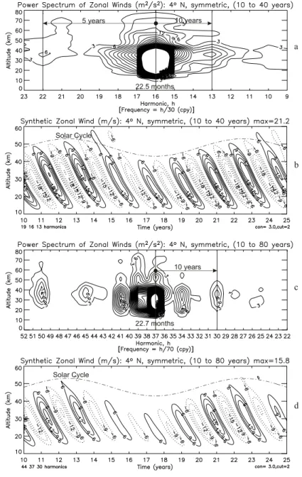
As shown in Fig. 3, the zonal winds for the QBO and SAO near the equator are fairly realistic. The winds at 30 km are almost 20 m/s, and at 50 km the amplitudes for the SAO ex-ceed 30 m/s. For both solutions, with and without SC, the av-erage period of the QBO turns out to be about 22.5 months, which is near the lower end of the observed range.
Mayr et al. (2006) presented results for the computed SC modulation of the QBO from computer runs covering 40 and 60 years. It is shown there that the model can qualitatively reproduce the observations of Salby and Callaghan (2000). In the present paper, we discuss also the numerical results for a computer run of 80 years to demonstrate that the mod-eled SC modulation is robust. However, with increasing time spans, the variability of the QBO becomes more evident and
Fig. 3. Monthly average of computed zonal winds near the equator
at 4◦latitude (Gaussian point). With a period close to 24 months, the Quasi-biennial Oscillation (QBO) has an amplitude of almost 20 m/s at 30 km. Higher-up, the Semi-annual Oscillation (SAO) dominates with amplitudes exceeding 30 m/s.
interferes with the SC signature, which complicates the in-terpretation of the numerical results. This kind of variability could also mask and complicate the observed SC signatures in the real world when more extended data records are ana-lyzed.
In Fig. 4a, we present from Mayr et al. (2006) the power spectrum for the hemispherically symmetric component of the zonal winds at 4◦latitude (Gaussian point) near the equa-tor, taken from the computer run with SC and covering a period from 10 to 40 years (the first 10 years are ignored to allow for spin up). Applying Fourier analysis, the abso-lute amplitudes for the discrete harmonics, h, are recorded as functions of altitude, and contours are drawn to produce the figure. For the short time span of 30 years in this case, the QBO is well defined at harmonic h=16, which repre-sents a period of 30/16 (years)=22.5 months. The spectrum in Fig. 4a also shows separate individual features, and the one at h=13 is of interest in the context of the present study. Displaced from the dominant QBO at h=16 by 3 wave num-bers, this side lobe is the signature of the imposed 10-year SC forcing. A 5-year component is also visible at h=22(16+6). The spectral side lobes are effectively produced by non-linear interactions involving the QBO and the SC forcing. With abbreviated complex notation, the product between QBO, Aexp[i(ωat], and SC, Bexp[i(ωbt], generates the sum and
dif-ference of the frequencies involved, i.e., C1exp[i(ωa+ωb)t]
and C2exp[i(ωa−ωb)t].
We note parenthetically that the displayed spectrum in terms of discrete Fourier harmonics, instead of frequencies or periods, allows the SC signatures to be readily identified. The 10-year side lobe in Fig. 3a at h=13, for example, rep-resents a period of 360 months/13=27.6923 months, which does not tell us, up-front, how it is related to the QBO of
22.5 months at the harmonic h=16. With Fourier harmon-ics, h, in contrast, it is immediately clear that the spectral feature at h=13 – removed from the QBO at h=16 by 3 (the third harmonic of 30 years) – represents the 10-year SC sig-nature of the QBO. Our way of presenting the spectra is per-haps uncommon but proves to be convenient. For the syn-thesis shown in the following Fig. 4b, it is also an advantage to identify the amplitudes with harmonics (displayed at the left bottom of the panel), instead of periods, which are rather meaningless in the present context.
To isolate and reveal the SC modulation of the QBO, we present in Fig. 4b a synthesis of the harmonics at h=16 to-gether with the 10-year side lobe, h=16−3=13, which is identified. We also include the computed signal from the harmonic h=16+3=19, although it is not pronounced in the spectrum for the chosen contour interval. The QBO results in Fig. 4b are presented only for 15 years, which is sufficiently long to reveal the pattern. Since the synthesis describes the 30-year average of the SC modulated QBO, the same pat-tern continues throughout the entire time span from 10 to 40 years. From Fig. 4b it is apparent that the magnitude of the average SC modulation is relatively large, causing the QBO amplitude to increase from about 12 to 21 m/s at 30 km. For comparison we present with dashed line the phase of the im-posed 10-year SC heating, which indicates that the peak of the QBO occurs close to the solar maximum. We emphasize that this correlation with the SC, apparent in the synthesis, is essential for demonstrating the causality of the solar influ-ence; because 10-year spectral side lobes, in principle, could also appear without systematic forcing.
In the lower two panels of Fig. 4, we present the numeri-cal results for the zonal winds near the equator taken from the computer run extended to 80 years. Ignoring again the first 10 years, the 70-year time span is analyzed. Compared to the spectrum shown in Fig. 4a, the QBO signature in Fig. 4c is much more complicated. Instead of a single isolated peak describing an almost monochromatic QBO, the spectrum is broadened to indicate that the period and amplitude vary con-siderably over this longer time span. For the purpose of our study, we shall ignore this variability and take the dominant 22.7-month period at h=37 to represent the average QBO. Corresponding to this QBO, a pronounced 10-year SC side lobe is apparent at h=37−7=30, and a weaker signal is also visible at h=37+7=44. On a statistical basis, it is reasonable to expect that the SC signature would preferentially appear as a modulation of the average and dominant QBO period. To reveal the SC modulation of the QBO period, analogous to Fig. 4b, we present in Fig. 4d a synthesis of the harmon-ics at h=37 together with the 10-year side lobes at h=37±7. From Fig. 4d it is apparent that the magnitude of the average SC modulation is again relatively large, as in Fig. 4b, caus-ing the QBO amplitude to increase from about 6 to 15 m/s at 30 km. The phase of the imposed SC heating also indicates that the peak of the QBO occurs close to the solar maximum. The results presented here thus confirm those reported earlier
Fig. 4. (a) Power spectrum for the hemispherically symmetric component of the zonal winds, presented in terms of discrete Fourier
harmon-ics, h, which are related to the frequency ν=h/y (cpy) in units of cycles per year (y). The time span for the analysis is 30 years, ignoring the first 10 years to account for spin-up. With harmonic h=16, the dominant QBO period is 22.5 months. The side lobe at h=13, removed from the QBO at h=16 by 3 (3rd harmonic of 30 years), thus describes the 10-year SC modulation of the QBO. (Presenting the spectrum in terms of Fourier harmonics allows the SC signatures to be readily identified.) (b) To reveal the SC modulation of the QBO, the dominant QBO harmonic at h=16 is synthesized with the side lobes that describe the 10-year SC signatures, i.e., h=13 (16−3) and 19 (16+3), and the harmonics are given at the lower left bottom of the panel. The contour interval is 2 m/s and the lowest contours are chosen to be 6 m/s to reveal more readily the magnitude of the amplitude modulation. Although the pattern of the QBO modulation is only presented for 15 years, it remains constant and continues to repeat throughout the entire 30-year time span. With dashed line, the phase of the SC forcing is shown for comparison to indicate that the amplitude modulation peaks near the solar maximum. The results are identical to those discussed in Mayr et al. (2006). (c) Analogous to (a) but showing the power spectrum for the model run 10 to 80 years. With the longer time span of 70 years, the spectrum is more complicated and reveals the variability of the QBO. The dominant QBO period is identified at h=37 for a period of 22.7 months. The 10-year SC signature for this period then occurs at h=30 (37−7). (d) Similar to (b), the synthesized winds are presented for the SC modulation of the QBO, involving the harmonics h=37 with 37±7. Although the dominant QBO is weaker compared to (b), the SC modulation is comparable in magnitude, and the phase again is close to that of the imposed SC.
Fig. 5. Similar to Fig. 4 but for the temperature variations of the QBO at 84◦latitude (Gaussian point). (a) As shown, a QBO temperature signature is generated in the troposphere, and the harmonic for the dominant amplitude at h=16 is identical to that for the zonal winds near the equator (Fig. 4a). The side lobes for the 10-year SC occur at h=(16±3), and the 5-year component is visible at h=22 (16+6). (b) The synthesis of the QBO with 10-year SC signatures produces small (<1 K) temperature variations in the troposphere below 10 km.
(Mayr et al., 2006), where time spans of 30 and 50 years were analyzed to describe the SC modulation of the QBO. For windows from 30 to 70 year, in 10-year increments, the synthesized SC modulations of the QBO (not shown) reveal a persistent pattern similar to that evident in Figs. 4b and d. While the maximum amplitude of the QBO, for the dominant period, decreases with increasing time spans, the difference between maximum and minimum of about 10 m/s remains almost constant. The phase of the amplitude modulation rel-ative to the SC forcing also remains the same, demonstrating causality.
Our model results without SC, not presented for brevity, reveal that the dominant QBO periods are not much af-fected by the imposed 10-year modulation of the solar heat-ing. Otherwise, however, the spectral contents differ signifi-cantly. Although there are 10-year spectral signatures gener-ated around the dominant QBO, the synthesized response in each case has no resemblance to that obtained with SC. With the model run covering the 30-year time span, for example, the amplitude modulation is negligible when compared with Fig. 4b. The modulation is relatively large for 70 years, but its phase is almost opposite to that generated in Fig. 4d. In summary, without SC, the synthetic 10-year modulations are comparatively weak or vary erratically. This behavior ob-viously reflects the lack of systematic solar forcing and can
be attributed in part to the variability of the QBO generated internally, which is later discussed.
4.2 Polar QBO temperature variations
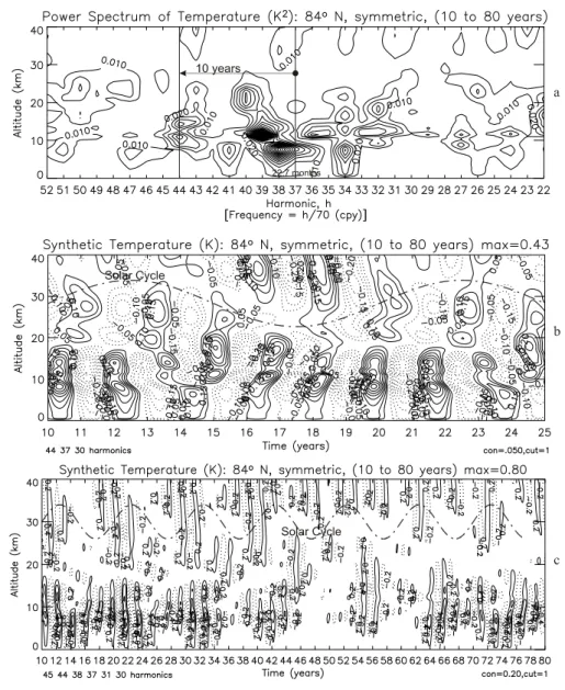
Although the QBO is generated in the zonal circulation of the equatorial region, our model results show that its signa-tures extend to the temperature variations in the troposphere at high latitudes. This is clearly apparent in the numerical results for time spans up to 50 years where the QBO period is more sharply defined. Corresponding to Fig. 4, we present with Fig. 5 for the 30-year window the computed tempera-ture variations near the pole at 84◦latitude (Gaussian point). The results are presented for the altitude range from 40 km down to the Earth’s surface where the temperature perturba-tions are forced to zero with the boundary condiperturba-tions. As is apparent from Fig. 5a, a sharp amplitude maximum occurs at h=16 corresponding to the QBO feature in Fig. 4a that repre-sents a period of 22.5 months. The 10-year SC signatures are pronounced at h=13 and 19 as indicated, and the 5-year com-ponent is also evident at h=22. The synthesized temperature variations in Fig. 5b show that the computed SC modulation of the QBO occurs primarily in the troposphere below 10 km, but it is relatively weak, less than 1 K. The temperature re-sults in the Polar Region for the 50-year time span presented in Mayr et al. (2006) also show that the spectral harmonic for
Fig. 6. (a) Similar to Fig. 5a but for the model run from 10 to 80 years. Assuming that the oscillation originates at equatorial latitudes, the
identified spectral features are consistent with the dominant QBO at h=37 in Fig. 4c. The synthesis (b) then employs the harmonics h=37 and 37±7 to describe the average SC modulation of the QBO. The amplitude maximum in (a) however does not occur at h=37 (for the equator) but at h=38 instead, shifted by one wave number to indicate that the QBO at high latitudes is varying significantly over the time span of 70 years. This variability is evident in the synthesized temperature (c), which employs the harmonics h=37 and 37±7, combined with h=38 and 38±7.
the dominant QBO signature coincides with that of the zonal winds near the equator, and the pattern for the synthesized SC variation is qualitatively similar to that shown in Fig. 5b. For the time span of 70 years, like that of 60 years, the largest temperature amplitudes in the Polar Regions do not occur at the harmonic that defines the dominant QBO period near the equator. This is evident in Fig. 6a (corresponding to Fig. 4c), where we present the temperature power spectrum at 84◦latitude. While the amplitude maximum for the QBO occurs at h=37 near the equator, it appears instead at h=38 near the pole. Displaced by wave number 1, the distortion of
the spectrum signifies that the QBO varies considerably over 70 years. It is reasonable to assume, and consistent with the above-discussed model results for time spans up to 50 years, that the primary temperature signature at high latitudes is de-termined by the dominant period of the QBO near the equator where the oscillation is generated through wave interactions with the zonal winds and where most of its energy is con-centrated. Analogous to Fig. 4d for the equatorial QBO, as identified in Fig. 6a, we present then in Fig. 6b the synthetic temperature variations at polar latitudes that are generated by h=37 and h=37±7. The results show a small SC modulation
of ∼0.5 K in the region around the tropopause, where the largest amplitudes occur relatively close to those shown in Fig. 5b for the 30-year time span. When we examine the synthetic temperature variations covering time spans from 30 to 70 years, the SC effect consistently tends to be largest in the troposphere and lower stratosphere. The phase rela-tionship relative to the SC however is found to be variable, and this apparently reflects the fact that the dynamical pro-cesses involved in transferring the QBO to high latitudes are more complicated than those that generate the primary oscil-lation around the equator. The long-term variability at high latitudes is illustrated in Fig. 6c, where we present the tem-perature variations that are produced from a synthesis of the spectral lines at h=37 and 37±7, as in Fig. 5b, combined with h=38 and 38±7 to account for the 70-year variations. For a period up to almost 50 years, a fairly persistent pattern is evident in the SC modulation, which is in substantial agree-ment with our analysis of the shorter model record. After 50 years, the SC modulation substantially weakens and later re-turns with different phase. This variability of the QBO and its SC modulation could be produced by long-period (e.g., quasi-decadal) oscillations that in turn can be generated by the QBO interacting with the seasonal cycles (Mayr et al., 2003a), and we shall later return to discuss this subject.
5 Solar cycle modulated Equatorial Annual Oscillation (EAO)
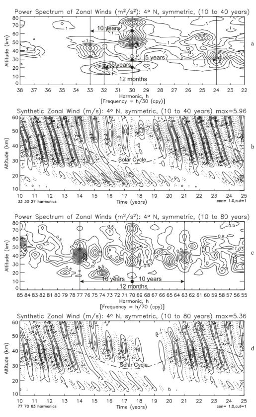
The numerical results presented in the previous section show that the modeled QBO contains a pronounced and persistent SC signature, at least at equatorial latitudes where the os-cillation originates – and the question is what causes the ef-fect. Solar forcing through the seasonal variations must be involved, and the Semi-annual Oscillation (SAO) would ap-pear to be the likely candidate. In their theory for the QBO, Lindzen and Holton (1968) originally invoked the SAO to seed the QBO. The SAO has in common with the QBO that it is confined to low latitudes where it is driven or amplified by waves (e.g., Dunkerton, 1979; Hamilton, 1986). Contrary to expectation, however, a search for SC signatures in the SAO proved the effect to be weak and erratic.
As reported in Mayr et al. (2005), the model generates in-stead a 12-month annual oscillation – which is induced and modulated by the SC and is the pathway and pacemaker for the SC modulation of the QBO. This annual oscillation is hemispherically symmetric, and in the zonal winds it is con-fined to equatorial latitudes like the QBO and SAO. We shall therefore refer to it as Equatorial Annual Oscillation (EAO). Stimulated in part by reviewers of the present paper, Mayr et al. (2007) carried out an analysis of NCEP data, which shows that the observed (assimilated) zonal winds contain an annual oscillation that is also hemispherically symmetric and peaks at the equator.
Adhering to the above format for the analysis of the QBO, Fig. 7a (analogous to Fig. 4a) reproduces the spectrum for the hemispherically symmetric component of the zonal winds at 4◦latitude, describing the discrete Fourier harmonics around the 12-month EAO. The analysis covers again the time span from 10 to 40 years, and the results are identical to those presented in Mayr et al. (2005). The spectrum shows a pro-nounced and isolated feature at the harmonic h=30, which represents the 12-month oscillation. Removed by wave num-ber 3 at h=33 is the 10-year SC signature, and the second harmonic at h=24 is also excited. (An internally generated 15-year oscillation accounts for the side lobe at h=32 and will be discussed later.) In Fig. 7b, we present then a syn-thesis of the spectral features for the SC modulation of the EAO, i.e., h=30 with h=30±3. This shows that the EAO slowly propagates down, with the largest amplitudes occur-ring in the stratosphere at around 40 km. The SC modulation in the region is large, and it is in phase with the solar forcing. It is also in phase with the SC modulation of the QBO, which is evident from a comparison with Fig. 4b. This EAO is ap-parently the pathway and pacemaker for the solar influence on the QBO and thus plays a pivotal role in the SC mecha-nism discussed here. Although the zonal velocities are only about 6 m/s, the large amplitude modulation contributes sig-nificantly to the SC effect in the stratosphere considering the small variations in the solar radiation absorbed there.
The slow downward propagation of the symmetric EAO shown in Fig. 7b, at a rate of about 3 km/month, is charac-teristic of the wave forcing that dominates the dynamics at equatorial latitudes in the stratosphere. This feature is dis-tinctly different from that of the 12-month anti-symmetric annual oscillation (not shown), which reveals virtually no time progression with altitude, and no SC modulation, as shown in Fig. 1c of Mayr et al. (2005). Although the modeled anti-symmetric annual oscillation is much larger in the lower mesosphere, it does not extend into the lower stratosphere like the symmetric component. Without the wave amplifi-cation that is so effective for the EAO, the anti-symmetric oscillation decays rapidly at lower altitudes.
To demonstrate that the SC modulation of the EAO per-sists for many cycles and is robust in the model, we present in Fig. 7c the spectrum for the computer run from 10 to 80 years. In this case, the 12-month oscillation occurs at the harmonic h=70, and the side lobes for the 10-year SC oc-cur at h=63 and 77 (i.e., 70±7). (The spectral side lobes at h=70±5 and h=70±4 are likely the signatures of the above-mentioned 15-year oscillation.) Unlike the spectrum for the QBO, which tends to broaden with increasing time spans, due to the variability of its period, the spectral features defin-ing the 12-month oscillation remain relatively sharp as seen from Fig. 7c. Accordingly, the associated SC signatures are then also well defined. The synthesized zonal winds for the SC modulated EAO are presented in Fig. 7d. As is the case for the shorter 30-year time span (Fig. 7b), a pronounced SC modulation is apparent. The amplitude maximum occurs
Fig. 7. (a) Similar to Fig. 4a but for the (hemispherically) symmetric 12-month annual oscillation covering the time span from 10 to 40
years (also shown in Mayr et al., 2005). For the zonal winds, the oscillation is confined to equatorial latitudes and is therefore referred to as Equatorial Annual Oscillation (EAO). The EAO is modulated by the SC, as the 10-year side lobes indicate that are identified. (b) Synthesis of the spectral features h=33, 30, 27, which describe the SC modulation. Although the magnitude of the EAO is relatively small, its SC modulation is large, and it is in phase with the imposed solar forcing. The SC modulation is also in phase with that of the QBO (Fig. 4b) to indicate that it is the pathway and pacemaker for the solar influence. (c) Similar to (a) but for the time span from 10 to 80 years. (d) The synthesized EAO shows a pattern similar to that in (b) to demonstrate that its SC modulation is a robust feature of the model.
Fig. 8. (a) Like the QBO, the SC modulated symmetric EAO is largely confined to low latitudes (the contour interval is 0.4 m/s). (b)
In contrast to the EAO, the dominant anti-symmetric annual oscillation vanishes at the equator, increases towards mid latitudes, and the SC signature is weak. (c) When the symmetric and anti-symmetric annual oscillations are combined, the resulting SC modulations are pronounced and differ in magnitude and phase in the Northern and Southern Hemispheres (as in b, the contour interval is 2 m/s).
again close to the peak of the solar forcing and is in phase with the SC modulation of the QBO (Fig. 4d). When the synthetic SC modulations of the EAO are examined for time spans from 30 to 50 years, the maximum amplitudes between 30 and 60 km are found to decrease from almost 6 to 3.5 m/s – and we attribute this to the interference from a 15-year os-cillation, generated internally, which is later discussed. The maximum amplitude then increases again to reach values close to 6 m/s for the time spans of 60 and 70 years. Irre-spective of the variable amplitude maximum, we find that the phase relationship relative to the SC remains constant owing to the imposed 10-year SC forcing.
That the EAO of the zonal winds discussed here is con-fined to low latitudes is shown in Fig. 8a, where we present at 30 km a synthesis of the computed SC variations. The
SC modulated EAO peaks at the equator and virtually dis-appears at latitudes above 20◦. In contrast to the EAO, the
regular anti-symmetric annual oscillation, shown in Fig. 8b, vanishes at the equator and increases towards mid latitudes, and its SC modulation is weak. When the two annual os-cillations, symmetric and anti-symmetric, are combined in Fig. 8c, a pronounced SC modulation is introduced owing to the EAO. Depending on the phase of the SC, the symmet-ric EAO reinforces the anti-symmetsymmet-ric annual oscillation in one hemisphere and weakens it in the other. As a result, the amplitude modulation then is larger in the Southern Hemi-sphere where the peak occurs near the SC maximum, while the weaker modulation in the Northern Hemisphere peaks near the SC minimum.
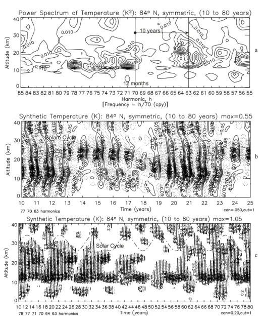
Fig. 9. Similar to Fig. 6 but for the temperature variations at polar latitudes, which are associated with the EAO zonal winds. In (a), the
12-month oscillation is identified at h=70 together with the corresponding SC side lobe, and the synthesis is presented in (b). As in Fig. 6, the amplitude maximum in (a) occurs at h=71 instead of 70, shifted by one wave number to indicate the 70-year variability. The synthesis in
(c) then describes the SC modulation of the symmetric annual oscillation over the 70-year time span.
As is the case for the SC modulation of the QBO, the EAO produces temperature variations in the Polar Regions. Anal-ogous to Fig. 6a for the QBO results covering the time span from 10 to 80 years, we present in Fig. 9a the spectrum for the symmetric annual component at 84◦latitude. Similar to the situation for the QBO, the harmonic with the largest am-plitude at h=71 is displaced by one wave number to indicate significant variability over 70 years. For the synthetic tem-perature variations shown in Fig. 9b, we ignore this shift in the spectrum and take instead the amplitudes of the spec-tral lines that define the SC modulated EAO at h=70 and 70±7, which dominate near the equator (Fig. 7c). Except for the magnitude, the resulting pattern of the SC modulation is similar to that for the 30-year time span shown in Mayr et
al. (2005). When the spectral features of the EAO temper-ature signtemper-ature, with its 10-year side lobes, are synthesized for time spans from 30 to 70 years (not shown) the ampli-tudes decrease and the phase relationship relative to the SC varies but not significantly. In all cases, the largest ampli-tudes below 15 km occur near the SC maximum. The high-latitude pattern in Fig. 9b indicates that the oscillation ap-pears to propagate down from the stratosphere to produce in the temperature a small SC modulation of about 0.5 K near the tropopause. Analogous to Fig. 6c for the SC signature in the QBO at polar latitudes, we present in Figure 9c the cor-responding synthesis for the symmetric annual oscillation, which characterizes the long-term variations. In this case, the amplitudes are synthesized for the spectral lines h=70
Fig. 10. Similar to Fig. 8 but for the temperature variations at 15 km, which are associated with the symmetric EAO zonal winds. In
contrast to the zonal wind oscillations (Fig. 8a), which are confined to equatorial latitudes due to wave mean flow interactions, the associated temperature variations extend to high latitudes.
and 70±7, combined with h=71 and 71±7 to account for the 70-year variability. The general pattern of the long-term variation is similar to that shown in Fig. 6c for the QBO. For the initial few solar cycles, a persistent pattern is evident in the SC modulation, which is consistent with the larger ampli-tudes in the above discussed results from the shorter model records. The SC modulation significantly weakens after 40 years, then increases again during the last two cycles. Com-pared with the variability in the SC modulation of the QBO at high latitudes (Fig. 6c), however, the corresponding pattern in the symmetric annual oscillation is more stable, which is understandable considering that the period of 12 months it-self is constant.
To reveal the global character of the symmetric annual os-cillation, we present in Fig. 10 the latitudinal variations of the temperature variations at 15 km, which are obtained from a synthesis of the harmonics h=70 and 70±7, as applied in Figs. 9b to describe the average SC signature. In contrast to the zonal wind pattern shown in Fig. 8a, the temperature variations extend to high latitudes and are larger in the Polar Region than at the equator. The phase progression indicates that the oscillation propagates from the equator towards the poles, which is consistent with our assertion that it originates in the EAO zonal winds at low latitudes where most of the energy resides.
Apart from its pivotal role as pacemaker for the SC mod-ulation of the QBO, the EAO is also of interest in its own right. Like the QBO and SAO, the EAO is driven by wave mean flow interactions at equatorial latitudes, and such a dy-namical phenomenon has not been discussed in the litera-ture before. In partial support of our model results, however, some observational evidence for the EAO has come from an analysis of NCEP data (Mayr et al., 2007) mentioned earlier. In that paper it is shown that a hemispherically symmetric annual oscillation is observed in the mean zonal winds of the lower stratosphere. This oscillation is modulated by a pe-riod of 5 years, which is apparently generated internally by
a QBO of 30 months as predicted (Mayr et al., 2000). The inferred 5-year modulation of the zonal wind oscillation is confined to equatorial latitudes. In the temperature data, the 5-year modulation is also evident, but it extends to the Polar Regions, which is in qualitative agreement with our model results.
6 Solar cycle mechanisms
6.1 Seasonal variations
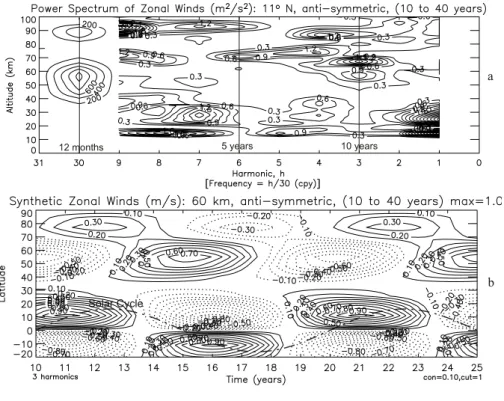
To shed light on the process that generates the EAO in the model, we present in Fig. 11a the spectrum for the anti-symmetric component of the zonal winds at 11◦latitude ob-tained from an analysis of the time span from 10 to 40 years. (This component vanishes at the equator.) Two regimes are shown in the spectrum. One covers the harmonics 0<h<9, and it reveals the spectral features that describe the long-term variations with periods as short as 5 years. The other one cov-ers only the harmonics around h=30 to describe the dominant anti-symmetric 12-month oscillation. In Fig. 11a, a distinct 10-year SC signature is apparent at altitudes around 60 km in the mesosphere, and the weaker 5-year component is also evident. With Fig. 11b, we present then the synthesis for h=3 at 60 km, which describes the latitude dependence of the 10-year anti-symmetric SC signature that is generated in the model. This signature of the direct SC forcing is fairly robust in the model, as shown in Figs. 11c where we show the re-sults for the computer run extended to 80 years. The 10-year spectral feature again is concentrated at around 60 km alti-tude, and the synthesized zonal winds in Fig. 11d at low to mid latitudes are in reasonable agreement with Fig. 11b for the shorter time span.
With a constant SC period of 10 years, the maximum of the cycle occurs in the model during northern summer solstice. This synchronizes the solar variability and the seasonal (an-nual) variations so that the SC signatures in Figs. 11b and
Fig. 11. (a) Spectrum of the anti-symmetric zonal wind component for the time span from 10 to 40 years, covering the harmonic range
0<h<9 to reveal the 5- and 10-year SC signatures. At h=3, a relatively sharp but weak feature appears at altitudes around 60 km in the mesosphere, which reflects the small SC heating applied in the model. Also shown is the spectrum around the dominant, and much larger, anti-symmetric 12-month oscillation at h=30 (note the different contour intervals). (b) Synthesis of the anti-symmetric 10-year SC component at h=3 shows small wind velocities at 60 km varying with latitude. These winds interact apparently in a non-linear way with the strong anti-symmetric 12-month oscillation and thus produce the SC modulated symmetric EAO shown in Fig. 7. (c) Similar to (a) but for the model run from 10 to 80 years, showing again the sharp SC signature at around 60 km. (d) The synthesized winds reveal a pattern very similar to that in (b), which reflects the persistent SC forcing applied in the model.
d are anti-symmetric like the annual oscillation. The small zonal wind amplitudes are consistent with the weak SC mod-ulation of the heat source applied in the model.
Non-linear interaction between this weak 10-year oscilla-tion and the strong anti-symmetric annual oscillaoscilla-tion (h=30, Fig. 11a; h=70, Fig. 11c) then generates presumably the SC modulated symmetric EAO discussed in Figs. 7 through 10. 6.2 Amplification by wave-mean-flow interaction
Our numerical results indicate that the dynamical conditions at low latitudes, and the wave forcing in particular, are of critical importance for the large SC modulation of the QBO generated in the model. Since the equatorial oscillations are driven primarily by parameterized small-scale gravity waves (GW), the model was run again for diagnostic purposes to record the associated momentum source (Fig. 1b). The com-pleted computer run covers 60 years, and for comparison with the QBO and EAO results (Figs. 4a, b; 7a, b) we present the momentum source for the time span from 10 to 40 years. (The results are virtually identical for the longer model run from 10 to 60 years.)
In the model, the non-linear GW momentum source (MS) is computed in physical space along with all the other non-linearities. Unlike the winds and temperature variations that are supplied for m=0 as part of the solution, the MS record covers all the zonal wave numbers (m=0 to 4), and it is there-fore much larger. To reduce the model output, the MS has been recorded in 5 km altitude intervals instead of 0.5 km (the vertical model resolution). With reduced vertical resolution, the displayed results for the MS therefore appear ragged.
Since the MS for the GWs varies exponentially with height, its height dependence is effectively eliminated for display. This is accomplished by normalizing at each altitude the amplitudes (for the spectrum) and the synthesized max-imum values (positive or negative) to a dimensionless value of 10. The normalization preserves the relative SC variations with time, which are of interest for the present purpose.
With the format used to describe the SC modulations of the QBO and EAO, we present in Fig. 12 the spectra and synthesized variations of the normalized MS. As expected, the amplitude maximum for the QBO occurs at h=16, cor-responding to the period of 22.5 months for the zonal winds in Fig. 4a. This sharp spectral feature dominates at altitudes between 10 and 50 km, where the GWs generate the QBO in the stratosphere. Weaker spectral features are also evident at h=13 and 19, which are removed by 3 wave numbers from h=16 to describe the 10-year SC signatures. In Fig. 12b, we then present for the MS the synthesis of the spectral features at h=13, 16 and 19. This shows that the MS varies at 40 km by almost a factor of 2, and it varies in phase with the SC forcing. Through the positive non-linear feedback in the MS, evident from Fig. 1b, the SC influence on the QBO is in effect amplified. Since the GW source in the troposphere is taken to be time independent, the large SC modulation of the MS
in Fig. 12b is solely produced by this non-linearity – which we believe is not just a property of the GW interaction but is characteristic of the wave forcing in general, planetary waves included, that is required to generate the QBO.
Analogous to Fig. 12a, we present with Fig. 12c the nor-malized MS, which is involved in generating the zonal winds in Fig. 7 for the symmetric annual oscillation or Equatorial Annual Oscillation (EAO). Although ragged due to the 5-km resolution of the recorded MS, the spectrum nevertheless re-veals the salient features that describe the SC modulation of the EAO. The 12-month oscillation is apparent at h=30, and the side lobes at h=27, and at 33 in particular, describe the 10-year SC variation. As in Fig. 7a, there is also the feature at h=32, which is the signature of a 15-year oscillation later discussed. A synthesis of the harmonics h=30 with 30±3 is then presented in Fig. 12d, and it shows that the MS for the symmetric EAO varies at 40 km by as much as a factor of 4 between the minimum and maximum of the imposed SC forcing. The modulation of the MS is in phase with the SC and with that of the zonal winds for the symmetric EAO (Fig. 7b).
Considering the unique dynamical properties that control the symmetric zonal wind oscillations at equatorial latitudes, the results presented in Fig. 12 are reasonably well under-stood. The waves propagating up encounter vertical zonal wind shears where they deposit momentum and thus increase the shears. At equatorial latitudes, as pointed out by Lindzen and Holton (1968), the wave source is very effective because it is mainly dissipated by viscosity, unlike the region outside the tropics where the meridional circulation also comes into play to redistribute the momentum. Due to the non-linear positive feedback in the wave momentum source, the SC modulations of the QBO and EAO are therefore amplified.
The above-discussed mechanisms lead to the conclusion that several interlocking stages or processes are involved in generating the SC modulation of the QBO in our model. (1) The variable but systematic solar forcing produces in the mesosphere a 10-year SC oscillation (Fig. 11b), which is hemispherically anti-symmetric (opposite phase in the two hemispheres). (2) This SC signature interacts with the domi-nant anti-symmetric 12-month oscillation (shown in Fig. 11a at h=30) to produce the symmetric SC modulated EAO. (3) The EAO thus generated is amplified by the upward propa-gating waves (Fig. 12d) and propagates down to lower alti-tudes like the QBO (Fig. 7b). (4) Due to the positive feed-back in the wave momentum source, the stratospheric EAO becomes apparently the seed and pacemaker for the SC mod-ulation of the QBO (see Figs. 4b and 7b for comparison). (5) Like the EAO, the QBO is then amplified by tapping the mo-mentum from the upward propagating waves (Fig. 12b). The aggregate effect is that the QBO in the lower stratosphere is produced with a relatively large SC modulation, which is in qualitative agreement with the observations (Salby and Callaghan, 2000).
Fig. 12. Gravity wave (GW) momentum source (MS) for the time span from 10 to 40 years, based on a wave source in the troposphere that is
time independent. To eliminate from view the exponential variation of the MS, a normalization is applied that preserves the time-dependent SC modulation of interest. Although the vertical resolution of the model is about 0.5 km, the MS is recorded with 5 km height increments to reduce the model output. The results therefore appear ragged. (a) With the maximum MS normalized to the value 10, and the lowest contour at 3, the spectrum peaks at h=16 (22.5 months), consistent with the zonal wind oscillations in Fig. 4a. The side lobes for the 10-year SC modulation are also evident. (b) The synthesis for the spectral features at h=13, 16 and 19 shows a pronounced amplitude modulation, which is essentially in phase with the imposed SC (dashed line), and with the zonal winds in Fig. 4b. With contour intervals of 2, the maximum amplitudes are close to 10 (as defined), while the minimum values are only around 5. This demonstrates that the GW source significantly amplifies the SC modulation of the QBO, which represents a new mechanism for the solar influence on the lower atmosphere. (c) Similar to (a) but for the normalized MS that drives the symmetric annual oscillation or EAO shown in Fig. 7. At h=30, the 12-month periodicity is evident, and the spectral features at h=27, and at 33 in particular, describe the 10-year SC signatures. As in Fig. 7a, the 15-year signature is also pronounced. (d) The synthesis of the harmonics h=33, 30 and 27 describes the SC modulation of the MS for the EAO, which is in phase with the imposed solar forcing and with the zonal winds in Fig. 7b.
7 Internally generated long-term variations
In light of the SC driven quasi-decadal oscillations discussed here, it is of interest that long-term variations can also be gen-erated in the atmosphere internally. It was shown in a study with the 2-D version of the NSM that the QBO, depending on its periodicity, can generate long period oscillations through interaction with the seasonal cycles (Mayr et al., 2003a). As illustrated in Fig. 1 of that paper, the proposed mechanism involves GW node filtering, and it is briefly discussed here.
The GWs propagating up through the nodes of the QBO, with period τQ, are less attenuated and thus carry its
im-print. When the QBO nodes, with enhanced GW flux, are aligned with the opposite phase of either the symmetric 6-month SAO or the dominant anti-symmetric 12-6-month oscil-lation in the zonal winds, the waves amplify the velocities to produce half of the beat period, τB, which defines the
long-term oscillation. In numerical long-terms this requires that the condition
τB =2N × τQ= [2n + 1] × (12, 6), in months (2)
is satisfied, where N and n are integers, and the annual or semi-annual components of the seasonal variations have pe-riods of 12 or 6 months, respectively. This mechanism was demonstrated with numerical results from the 2-D model, which produced beat periods of 5 and 9 years for QBO pe-riods of 30 and 27 months, respectively (Mayr et al., 2000, 2003a). As mentioned earlier, the association between the 30-month QBO and the 5-year oscillation is evident in NCEP data (Mayr et al., 2007). This QBO interacts with the 12-month oscillation to generate an anti-symmetric 5-year beat period, which is satisfied with N =1 and n=2 applied in Eq. (2).
As predicted (Mayr et al., 2003a), the QBO of 22.5 months in the present model would interact through wave filtering with the dominant annual oscillation to generate an anti-symmetric oscillation of 15 years (N =4, n=7 for Eq. 2). The non-linear interaction between this oscillation and the dom-inant 12-month oscillation then generates the 15-year side lobes evident in Figs. 7a and 12c, which appear also in the solution without SC forcing.
Although our model scenario with QBO period near 22 months and 15-year beat period is mainly of academic in-terest, considering that the observed QBO is closer to 28 months, our results may serve to illustrate how an inter-nally generated long-term oscillation can interfere with the SC signature. Some evidence of this interference is evident in the SC modulation of the EAO, which in turn should affect also the QBO. For the 30- and 60-year time spans analyzed, the computed SC modulations of the EAO are considerably larger than those derived for the intervening windows of 40 and 50 years where the 15-year oscillation is not resolved. In these latter cases, the cross talk from the 15-year oscilla-tion apparently comes into play to cause interference. In the
present model, this kind of interference could be responsi-ble, at least in part, for the variability of the SC signatures in the QBO and EAO temperature variations at polar latitudes, which are evident respectively in Figs. 6 and 9.
8 Summary, conclusion, and critique
The impetus for the presented study has been the paper by Salby and Callaghan (2000), who analyzed more than 40 years of zonal wind measurements at low latitudes to show that the QBO amplitude exhibits a relatively large SC modu-lation. The model discussed here reproduces qualitatively the observed variations in the lower stratosphere, and initial re-sults were reported elsewhere (Mayr et al., 2005, 2006). This full-length paper presents a more comprehensive description of the model, documents more fully the numerical results, and provides a quantitative understanding of the mechanisms that generate the large SC modulation of the QBO.
The numerical results presented cover a long time span of 70 years and thus provide some confidence that the modeled SC effect is robust. When the synthesized SC modulations of the QBO are examined for time spans from 30 to 70 years, in 10-year increments, the maximum amplitude decreases, but the magnitude of the modulation is almost constant at about 10 m/s at 30 km, evident in Figs. 4b and d. Still more im-portant, the phase of the QBO modulation relative to that of the SC remains essentially constant for the entire time span of the model simulation. That the SC is the cause for the QBO modulation in the model is thus reasonably well estab-lished. For model runs without SC (not shown), in contrast, the corresponding synthetic zonal wind variations reveal pat-terns with weak or erratic amplitude modulations, which re-flect the lack of systematic SC forcing.
The question is what causes the effect, and our numerical results show that a SC modulated annual oscillation acts as pathway and pacemaker for the solar influence on the QBO. This annual oscillation is anomalous in that it is hemispheri-cally symmetric. In the zonal winds, it is confined to equato-rial latitudes and is therefore referred to as Equatoequato-rial Annual Oscillation (EAO). The amplitude of the EAO is relatively small, but its SC modulation is large and is in phase with the solar forcing at least up to 70 years (Fig. 7).
Our analysis shows that the following interlocking pro-cesses are involved in generating the SC modulations of the QBO and EAO.
(1) The variable but systematic solar forcing produces in the zonal winds a 10-year SC component at around 60 km (mesosphere), shown in Figs. 11b, d for the 30- and 70-year time spans, which is hemispherically anti-symmetric (with opposite phase in the two hemispheres). Commensurate with the weak SC heat source applied in the model, the velocities are small (∼1 m/s).
(2) Non-linear interaction between this anti-symmetric SC component and the strong anti-symmetric annual oscillation
(in Figs. 11a, c at h=30, 70) produces the SC modulation that characterizes the symmetric EAO in Fig. 7.
(3) Through non-linear feedback, the EAO is amplified by wave-mean-flow interaction (Fig. 12d), and under that influ-ence the flow oscillation propagates down to lower altitudes like the QBO.
(4) The modulated EAO then acts as pacemaker for the SC modulation of the QBO, as seen from Figs. 4b, d compared with Figs. 7b, d, respectively.
(5) Like the EAO, the SC modulated QBO is then ampli-fied by the GWs as shown in Fig. 12b. Ampliampli-fied by wave mean flow interaction, the QBO thus becomes the conduit that transfers to lower altitudes the influence from the SC variations in the UV absorbed in the mesosphere.
The processes involved in generating the SC modulation of the QBO in our model have in common that they characterize the unique dynamical properties of the equatorial region in the middle atmosphere. We recall what these properties are:
(a) With the horizontal Coriolis force vanishing at the equator, absent dissipation by the meridional circulation, the wave forcing is very efficient there because it is only dissi-pated by viscosity (Lindzen and Holton, 1968). The QBO and EAO of the zonal winds therefore tend to peak at the equator.
(b) Related to this property, the eddy viscosity (generated by wave dissipation) decreases at lower altitudes to produce time constants on the order of years, which partially de-termines the QBO period and favors the generation of SC-related long-term variations.
(c) While QBO-like oscillations can be generated in prin-ciple without time dependent forcing, numerical experiments show that external sources affect significantly the amplitude and period of the QBO (Mayr et al., 1998). Not being tied to a particular period, this property we believe makes the QBO pliable so that it can be influenced and guided by the SC mod-ulated EAO that acts as pacemaker.
Generated in part by the meridional circulation, and plan-etary waves presumably, the QBO signature extends to high latitudes to produce tropospheric temperature variations in the Polar Regions. This is clearly evident in the spectrum for the time span of 30-years (Fig. 5), where the period of the equatorial QBO in the zonal winds is sharply defined (Fig. 4a). For the longer time spans of 60 and 70 years, the variability of the QBO period however becomes evident in the broadening of the spectrum (e.g., Fig. 4c), and the po-lar signal in the temperature (Fig. 6) is then less coherent. A contributing factor presumably is the added complexity of the dynamical processes that are involved in redistributing the energy from the equator towards the Polar Regions. As reviewed in the introduction, the equatorial route of the solar influence on the Polar Regions, through the QBO, has been discussed in several papers based on observations and mod-eling studies (e.g., Labitzke, 1982, 1987; Labitzke and van Loon, 1988, 1992; Dunkerton and Baldwin, 1992; Baldwin and Dunkerton, 1998; Matthes et al., 2004; Palmer and Gray,
2005; Pascoe et al., 2005). In the present paper, the polar connection to the QBO is primarily tied to the large SC mod-ulation of the equatorial zonal winds, which is generated in our model and is in qualitative agreement with the observa-tions (Salby and Callaghan, 2000).
Although the EAO is concentrated mainly in the region around the equator, its energy is redistributed by the merid-ional circulation and planetary waves to be partially focused onto the Polar Regions. The signature of the EAO, like that of the QBO, thus appears at high latitudes where the SC produces measurable variations in the temperature near the tropopause. In the model, the SC modulated tempera-ture perturbations seem to propagate down from the upper stratosphere and thus may be involved in generating the Arc-tic Oscillation, which represents a mode of variability that is sensitive to SC influence (e.g., Kodera, 1995; Thompson and Wallace, 1998; Baldwin and Dunkerton, 1999; Ruzmaikin and Feynman, 2002).
Our model however is not entirely realistic. The QBO pe-riod of about 22 months is near the lower end of the observed range. With zonal winds close to 10 m/s at 15 km (Fig. 3), the QBO extends to lower altitudes than observed (e.g., Pascoe et al., 2005). Although the model generates planetary waves through the baroclinic instability near the tropopause, it does not account for the waves produced by topography and trop-ical convection that are resolved in GCMs (e.g., Giorgetta et al., 2001). And the NSM does not account for the feedback involving ozone for example, which contributes to the SC modulation of the QBO (Cordero and Nathan, 2005). With the SC period in the present study fixed at exactly 10 years, the maximum of the cycle occurs during northern summer solstice, which synchronizes the solar variability with the an-nual cycle. Since the SC is variable in the real world, the present model thus describes only one particular scenario or mode of SC forcing.
Notwithstanding the limitations of our model, it offers a SC mechanism to explain the observations by Salby and Callaghan (2000). The model describes a new dynamical pathway for the solar influence on the stratosphere, and our analysis results provide an understanding of the processes in-volved. In the mechanism discussed, the variable solar forc-ing in the mesosphere generates through the seasonal cycle a SC modulated Equatorial Annual Oscillation (EAO), which propagates down into the lower atmosphere under the influ-ence of, and amplified by, wave forcing. Through the EAO as pacemaker, the solar influence is transferred to the QBO to generate the SC modulation, which is then amplified by the wave interaction. Like steering an ocean liner, the energy re-quired to induce the SC modulation at higher altitudes in the mesosphere is relatively small when compared with the en-ergy the waves provide to amplify the flow oscillations in the lower stratosphere. In this process, a SC modulation of the QBO period could prove to be very effective, as our earlier 2-D study indicated (Mayr et al., 2003b).