Climate forcing and air quality change due to regional emissions reductions by economic sector

(1)

HAL Id: hal-00304259

https://hal.archives-ouvertes.fr/hal-00304259

Submitted on 12 Jun 2008

HAL is a multi-disciplinary open access

archive for the deposit and dissemination of sci-entific research documents, whether they are pub-lished or not. The documents may come from teaching and research institutions in France or abroad, or from public or private research centers.

L’archive ouverte pluridisciplinaire HAL, est destinée au dépôt et à la diffusion de documents scientifiques de niveau recherche, publiés ou non, émanant des établissements d’enseignement et de recherche français ou étrangers, des laboratoires publics ou privés.

Climate forcing and air quality change due to regional

emissions reductions by economic sector

D. Shindell, J.-F. Lamarque, N. Unger, D. Koch, G. Faluveg, S. Bauer, H.

Teich

To cite this version:

D. Shindell, J.-F. Lamarque, N. Unger, D. Koch, G. Faluveg, et al.. Climate forcing and air quality change due to regional emissions reductions by economic sector. Atmospheric Chemistry and Physics Discussions, European Geosciences Union, 2008, 8 (3), pp.11609-11642. �hal-00304259�

(2)

ACPD

8, 11609–11642, 2008

Climate and air quality by emission

region and sector D. Shindell et al. Title Page Abstract Introduction Conclusions References Tables Figures ◭ ◮ ◭ ◮ Back Close

Full Screen / Esc

Printer-friendly Version

Interactive Discussion Atmos. Chem. Phys. Discuss., 8, 11609–11642, 2008

www.atmos-chem-phys-discuss.net/8/11609/2008/ © Author(s) 2008. This work is distributed under the Creative Commons Attribution 3.0 License.

Atmospheric Chemistry and Physics Discussions

Climate forcing and air quality change

due to regional emissions reductions by

economic sector

D. Shindell1, J.-F. Lamarque2, N. Unger1, D. Koch1, G. Faluveg1, S. Bauer1, and H. Teich1

1

NASA Goddard Institute for Space Studies, New York, NY, USA 2

National Center for Atmospheric Research, Boulder, CO, USA

Received: 16 May 2008 – Accepted: 25 May 2008 – Published: 12 June 2008 Correspondence to: D. Shindell ([email protected])

(3)

ACPD

8, 11609–11642, 2008

Full Screen / Esc

Interactive Discussion

Abstract

We examine the air quality (AQ) and radiative forcing (RF) response to emissions re-ductions by economic sector for North America and developing Asia in the CAM and GISS composition/climate models. Decreases in annual average surface particulate are relatively robust, with intermodel variations in magnitude typically <30% and very

5

similar spatial structure. Surface ozone responses are small and highly model depen-dent. The largest net RF results from reductions in emissions from the North America industrial/power and developing Asia domestic fuel burning sectors. Sulfate reductions dominate the first case, for which intermodel variations in the sulfate (or total) aerosol optical depth (AOD) responses are ∼30% and the modeled spatial patterns of the AOD

10

reductions are highly correlated (R=0.9). Decreases in BC dominate the developing Asia domestic fuel burning case, and show substantially greater model-to-model dif-ferences. Intermodel variations in tropospheric ozone burdens are also large, though aerosol changes dominate those cases with substantial net climate forcing. The results indicate that across-the-board emissions reductions in domestic fuel burning in

devel-15

oping Asia and in surface transportation in North America are likely to offer the greatest potential for substantial, simultaneous improvement in local air quality and near-term mitigation of global climate change via short-lived species. Conversely, reductions in industrial/power emissions have the potential to accelerate near-term warming, though they would improve AQ and have a long-term cooling effect on climate. These broad

20

conclusions appear robust to intermodel differences.

1 Introduction

Changes in AQ and climate typically occur on different temporal and spatial scales. As climate change is by definition a long-term phenomenon, climate policy typically focuses on well-mixed greenhouse gases, as these have strong radiative forcing and

25

(4)

con-ACPD

8, 11609–11642, 2008

Full Screen / Esc

Interactive Discussion trast, is usually concerned with short-lived pollutants (residence times of months or

less) which do not currently play as prominent a role in climate policy. The two is-sues are linked in several ways, however. Tropospheric ozone and aerosols, among the primary short-lived pollutants regulated for AQ purposes, influence global climate change, and conversely are affected by the impact of climate change on factors such as

5

temperature and humidity. Though emissions of long-lived greenhouse gases, espe-cially carbon dioxide, are the main driver of projected future climate change, AQ-related emissions have the potential to substantially affect 21st Century climate as well (Shin-dell et al., 2008). In addition, AQ-related emissions reductions may lead to substantial economic and health benefits (West et al., 2006; West et al., 2007).

10

AQ regulations are typically made without consideration of their effect on climate. Different regulatory choices potentially affect climate in opposite ways, however, as some AQ-related emissions lead to warming while others lead to cooling. Precipitation may also be either enhanced or suppressed by emissions changes resulting from AQ policy. Hence a carefully designed regulatory approach for short-lived pollutants could

15

both mitigate some of the effects of global warming and improve AQ, while a poorly designed approach could improve AQ but accelerate warming.

To aid in formulation of policies to address both AQ and climate change, we per-formed a series of simulations examining the impact of specific emission sectors on ra-diatively active short-lived species using composition and climate models from the

God-20

dard Institute for Space Studies (GISS) and the Community Atmosphere Model (CAM) model, developed in collaboration with the National Center for Atmospheric Research (NCAR). In addition to calculating RF from short-lived species (in the GISS model), we also estimate the RF from long-lived species for comparison. These species were not simulated by the composition models, so their forcing estimates were instead based

25

on the carbon dioxide (CO₂) and methane (CH₄) emissions from each sector. We concentrate here on the near-term forcing over the next two decades from potential present-day emissions perturbations. This timescale is chosen to be long enough that the climate system would have sufficient time to respond to a substantial portion of

(5)

ACPD

8, 11609–11642, 2008

Full Screen / Esc

Interactive Discussion the forcing from short-lived species, which occurs virtually right away following

emis-sions changes, but not to be so long that AQ-related emisemis-sions would likely diverge enormously from their current levels (the influence of the choice of time horizon is dis-cussed further in Sect. 5).

These experiments were done in support of the US Climate Change Science

Pro-5

gram (CCSP) Synthesis and Assessment Product 3.2: “Climate Projections Based on Emission Scenarios for Long-lived and Short-lived Radiatively Active Gases and Aerosols”. They were designed to examine the climate forcing due to short-lived species in a policy-relevant way by isolating the influence of economic activities subject to regulation and/or reduction in usage (e.g. by improved efficiency). We look at 30%

10

reductions in total emissions from domestic fuel usage (residential and commercial fossil and biofuel burning), surface transportation, and from a combined industry and power generation sector. These three are the main anthropogenic sources for emis-sion of short-lived species and their precursors. Note that the combined industry/power sector can be largely separated into its two components for aerosols, as sulfur

emis-15

sions are largely from power generation while carbonaceous aerosol emissions are mostly from industrial processes (use of the combined sector saves computational re-sources). Since we consider across-the-board reductions in emissions from a given sector, our results are useful for assessing the potential impacts of reductions in total power/fuel usage rather than changes in the mix of power generation/transportation

20

types or in emissions control technologies targeted at specific pollutants. However, we examine both the net forcing from each sector and the contribution from individ-ual species, so that both the sectors and individindivid-ual pollutants within sectors that are the most attractive climate mitigation targets can be determined. The responses to separate emissions perturbations in both North America (60–130 W, 25–60 N) and

de-25

veloping Asia (60–130 E, 0–50 N) are studied. These two regions were chosen based on their being the focus of CCSP interest and being the largest current emitter of many pollutants, respectively.

(6)

ACPD

8, 11609–11642, 2008

Full Screen / Esc

2 Composition and climate models

The components of the GISS model for Physical Understanding of Composition-Climate INteractions and Impacts (G-PUCCINI) version used here include photochem-istry from the surface to the mesosphere (Shindell et al., 2006), and sulfate, carbona-ceous, sea salt, nitrate, and mineral dust aerosols (Koch et al., 2007; Bauer et al., 2006;

5

Miller et al., 2006). Dust and sea-salt are segregated into size bins, nitrate and sulfate aerosols have fine and coarse modes, while only total mass is simulated for carbona-ceous aerosols. The components interact with one another, with linkages including oxidants affecting sulfate, gas-phase nitrogen species affecting nitrate, sulfate affecting nitrogen heterogeneous chemistry, thermodynamic ammonium nitrate formation

be-10

ing affected by sulfate, sea salt and mineral dust (Metzger et al., 2006), and sulfate and nitrate being absorbed onto mineral dust surfaces (Bauer et al., 2006; Bauer et al., 2007). As in our prior CCSP simulations (Shindell et al., 2007), the enhanced con-vective scavenging of aerosols in (Koch et al., 2007) was not included, leading to a higher burden of these species relative to that study but values still roughly consistent

15

with observations. The simulations described here were run using a 4 by 5 degree hor-izontal resolution version of the ModelE climate model with 23-layers extending from the surface to ∼0.01 hPa (Schmidt et al., 2006).

Simulations were also performed using the Community Atmosphere Model CAM3 (Collins et al., 2006) coupled to the Model for Ozone and Related Tracers (MOZART)

20

chemistry (Horowitz et al., 2003). MOZART tropospheric chemistry is an extension of the mechanism presented in (Horowitz et al., 2003); changes include an updated terpene oxidation scheme and a better treatment of anthropogenic and natural non-methane hydrocarbons (NMHCs) treated up to isoprene, toluene and monoterpenes. Aerosols have been extended from the work by (Lamarque et al., 2005) to include

25

actively simulated sea-salt and dust aerosols (each segregated into 4 bin sizes, from fine mode to coarse mode) and a representation of ammonium nitrate that is depen-dent on sulfate following the parameterization of gas/aerosol partitioning by (Metzger

(7)

ACPD

8, 11609–11642, 2008

Full Screen / Esc

Interactive Discussion et al., 2002). Interactions are similar to those in the GISS model, with the

excep-tion that there is no uptake of sulfate and nitrate onto mineral dust. CAM includes secondary organic aerosols, however, which GISS does not, and these are linked to the gas-phase chemistry through the oxidation of atmospheric NMHCs as in (Chung and Seinfeld, 2002). Only the bulk mass is calculated for aerosols other than

sea-5

salt and dust, and all aerosols are radiatively active. The horizontal resolution is 2 by 2.5 degrees, with 26 levels from the surface to ∼4 hPa.

Present-day simulations of trace gases and aerosols in both models agree fairly well with observations over North America for all species as in the model references given previously, while sulfate, BC, OC and CO are all biased low over developing Asia.

10

Such biases are common among models, and have been linked to underestimates of developing Asian emissions in current inventories (e.g. Arellano et al., 2004; P ´etron et al., 2004; Bergamaschi et al., 2000). Ratios of positive and negative forcing agents, e.g. BC/OC or SO₄/BC, are fairly reasonable in both regions, however. Neither model included indirect aerosol effects or radiative forcing from changes in black carbon

de-15

position onto snow and ice surfaces.

3 Experimental setup

Six simulations were performed, each reducing present-day emissions by 30% in one sector for one region. By using present-day emissions, the results are not tied to any particular future scenario. We use IIASA 2000 sectoral emissions (Table 1), based

20

on the 1995 EDGAR3.2 inventory extrapolated to 2000 using national and sector eco-nomic development data (Dentener et al., 2005). The exception is biomass burning emissions, which are averages over 1997–2002 from (Van der Werf et al., 2003) with emission factors from (Andreae and Merlet, 2001) for aerosols. The CAM model did not perform the transportation sector simulations.

25

All simulations kept long-lived greenhouse gases fixed at present day values as these were (generally) not part of the composition models that were used here, which instead

(8)

ACPD

8, 11609–11642, 2008

Full Screen / Esc

Interactive Discussion focused on shorter-lived pollutants. Changes in CO₂and CH₄in response to changes

in anthropogenic emissions of those gases are relatively straightforward to estimate to first-order, and do not require full 3-D chemical-transport models (though such estimate do not include all relevant feedbacks, such as the response of the carbon cycle to climate change). RF from changes in emissions of long-lived species based on such

5

estimates is discussed in Sect. 5. Our primary goal, however, is to use the composition-climate models to calculate the RF from all the short-lived species and hence to identify the relative contributions of the sectors and regions. As the forcings were expected to be small, we concentrate on the RF metric, which has little interannual variability, rather than the climate response (which would have a much lower signal-to-noise ratio).

10

We first compare changes in the surface concentrations relevant for AQ. We then examine burdens of radiatively active species, the optical depth for aerosols, and finally RF (though CAM did not calculate RF). We analyze the last 10 years of 11-year runs (use of the last 8 gives values with negligible differences) relative to an analogous control run.

15

4 Response to reductions in emissions of short-lived species

4.1 Surface pollutants

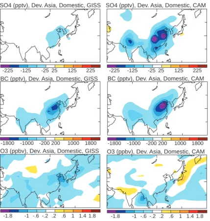
Annual average local reductions take place for all the major pollutants in both mod-els in response to reductions in emissions from developing Asia domestic fuel burning (Fig. 1). The reductions have a similar spatial pattern in the two models for both BC

20

and sulfate, but the sulfate reductions are much larger in the CAM model than in the GISS model. The total change in particulate is dominated by BC, however, which shows decreases of similar magnitude (∼20% greater in the CAM model) and a nearly identical spatial structure in the two models. If we focus in on the ∼15 000 km2 with the largest reductions (a scale more suitable for pollution studies, yet not so small as

25

(9)

ACPD

8, 11609–11642, 2008

Full Screen / Esc

Interactive Discussion result, with BC concentration reductions roughly an order of magnitude greater than

those for sulfate, and an approximately 20% larger response in the CAM model (Ta-ble 2). Interestingly, the summer surface BC response is larger than the annual mean response in the GISS model, but smaller in the CAM model. Differences in seasonality may be related to variations in how the models simulate convective transport, planetary

5

boundary layer heights, or the transformation of BC from hydrophobic to hydrophilic. Reductions in surface ozone are generally small, with maxima of about 1–1.5 ppbv in both models but a response that extends over a larger, more spatially coherent area in the GISS model (Fig. 1). The surface ozone reduction in the GISS model also shows a distinct local maximum over the Yellow Sea co-located with the largest decreases in

10

surface aerosols, while the CAM model does not. Local ozone reductions increase to levels of 1.5–3.5 ppbv during boreal summer over parts of India, China and Korea in the GISS model, but not in the CAM model. Both these annual and summer increases are statistically significant in the GISS model (all significance is based on the 95% con-fidence level derived from the interannual variability in the simulations). Reductions

15

in surface pollution in areas far from the source region are not generally statistically significant in these simulations.

Decreases in North American industrial/power emissions likewise lead to decreases in local pollutant levels (Fig. 2), with the exception of BC for which no significant changes are seen. Sulfate decreases exhibit very similar spatial structures in the two

20

models, with maxima over the Ohio River valley and reductions of more than 125 pptv extending over most of the Eastern US. In contrast to the response to reduced de-veloping Asia domestic emissions, in this case the GISS sulfate response is ∼20% larger than its CAM counterpart. Ozone reductions are stronger, and extend over a larger area, in the GISS model as well, as they were in the developing Asia

domes-25

tic case, with both models showing the greatest response near the western US Gulf Coast. Again the ozone reductions increase to 2–3.5 ppbv during summer over most of the eastern US in the GISS model, but not in the CAM results. Variations in the ozone response in the two models may be related to differences in incorporation of NMHCs

(10)

ACPD

8, 11609–11642, 2008

Full Screen / Esc

Interactive Discussion and in gas-aerosol coupling (Sect. 2). There is also a significant remote response

over Greenland in the GISS model (1.5–3.5 ppbv summertime decreases), consistent with the strong influence of North American emissions on surface pollution levels there (Stohl, 2006).

In all cases other than North America domestic fuel burning, substantial local

re-5

duction in both annual and summer surface particulate concentrations result from the regional sector emissions reductions (Table 2). They are especially large for the devel-oping Asia domestic case, but are also clear in the response to industrial/power and transportation emissions reductions in both regions. The annual average reductions are generally quite similar in the two models, with differences of <30% for all but one

10

of the statistically significant local responses (Table 2) and in the large-scale aerosol responses (Figs. 1 and 2). Differences between the two models are much greater for seasonal pollutant responses (Table 2). Shifts in oxidants in response to ozone precur-sor emission decreases can sometimes outweigh effects of reductions in sulfur-dioxide emissions, leading to increases in surface sulfate in these emission reduction

experi-15

ments (Table 2). Increases in surface aerosols are not statistically significant, however. Nearly all the aerosols at the surface are in fine mode, so that the PM_2.5 (particulate matter with a mean radius of <2.5 microns) concentration changes are approximately the sum of the BC and sulfate concentration changes given in Table 2 (additional con-tributions from OC and nitrate are comparatively small).

20

4.2 Burdens and aerosol optical depths

We now turn to global scale changes and their potential influence on climate. We begin by examining the global annual average change in the tropospheric burdens of radia-tively active species in the two models (Table 3). The models’ sulfate responses are quite consistent with one another. The largest changes are decreases of the global

sul-25

fate burden by ∼5.5% for reductions in developing Asia industrial/power emissions, by ∼3–4% for reductions in North American industrial/power emissions, and by 0.6–0.8% for reductions in developing Asia domestic fuel burning emissions. The two models’

(11)

ACPD

8, 11609–11642, 2008

Full Screen / Esc

Interactive Discussion changes in the sulfate burden in Tg agree within 5–12% (Table 3). Changes in BC and

ozone burdens are less consistent between the two models. Responses are generally larger in the GISS model. This is especially so for BC burden changes in response to reductions in developing Asia emissions, in which cases the GISS model responses are about a factor of 2.5–3 times greater than the CAM model responses.

5

The climate influence of aerosols is not determined solely by the change in concen-tration or mass, but by the resulting change in optical properties. To examine this, we compare the AOD changes in the two models. The greatest reduction in AOD for the developing Asia perturbations is in the domestic case, while for North American it is in the industrial/power case. The GISS and CAM models show similar AOD decreases

10

for these two perturbation experiments (Fig. 3). The two models’ responses are highly correlated spatially (R=0.8) and the global mean values differ by only 20–30%. For North American industrial/power emissions, the main aerosol change is sulfate. The values of the global mean change in sulfate AOD in the two models are within 30%, and the spatial correlation of the AOD decreases is R=0.9 (the total AOD change is so

15

strongly dominated by sulfate in this case that the response pattern and magnitude are virtually identical to those shown in Fig. 3). The models are even consistent in showing a reduction in sulfate AOD over East Asia due to decreases in oxidants stemming from reduced emissions of ozone precursors in North America. Note that the ∼30% differ-ence in the AOD change between the models is larger than the ∼10% differdiffer-ence in the

20

burden change.

For developing Asia domestic sector emission reductions, BC is the largest aerosol change (in absolute or percentage terms). As noted, the total AOD changes in the two models are similar (Fig. 3). In this case, the contribution to AOD from BC was not available for the CAM model, though total carbonaceous aerosol AOD changes

25

were recorded. The AOD change from BC+OC is −0.0013 in the GISS model and −0.0008 in the CAM model. Much of the 47% greater response in the GISS model appears to be due to a larger effect of OC on the AOD (the GISS AOD change due to OC is −0.0008, as large as the total AOD change from BC+OC in the CAM model).

(12)

ACPD

8, 11609–11642, 2008

Full Screen / Esc

Interactive Discussion However, there may be important differences in the AOD change due to BC as well,

to which the greater BC burden change in the GISS model certainly contributes. Also in the developing Asia domestic case, the AOD change from sulfate is twice as large in the CAM model as in the GISS model (−0.0004 and −0.0002, respectively). This is consistent with the sulfate burden changes (Table 2), though AOD shows a larger

5

relative difference than burden. Conversely, the BC burden changes differ much more than the AOD changes due to carbonaceous aerosols. This highlights how AOD (and RF) depend on several factors, including aerosol optical properties, water uptake, and vertical distribution, as well as on aerosol mass.

Hence for industrial/power sector emissions reductions, where sulfate is the

dom-10

inant aerosol change, the total aerosol response appears to be reasonably robust across these two models in terms of the burden change and the magnitude and spatial pattern of AOD changes. For the domestic fuel burning sector emissions reductions, where BC has the greatest impact on climate, the aerosol changes are less robust be-tween the two models for either the decrease in atmospheric mass of BC or the AOD

15

reductions due to individual aerosol species. Nevertheless, the total AOD change due to reductions in emissions from this sector is fairly similar in both magnitude and spatial pattern (Fig. 3). Although decreases in absorbing and reflective aerosols will clearly have opposing influences on climate, both models find decreases in sulfate burdens of <1% and substantially greater percentage reductions in BC burdens. Combined with

20

the larger forcing per Tg BC than sulfate, this indicates that RF will be dominated by BC changes and hence that the aerosol forcing is at least qualitatively consistent in these models, especially in its spatial structure (see also Sect. 4.3).

4.3 Radiative forcing

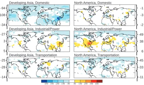
RF was calculated in the GISS model (Fig. 4), and is, unsurprisingly, closely related

25

to the AOD changes. The spatial pattern of the AOD changes is in fact highly corre-lated (R=0.7) with the areas of substantial (greater than ±100 mW/m2) RF in the GISS model in the cases where the net RF from short-lived species emissions is greatest:

(13)

ACPD

8, 11609–11642, 2008

Full Screen / Esc

Interactive Discussion developing Asia domestic and North American industrial/power (Fig. 3 versus Fig. 4).

Correlation values either with total RF, as in Fig. 4, or with aerosol RF only are within 0.1 of each other, emphasizing the dominance of aerosol forcing over ozone forcing in the largest local RF changes. Hence the AOD serves as a useful rough indica-tor of RF, especially for regions where the forcing is greatest. In the industrial/power

5

cases, where AOD changes are largely from sulfate and are in reasonable agreement in the models, both the magnitude and spatial pattern of the RF are also likely to be quite consistent. The standard deviation in global mean RF per unit global mean AOD was 32% in a recent model intercomparison (Schulz et al., 2006), however, so that the total GISS/CAM intermodel variation in RF from aerosols may be slightly greater

10

than that for AOD. Part of the enhanced variability in RF versus AOD (and the discrep-ancy between contributions of individual species to AOD and RF) likely comes from the dependence of forcing on the vertical position of aerosols relative to clouds. As global AOD observations are largely clear-sky, it is difficult to evaluate this aspect of the simulations. Note that the overall aerosol RF uncertainty in both models would be

15

substantially larger including aerosol indirect effects.

In the developing Asia domestic case, the total AOD changes are again compara-ble in magnitude and distribution. However, the contribution from sulfate (a cooling agent) differes substantially, and given the large difference in BC burden changes and in carbonaceous aerosol optical depths (from warming BC and cooling OC), the net

20

RF in the CAM model may have a substantial different magnitude than that in the GISS model. Nonetheless, the relatively consistent response of total AOD in the GISS and CAM models (Fig. 3) suggests that the spatial pattern of RF will be fairly consistent.

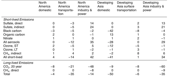
We have evaluated the RF due to reductions in the emissions of short-lived species and their precursors in the GISS model for each individual forcing agent (Table 4).

25

In addition to the direct forcing due to ozone and aerosol changes, we include within the response to short-lived emissions several indirect effects. The indirect effects of aerosols on clouds are thought to be important, but the RF from these effects is quite uncertain, with recent model estimates differing by roughly a factor of five (Penner et

(14)

ACPD

8, 11609–11642, 2008

Full Screen / Esc

Interactive Discussion al., 2006). Hence rather than calculate these forcings directly in the models (which

is computationally expensive as well as uncertain), we estimate their magnitude as in (Fuglestvedt et al., 2008) in which the indirect forcing is simply 1.5 times the direct sulfate forcing over land and 2 times the direct sulfate forcing over oceans, based on (Kvalev ˚ag and Myhre, 2007).

5

We also calculate the methane response to changes in oxidation for all three sets of sector experiments. With methane prescribed at present-day values, changes in mod-eled methane oxidation are due solely to changes in oxidizing agents. Note that the model’s oxidation rate fully captures spatial and seasonal variations. We also include the feedback of methane on its own lifetime (Prather et al., 2001). Finally, we calculate

10

the RF from these indirect methane changes as in (Ramaswamy et al., 2001). We con-sider the direct response of methane to methane emissions changes to be part of the response to emissions of long-lived species (Sect. 5), but include the indirect response of methane to oxidant changes as part of the RF due to short-lived species emissions (as it results from change in emissions of short-lived species and their precursors).

15

Tropospheric ozone changes take place with two distinct timescales. A nearly instan-taneous response, which we term O₃ short-term (ST) occurs as a result of changes in emissions of NO_x, CO, VOCs and SO₂, while a slower response, O₃ long-term (LT) occurs owing to the decadal timescale change in methane due to these same emission changes. The former is calculated by the composition model, while the latter is

esti-20

mated based on the methane response to oxidant changes. As both effects result from change in emissions of short-lived species, both are included in the short-lived portion of Table 4.

We can now examine the contribution of individual species to the RF from emissions perturbations in the GISS model and compare the totals across sectors and regions.

25

The effect of the perturbations is generally larger for developing Asian than North Amer-ican emissions. The only RF from an individual species to reach 10 mW/m2 from a North American perturbation is the sulfate forcing from industrial/power emissions. In contrast, forcings from sulfate, BC, OC and ozone exceed 10 mW/m2 in response to

(15)

ACPD

8, 11609–11642, 2008

Full Screen / Esc

Interactive Discussion perturbations in developing Asia, with the largest response due to decreased BC when

domestic fuel burning emissions are reduced (−42 mW/m2). The total RF due to re-duced short-lived species emissions does not show such a simple relationship between the two regions. The net RF from short-lived species shows comparably large values for both regions for the industry/power generation sector (∼30–40 mW/m2), a larger

5

response to surface transportation for North America, and larger response to domestic fuel burning emissions reductions from developing Asia. The largest positive forcing comes from the industrial/power sector, while the greatest negative forcing comes from developing Asia domestic fuel burning, whose net RF is almost exactly equal to the RF from BC alone. For this sector, the net short-lived emission RF for developing Asia

10

is an order of magnitude larger than for North America, primarily owing to the much larger RF from BC decreases. Conversely, the net RF from short-lived emissions from the surface transportation sector is an order of magnitude larger for North America than for developing Asia, largely due to the difference in the sulfur content of fuels.

Coupling between aerosols and oxidants is clear in the responses. Ozone increases

15

in response to reductions in North American emissions from the domestic or indus-trial/power sectors despite reduced emissions of ozone precursors, especially NO_x for which the industrial/power sector in particular is a large source. This response is due to reductions in SO₂ emissions, which lead to altered radiative fluxes and to reduced heterogeneous nitrogen chemistry on sulfate surfaces (Bell et al., 2005; Liao and

Se-20

infeld, 2005). Analogous results were seen previously for the response of ozone to emissions changes in these sectors in 2030 (Unger et al., 2008). Similarly, sulfate abundances are enhanced in response to reductions in North American surface trans-portation emissions. This occurs because reductions in CO and VOC emissions shift the OH/HO₂ratio toward OH, enhancing gas-phase sulfate formation. This indirect

in-25

fluence of oxidant changes outweighs the direct impact of reduced SO₂ emissions for North American surface transportation, with low-sulfur fuels, but the opposite is true for developing Asia surface transportation emissions (Table 4).

(16)

trans-ACPD

8, 11609–11642, 2008

Full Screen / Esc

Interactive Discussion portation and North America domestic, the RF in response to emissions reduction

from the other four region/sector combinations all show substantial forcing extending over large parts of the Northern Hemisphere (NH) (Fig. 4). This “remote” forcing is in addition to a strongly localized maximum near the source region.

Though forcings were calculated for the GISS model only, we have shown that values

5

for RF from sulfate are likely to be fairly consistent in the two models, indicating that the response to industrial/power sector perturbations is relatively robust. Uncertainties in the response of BC are larger, and could have a substantial effect on RF. Given the dominance of BC in the RF from the domestic fuel burning sector, the net RF may be different in magnitude than that shown here but is likely to be a substantial

10

negative value despite uncertainties. The RF from tropospheric ozone is also uncertain given the large differences in the burden changes in the two models. This will lead to additional uncertainty in the net RF, especially for the surface transportation sector for which the ozone response plays a substantial role, albeit still a small one compared to the influence of aerosols.

15

5 Relative importance of long-lived and short-lived emissions

To explore the total forcing in response to both short- and long-lived species emis-sions reductions from our three sectors, we calculate forcing based on the estimated atmospheric carbon dioxide response to 30% reductions in current emissions from each sector (Table 4). For these calculations, we use sectoral CO₂ emissions from a

20

year 2000 inventory (updated from Olivier and Berdowski (2001)). Atmospheric con-centration changes and the resulting forcing are calculated for the 20-year time horizon, as in the Intergovernmental Panel on Climate Change Third Assessment Report (Ra-maswamy et al., 2001). We believe that using a longer time horizon, such as the 50 or 100 year values also used in that report, is not as useful for comparison with

forc-25

ing from short-lived emissions. As short-lived species responses times are less than a year, use of a many decades long timescale would in a sense be assuming that

(17)

ACPD

8, 11609–11642, 2008

Full Screen / Esc

Interactive Discussion changes in short-lived species precursor emissions took place and then were

main-tained without further modification for another 50 or 100 years, an implausible scenario for most emission changes. For example, mandating a shift from incandescent to more efficient compact fluorescent lighting (CFL) during the next 10 years would lead to a reduction in emissions from power generation relative to continued use of the less

ef-5

ficient technology. While the resulting decrease in CO₂ emissions would indeed still affect atmospheric concentrations a century later, short-lived species emissions result-ing from power generation to provide lightnresult-ing at that time will depend upon the power consumption of 22nd Century lighting equipment, which is unlikely to have any clear re-lationship with a present-day mandate for CFL technology. Hence the 50 and 100 year

10

time horizons are not well-suited to short-lived species emissions. Conversely, using a very short timescale of only a few years or less would overemphasize the response to short-lived species emissions. This response is much faster than the response to long-lived species emissions and can give opposite forcing to the longer term response when looking at all effects (Table 4) or even when looking only at the effect of

short-15

lived precursor emissions (Wild et al., 2001; Fuglestvedt et al., 1999). While the RF response to short-lived species emissions changes is nearly instantaneous (typically days to months for all but those forcing that take place via methane changes), we be-lieve the 20-year time horizon provides a reasonable balance between the effects of long- and short-lived species, is a widely used time horizon in the literature, and is

20

consistent with timescales for air quality policy. Using a longer time horizon would of course give larger relative importance to forcing from long-lived emissions, and vice-versa, and we stress that there is no “best” timescale.

We also calculate the methane response to 30% reductions in regional fossil fuel methane emissions. Emissions are taken from (Fung et al., 1991), with the coal burning

25

source assigned to the power generation sector. As noted previously, simulations did not include interactive methane. We instead calculate the response of methane to the reduced emissions offline, again including the feedback of methane on its own lifetime. We also include the longer-term response of ozone to the methane changes,

(18)

ACPD

8, 11609–11642, 2008

Full Screen / Esc

Interactive Discussion the O₃LT response discussed previously. While strictly speaking this portion of the

O₃LT response should be included under long-term emissions, the values are so small that we group all the O₃ responses together in Table 4. As with the indirect methane response to short-lived precursor emissions, RF is calculated as in (Ramaswamy et al., 2001).

5

Looking at the response to long-lived emissions alone, reductions in North Ameri-can industrial/power generation sector emissions are more than twice as effective in mitigating RF as reductions in the surface transportation sector. The inclusion of the response to emissions of short-lived species alters the comparison markedly, with net total RF from North American surface transportation emissions reductions now more

10

than double that for the North American industrial/power generation sector. For de-veloping Asia, the industrial/power generation sector is by far the most effective for CO₂, and long-lived emissions in general, but the inclusion of the response to short-lived species emissions makes the total net RF from the domestic fuel burning sector larger. Hence the inclusion of RF due to short-lived species emissions reductions

15

strongly shifts the relative importance of emissions from the different economic sec-tors when looking at the 20-year time horizon. Relative to the values due to CO₂ and CH₄(direct), adding the effects of short-lived pollutants increases the forcing from the developing Asia domestic fuel burning sector several times over, enhances the forcing from North American transportation sector emissions by ∼2/3, and reduces the net

20

forcing from industrial/power emissions by ∼50–75%. We reiterate that the timescales for these species differ dramatically, so that short-term and long-term total forcings can be substantially different from one another. This is especially important in the case of industrial/power generation emissions reductions, for which the short and long term forcings are of the opposite sign. They would hence lead to near-term warming

25

but long-term cooling. In the cases where emissions reductions lead to substantial negative forcing via short-lived emissions, developing Asia domestic fuel burning and North America surface transportation, inclusion of the short-lived pollutants dramati-cally enhances near-term climate change mitigation potentials of these sectors relative

(19)

ACPD

8, 11609–11642, 2008

Full Screen / Esc

Interactive Discussion to consideration of the effects of long-lived emissions alone.

6 Discussion and conclusion

The key results for radiative forcing can be summarized as follows. Reductions in surface transportation emissions in North America have a net cooling effect (negative forcing). Negative forcing from long-lived emissions is compounded by negative forcing

5

from short-lived emissions, which results from the net effect of several factors of com-parable magnitude: (1) reductions in BC (which is largely from diesel in this sector), (2) reduction in ozone precursors, which leads to direct reductions in ozone and indirect increases in methane (via reduced oxidation capacity), and (3) decreases in CO and VOC emissions which shift the OH/HO₂ratio toward OH, thereby indirectly leading to

10

increased sulfate (Table 4), as noted previously. Note that the contrasting influence of OH changes on sulfate and methane reflects the difference between the more global methane oxidation and the more regional sulfate oxidation, and implies that these indi-rect effects are quite sensitive to the NOx/(CO+VOCs) emission ratio. Direct impacts

on sulfate via SO₂ emission changes are small owing to the low-sulfur fuel used in

15

North America. Reductions in developing Asia domestic emissions also have a sub-stantial cooling effect via short-lived species emissions which results primarily from reductions in BC and ozone. There is a net decrease in surface particulate and ozone in both cases (Table 2), and hence reducing emissions from these regional sectors offers a way to simultaneously improve human health and mitigate climate warming. In

20

contrast, industrial/power generation emissions have their largest effect on climate via short-lived emissions through sulfate, and hence the net near-term effect of reductions in short-lived species emissions is a positive forcing.

Overall, developing Asia domestic emissions offer the strongest leverage on near-term climate forcing via short-lived species emissions. This is partially a result of their

25

magnitude, and also because they yield a much greater effect via BC changes than via sulfate changes. It also stems from their occurrence at lower latitudes than North

(20)

ACPD

8, 11609–11642, 2008

Full Screen / Esc

Interactive Discussion American (or European) emissions, which enhances their photochemical and

radia-tive impacts as incoming radiation is more abundant at lower latitudes. The GISS and CAM results differ in the magnitude of the total AOD change resulting from the develop-ing Asia domestic sector perturbations by 22%, and this sector/region has the largest influence in both models for both AOD and surface pollution. However, substantial

dif-5

ferences are seen in the two models’ BC change, which dominates the RF in this case, and further work to understand the differences in the aerosol simulations in these mod-els, which are substantial for present-day climatologies as well as for many aspects of the response to perturbations (Shindell et al., 2008), would clearly be useful.

Identical emissions inventories were used in the two models. Emissions can be

10

difficult to quantify, however, especially for carbonaceous aerosols. The inventory of (Bond et al., 2004), for example, has anthropogenic non-biomass burning emissions that are 46% greater for BC and 57% greater for OC for North America than those used here. Similarly, for developing Asia it has 17% less BC and 19% less OC. The 1984 emissions inventory of (Cooke et al., 1999) has much larger (26–77%) carbonaceous

15

aerosol emissions for both regions from fossil fuels than (Bond et al., 2004). Thus the magnitude of the BC and OC forcings calculated here might be fairly different using one of these other inventories. The sign of the net BC+OC effect appears robust, however, as the ratio of emissions of warming BC to cooling OC is within 10% in the three inventories. The lone exception is that the BC/OC ratio is 40% more for North

20

America in (Cooke et al., 1999) compared with (Bond et al., 2004). Even this would simply enhance the net cooling effect seen here in response to reduced emissions from the surface transportation sector there, however, and would not dramatically alter our conclusions. Uncertainties in emissions of sulfate and ozone precursors are generally smaller.

25

The spatial pattern of RF varies substantially between the regional sectors. The RF reduction from decreases in developing Asia domestic emissions extends over much of the NH (Fig. 4). Hence emission changes from this region could in some cases have a larger near-term effect on the RF in other parts of the NH via short-lived

(21)

ACPD

8, 11609–11642, 2008

Full Screen / Esc

Interactive Discussion species emissions than changes in those areas’ own local emissions. Additionally,

re-ductions in transportation or domestic sector emissions cause zonal mean RF due to short-lived species emissions of the same sign throughout the NH, but reductions in industrial/power emissions induce a substantial negative RF in the Arctic while yielding positive RF at lower latitudes in the GISS model (Fig. 4). In this instance, sulfate

re-5

ductions dominate the forcing closer to the emissions at lower latitudes, while BC and ozone are the most important (and roughly comparable) in the Arctic.

The response of AQ, especially particulate, appears to be more robust than the cli-mate forcing across models. This is perhaps not surprising given that RF depends not only on concentrations, but also on such things as water uptake of aerosols, the

verti-10

cal distribution of aerosols and ozone, and the position of ozone and aerosols relative to clouds. Surface ozone amounts are determined by complex, non-linear photochem-istry involving an assortment of NMHCs, so that differences in the models’ chemical mechanisms may play a role in the greater uncertainties in surface ozone than in sur-face aerosols. Additionally, sursur-face pollution levels are particularly important to human

15

health in highly polluted areas, which often cover small areas and are difficult to simu-late correctly in relatively low-resolution global models. Thus although the responses are similar in these two models, they may suffer from biases common to both. Hence our ability to predict both the AQ and RF responses to emissions perturbations has important limitations due to the relatively coarse resolution and simplified aerosol and

20

cloud physics used in current global models.

This work complements prior regional and sectoral perturbations studies examining the response of gas-phase species only (Berntsen et al., 2005; Fuglestvedt et al., 1999; Derwent et al., 2001), aerosol species only (Koch et al., 2007), or both but with a sub-set of the species included here (Unger et al., 2008) or for a single sector for the

25

entire globe (Fuglestvedt et al., 2008). Our analyses suggest that changes in aerosol emissions often have the largest potential leverage on near-term climate forcing via short-lived species emissions. Due to large intermodel differences, the role of ozone changes cannot yet be as clearly assessed, although it is likely that these will have a

(22)

ACPD

8, 11609–11642, 2008

Full Screen / Esc

Interactive Discussion smaller but still important effect both on air quality and climate. Further work is required

to more thoroughly characterize the robustness of these conclusions across a larger number of models and emissions inventories, to explore the impact of aerosol mixing and aerosol indirect effects on clouds more fully, and to examine alternative emissions scenarios considering changes in the mix of sources constituting a given sector and

5

the influence of potential technological changes. The latter could be designed to re-duce emissions of particular pollutants, while not affecting others. Our results for the RF from individual species provide a guide to the potential impact of such technolo-gies. However, we note that these technologies could also have effects on overall fuel consumption by altering the efficiency of a particular process.

10

While there are many difficulties associated with inclusion of short-lived species emissions in international treaties (Rypdal et al., 2005; Bond and Sun, 2005), there are also many tangible near-term benefits in human health, agriculture and forestry that result from improved AQ. Hence a strategy with a dual focus on both AQ and climate change mitigation may present a unique opportunity to engage parties and

na-15

tions not yet fully commited to climate change mitigation for its own sake. Although this is only an initial study, this work suggests that reducing emissions from the developing Asia domestic fuel burning and North America surface transportation sectors may be among the best options for pursuing such a strategy, providing substantial benefits for air quality while simultaneously contributing to climate change mitigation.

20

Acknowledgements. We thank the NASA Atmospheric Chemistry Modeling and Analysis

Pro-gram (ACMAP). JFL was supported by the SciDAC project from the Department of Energy. This research used resources of the National Energy Research Scientific Computing Center, which is supported by the Office of Science of the US Department of Energy under Contract No. DE-AC03-76SF00098. The National Center for Atmospheric Research is operated by the

25

University Corporation for Atmospheric Research under sponsorship of the National Science Foundation.

(23)

ACPD

8, 11609–11642, 2008

Full Screen / Esc

References

Andreae, M. O. and Merlet, P.: Emission of trace gases and aerosols from biomass burning, Global Biogeochem. Cy., 15, 955–966, 2001.

Arellano, A. F. J., Kasibhatla, P. S., Giglio, L., van der Werf, G. R., and Randerson, J. T.: Top-down estimates of global CO sources using mopitt measurements, Geophys. Res. Lett., 31,

5

L01104, doi:10.1029/2003GL018609, 2004.

Bauer, S. E., Mishchenko, M. I., Lacis, A., Zhang, S., Perlwitz, J., and Metzger, S. M.: Do sulfate and nitrate coatings on mineral dust have important effects on radiative properties and climate modeling?, J. Geophys. Res., 112, D06307, doi:10.1029/2005JD006977, 2006. Bauer, S. E., Koch, D., Unger, N., Metzger, S. M., Shindell, D. T., and Streets, D.: Nitrate

10

aerosols today and in 2030: Importance relative to other aerosol species and tropospheric ozone, Atmos. Chem. Phys., 7, 5043–5059, 2007,

http://www.atmos-chem-phys.net/7/5043/2007/.

Bell, N., Koch, D., and Shindell, D.: Impacts of chemistry-aerosol coupling on tropospheric ozone and sulfate simulations in a general circulation model, J. Geophys. Res., 110, D14305,

15

doi:10.1029/2004JD005538, 2005.

Bergamaschi, P., Hein, R., Heimann, M., and Crutzen, P. J.: Inverse modeling of the global CO cycle, 1. Inversion of co mixing ratios, J. Geophys. Res., 105, 1909–1928, 2000.

Berntsen, T. K., Fuglestvedt, J. S., Joshi, M. M., Shine, K. P., Stuber, N., Ponater, M., Sausen, R., Hauglustaine, D. A., and Li, L.: Response of climate to regional emissions of ozone

20

precursors: Sensitivities and warming potentials, Tellus B, 57, 283–304, 2005.

Bond, T., Streets, D., Yarber, K. F., Nelson, S. M., Woo, J.-H., and Klimont, Z.: A technology-based global inventory of black and organic carbon emissions from combustion, J. Geophys. Res., 109, D14203, doi:10.1029/2003JD003697, 2004.

Bond, T. C. and Sun, H.: Can reducing black carbon emissions counteract global warming?,

25

Environ. Sci. Technol., 39, 5921–5926, 2005.

Chung, S. H. and Seinfeld, J. H.: Global distribution and climate forcing of carbonaceous aerosols, J. Geophys. Res., 107, 4407, doi:10.1029/2001JD001397, 2002.

Collins, W. D., Rasch, P. J., Boville, B. A., Hack, J. J., McCaa, J. R., Williamson, D. L., Briegleb, B. P., Bitz, C. M., Lin, S.-J., and Zhang, M.: The formulation and atmospheric simulation of

30

the Community Atmosphere Model: CAM3, J. Climate, 19, 2144–2161, 2006.

(24)

ACPD

8, 11609–11642, 2008

Full Screen / Esc

emission data set for carbonaceous aerosol and implementation and radiative impact in the ECHAM4 model, J. Geophys. Res., 104, 22 137–22 162, 1999.

Dentener, F. D., Stevenson, D. S., Cofala, J., Mechler, R., Amann, M., Bergamaschi, P., Raes, F., and Derwent, R. G.: The impact of air pollutant and methane emissions controls on tropospheric ozone and radiative forcing: CTM calculations for the period 1990–2030, Atmos.

5

Chem. Phys., 5, 1731–1755, 2005,

Derwent, R. G., Collins, W. J., Johnson, C. E., and Stevenson, D. S.: Transient behaviour of tropospheric ozone precursors in a global 3-D CTM and their indirect greenhouse effects, Climatic Change, 49, 463–487, 2001.

10

Fuglestvedt, J., Berntsen, T., Myhre, G., Rypdal, K., and Skeie, R. B.: Climate forcing from the transport sectors, P. Natl. Acad. Sci., 105, 454–458, 2008.

Fuglestvedt, J. S., Berntsen, T. K., Isaksen, I. S. A., Mao, H., Liang, X.-Z., and Wang, W.-C.: Climatic forcing of nitrogen oxides through changes in tropospheric ozone and methane; global 3d model studies, Atmos. Environ., 33, 961–977, 1999.

15

Fung, I., John, J., Lerner, J., Matthews, E., Prather, M., Steele, L. P., and Fraser, P. J.: Three-dimensional model synthesis of the global methane cycle, J. Geophys. Res., 96, 13 033– 13 065, 1991.

Horowitz, L. W., Walters, S., Mauzerall, D. L., Emmons, L. K., Rasch, P. J., Granier, C., Tie, X. X., Lamarque, J.-F., Schultz, M. G., Tyndall, G. S., Orlando, J. J., and Brasseur, G. P.: A

20

global simulation of tropospheric ozone and related tracers: Description and evaluation of mozart, version 2, J. Geophys. Res., 108(D24), 4784, doi:10.1029/2002JD002853, 2003. Koch, D., Bond, T., Streets, D., Bell, N., and van der Werf, G. R.: Global impacts of

aerosols from particular source regions and sectors, J. Geophys. Res., 112, D02205, doi:10.1029/2005JD007024, 2007.

25

Kvalev ˚ag, M. M. and Myhre, G.: Human impact on direct and diffuse solar radiation during the industrial era, J. Climate, 20, 4874–4883, 2007.

Lamarque, J.-F., Kiehl, J. T., Hess, P. G., Collins, W. D., Emmons, L. K., Ginoux, P., Luo, C., and X., T. X.: Response of a coupled chemistry-climate model to changes in aerosol emissions: Global impact on the hydrological cycle and the tropospheric burdens of OH, ozone and

30

NOx, Geophys. Res. Lett., 16, L16809, doi:10.1029/2005GL023419, 2005.

Liao, H. and Seinfeld, J. H.: Global impacts of gas-phase chemistry-aerosol interactions on di-rect radiative forcing by anthropogenic aerosols and ozone, J. Geophys. Res., 110, D18208,

(25)

ACPD

8, 11609–11642, 2008

Full Screen / Esc

doi:10.1029/2005JD005907, 2005.

Metzger, S., Dentener, F., Pandis, S., and Lelieveld, J.: Gas/aerosol partitioning: 1. A compu-tationally efficient model, J. Geophys. Res., 107, 4312, doi:10.1029/2001JD001102, 2002. Metzger, S., Mihalopoulos, N., and Lelieveld, J.: Importance of mineral cations and organics

in gas-aerosol partitioning of reactive nitrogen compounds: Case study based on MINOS

5

results, Atmos. Chem. Phys., 6, 2549–2567, 2006,

Miller, R. L., Cakmur, R. V., Perlwitz, J., Geogdzhayev, I. V., Ginoux, P., Koch, D., Kohfeld, K. E., Prigent, C., Ruedy, R., Schmidt, G. A., and Tegen, I.: Mineral dust aerosols in the NASA Goddard Institute for Space Studies modelE AGCM, J. Geophys. Res., 111, D0208,

10

doi:10.1029/2005JD005796, 2006.

Olivier, J. G. J. and Berdowski, J. J. M.: Global emissions sources and sinks, in: The cli-mate system, edited by: Berdowski, J., Guicherit, R., and Heij, B. J., A.A. Balkema Publish-ers/Swets & Zeitlinger Publishers, Lisse, The Netherlands, 33–78, 2001.

Penner, J. E., Quaas, J., Storelvmo, T., Takemura, T., Boucher, O., Guo, H., Kirkevag, A.,

15

Kristjansson, J. E., and Seland, Ø.: Model intercomparison of indirect aerosol effects, Atmos. Chem. Phys., 6, 3391–3405, 2006,

P ´etron, G., Granier, C., Khattatov, B., Yudin, V., Lamarque, J.-F., Emmons, L., Gille, J., and Edwards, D. P.: Monthly CO surface sources inventory based on the 2000–2001 MOPITT

20

satellite data, Geophys. Res. Lett., 31, L21107, doi:10.1029/2004GL020560, 2004.

Prather, M. J., Ehhalt, D., and Dentener, F. et al.: Atmospheric chemistry and greenhouse gases, in: Climate change 2001, edited by: Houghton, J. T., Cambridge Univ. Press, Cam-bridge, 239–287, 2001.

Ramaswamy, V., Boucher, O., Haigh, J., et al.: Radiative forcing of climate change, in: Climate

25

change 2001, edited by: Houghton, J. T., Cambridge Univ. Press, Cambridge, 349–416, 2001.

Rypdal, K., Berntse, T., Fuglestvedt, J. S., Aunan, K., Torvanger, A., Stordal, F., Pacyna, J. M., and Nygaard, L. P.: Tropospheric ozone and aerosols in climate agreements: Scientific and political challenges, Environ. Sci. Policy, 8, 29–43, 2005.

30

Schmidt, G. A., Ruedy, R., Hansen, J. E., Aleinov, I., Bell, N., Bauer, M., Bauer, S., Cairns, B., Canuto, V., Cheng, Y., Del Genio, A., Faluvegi, G., Friend, A. D., Hall, T. M., Hu, Y., Kelley, M., Kiang, N. Y., Koch, D., Lacis, A. A., Lerner, J., Lo, K. K., Miller, R. L., Nazarenko,

(26)

ACPD

8, 11609–11642, 2008

Full Screen / Esc

L., Oinas, V., Perlwitz, J., Perlwitz, J., Rind, D., Romanou, A., Russell, G. L., Sato, M., Shindell, D. T., Stone, P. H., Sun, S., Tausnev, N., Thresher, D., and Yao, M.-S.: Present day atmospheric simulations using GISS modelE: Comparison to in-situ, satellite and reanalysis data, J. Climate, 19, 153–192, 2006.

Schulz, M., Textor, C., Kinne, S., Balkanski, Y., Bauer, S. E., Berntsen, T., Berglen, T., Boucher,

5

O., Dentener, F., Grini, A., Guibert, S., Iversen, T., Koch, D., Kirkev ˚ag, A., Liu, X., Montanaro, V., Myhre, G., Penner, J., Pitari, G., Reddy, S., Seland, Ø., Stier, P., and Takemura, T.: Radiative forcing by aerosols as derived from the AeroCom present-day and pre-industrial simulations, Atmos. Chem. Phys., 6, 5225–5246, 2006,

10

Shindell, D. T., Faluvegi, G., Unger, N., Aguilar, E., Schmidt, G. A., Koch, D., Bauer, S. E., and Miller, R. L.: Simulations of preindustrial, present-day, and 2100 conditions in the NASA GISS composition and climate model G-PUCCINI, Atmos. Chem. Phys., 6, 4427–4459, 2006,

Shindell, D. T., Faluvegi, G., Bauer, S. E., Koch, D. M., Unger, N., Menon, S., A., Miller, R.

15

L., Schmidt, G. A., and Streets, D. G.: Climate response to projected changes in short-lived species under an A1B scenario from 2000–2050 in the GISS climate model, J. Geophys. Res., 112, D20103, doi:10.1029/2007JD008753, 2007.

Shindell, D. T., Levy II, H., Schwarzkopf, M. D., Horowitz, L. W., Lamarque, J.-F., and Falu-vegi, G.: Multi-model projections of climate change from short-lived emissions due to human

20

activities, J. Geophys. Res., 113, D11109, doi:10.1029/2007JD009152, 2008.

Stohl, A.: Characteristics of atmospheric transport into the Arctic troposphere, J. Geophys. Res., 111, D11306, doi:10.1029/2005JD006888, 2006.

Unger, N., Shindell, D. T., Koch, D. M., and Streets, D. G.: Air pollution radiative forcing from specific emissions sectors at 2030, J. Geophys. Res., 113, D02306,

25

doi:10.1029/2007JD008683, 2008.

Van der Werf, G. R., Randerson, J. T., Collatz, G. J., and Giglio, L.: Carbon emissions from fires in tropical and subtropical ecosystems, Global Change Biol., 9, 547–562., 2003. West, J. J., Fiore, A. M., Horowitz, L. W., and Mauzerall, D. L.: Global health benefits of

miti-gating ozone pollution with methane emission controls, P. Natl. Acad. Sci., 103, 3988–3993,

30

2006.

West, J. J., Szopa, S., and Hauglustaine, D. A.: Human mortality effects of future concentrations of tropospheric ozone, C. r. Geosci., doi:10.1016/j.crte.2007.08.005, 339, 775–783, 2007.

(27)

ACPD

8, 11609–11642, 2008

Full Screen / Esc

Wild, O., Prather, M., and Akimoto, H.: Indirect long-term global radiative cooling from NOx emissions, Geophys. Res. Lett., 28, 1719–1722, 2001.

(28)

ACPD

8, 11609–11642, 2008

Full Screen / Esc

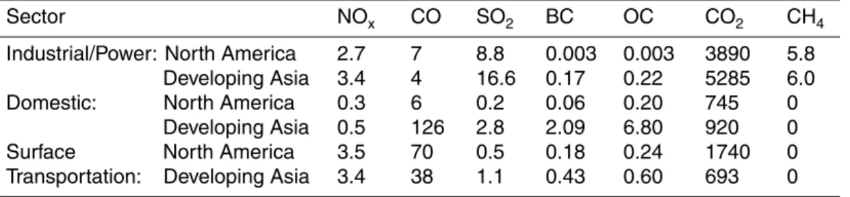
Interactive Discussion Table 1.Regional Annual Average Emissions by Sector (Tg/yr).

Sector NOx CO SO2 BC OC CO2 CH4

Industrial/Power: North America Developing Asia 2.7 3.4 7 4 8.8 16.6 0.003 0.17 0.003 0.22 3890 5285 5.8 6.0

Domestic: North America

Developing Asia 0.3 0.5 6 126 0.2 2.8 0.06 2.09 0.20 6.80 745 920 0 0

Surface North America

Transportation: Developing Asia 3.5 3.4 70 38 0.5 1.1 0.18 0.43 0.24 0.60 1740 693 0 0 Emissions are in Tg N/yr for NOx, Tg S/yr for SO2, in Tg C/yr for BC and OC, and Tg/yr of the species for others. CO2 emissions are from the EDGAR 2000 inventory (updated from (Olivier and Berdowski, 2001)). The industry and power generation sector includes the EDGAR categories industrial, power generation, other transformation sector (refineries, coke ovens, gas works, etc.), non-energy use and chemical feedstocks, oil production, transmission and handling, and cement manufacturing. Surface transportation includes on and off road transport and international shipping. Domestic includes residential and commercial fossil fuel usage and residential biofuel usage. Methane emissions are based on the coal burning source from (Fung et al., 1991). Sources for other emissions are given in Sect. 3.

(29)

ACPD

8, 11609–11642, 2008

Full Screen / Esc

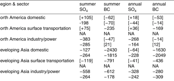
Interactive Discussion Table 2.Local change in surface pollutants (pptv) due to 30% emissions reductions in the given

region and sector

Region & sector summer

SO4 summer BC annual SO4 annual BC

North America domestic [+105]

-198 [−62] [−70] [+18] [−44] [−53] [−14] North America surface transportation [+75]

NA −235NA [+36]NA −169NA

North America industry/power −383

−285 [−47] [21] −268 −164 [−14] [12]

Developing Asia domestic −127

−264 −2430 −1815 [−64] −228 −1630 −2049 Developing Asia surface transportation [−119]

NA −791 NA [−41] NA −436 NA

Developing Asia industry/power −558

−264 −612 −178 −328 −242 −280 −309 Values are averages over comparable areas (∼15 000 km2) containing local maxima with the first row giving results from the GISS PUCCINI model and the second from the CAM MOZART model for each sector. Values in brackets are not statistically significant (significance is based on the 95% confidence level derived from the interannual variability).

(30)

ACPD

8, 11609–11642, 2008

Full Screen / Esc

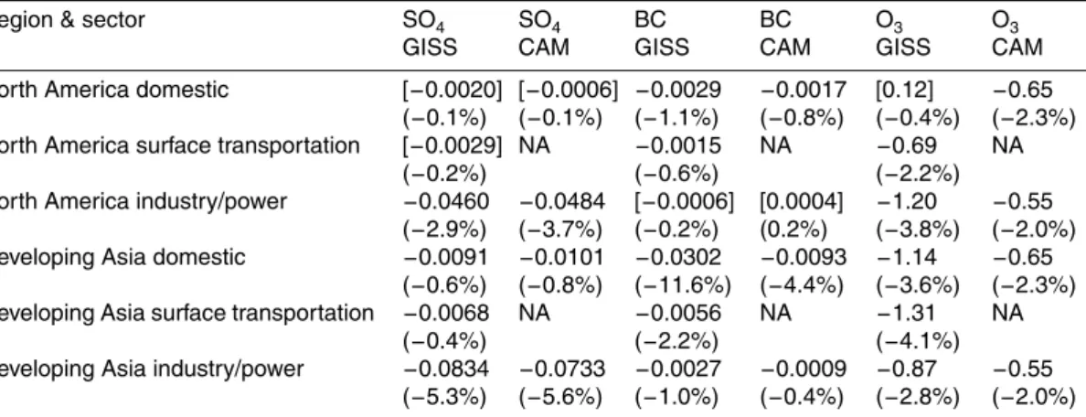
Interactive Discussion Table 3. Tropospheric burden changes due to 30% emissions reductions in the given region

and sector (Tg and %).

Region & sector SO₄ GISS SO₄ CAM BC GISS BC CAM O₃ GISS O₃ CAM North America domestic [−0.0020]

(−0.1%) [−0.0006] (−0.1%) −0.0029 (−1.1%) −0.0017 (−0.8%) [0.12] (−0.4%) −0.65 (−2.3%) North America surface transportation [−0.0029]

(−0.2%) NA −0.0015 (−0.6%) NA −0.69 (−2.2%) NA North America industry/power −0.0460

(−2.9%) −0.0484 (−3.7%) [−0.0006] (−0.2%) [0.0004] (0.2%) −1.20 (−3.8%) −0.55 (−2.0%) Developing Asia domestic −0.0091

(−0.6%) −0.0101 (−0.8%) −0.0302 (−11.6%) −0.0093 (−4.4%) −1.14 (−3.6%) −0.65 (−2.3%) Developing Asia surface transportation −0.0068

(−0.4%) NA −0.0056 (−2.2%) NA −1.31 (−4.1%) NA Developing Asia industry/power −0.0834

(−5.3%) −0.0733 (−5.6%) −0.0027 (−1.0%) −0.0009 (−0.4%) −0.87 (−2.8%) −0.55 (−2.0%)

Values in brackets are not statistically significant (as in Table 2). Values in parentheses are the percent change relative to each model’s own burden in its control run.