Can we explain the trends in European ozone levels?

(1)

HAL Id: hal-00295819

https://hal.archives-ouvertes.fr/hal-00295819

Submitted on 11 Jan 2006

HAL is a multi-disciplinary open access

archive for the deposit and dissemination of

sci-entific research documents, whether they are

pub-lished or not. The documents may come from

teaching and research institutions in France or

abroad, or from public or private research centers.

L’archive ouverte pluridisciplinaire HAL, est

destinée au dépôt et à la diffusion de documents

scientifiques de niveau recherche, publiés ou non,

émanant des établissements d’enseignement et de

recherche français ou étrangers, des laboratoires

publics ou privés.

Can we explain the trends in European ozone levels?

J. E. Jonson, D. Simpson, H. Fagerli, S. Solberg

To cite this version:

J. E. Jonson, D. Simpson, H. Fagerli, S. Solberg. Can we explain the trends in European ozone

levels?. Atmospheric Chemistry and Physics, European Geosciences Union, 2006, 6 (1), pp.51-66.

�hal-00295819�

(2)

www.atmos-chem-phys.org/acp/6/51/ SRef-ID: 1680-7324/acp/2006-6-51 European Geosciences Union

Chemistry

and Physics

Can we explain the trends in European ozone levels?

J. E. Jonson1, D. Simpson1, H. Fagerli1, and S. Solberg2

1_{Norwegian Meteorological Institute, Oslo, Norway} 2_{NILU, Kjeller, Norway}

Received: 27 June 2005 – Published in Atmos. Chem. Phys. Discuss.: 15 August 2005 Revised: 8 November 2005 – Accepted: 9 December 2005 – Published: 11 January 2006

Abstract. Ozone levels in Europe are changing. Emis-sions of ozone precursors from Europe (NOx, CO and non-methane hydrocarbons) have been substantially reduced over the last 10–15 years, but changes in ozone levels cannot be explained by changes in European emissions alone. The ob-served ozone trends at many European sites are only par-tially reproduced by global or regional photochemistry mod-els, and possible reasons for this are discussed.

In order to further explain the European trends in ozone since 1990, the EMEP regional photochemistry model has been run for the years 1990 and 1995–2002. The EMEP model is a regional model centred over Europe but the model domain also includes most of the North Atlantic and the po-lar region. Climatological ozone data are used as initial and lateral boundary concentrations. Model results are compared to measurements over this timespan of 12 years. Possible causes for the measured trends in European surface ozone have been investigated using model sensitivity runs perturb-ing emissions and lateral boundary concentrations. The in-crease in winter ozone partially, and the dein-crease in the mag-nitude of high ozone episodes, is attributed to the decrease in ozone precursor emissions since 1990 by the model. Further-more, the model calculations indicate that the emission re-ductions have resulted in a marked decrease in summer ozone in major parts of Europe, in particular in Germany. Such a trend in summer ozone is likely to be difficult to identify from the measurements alone because of large inter-annual variability.

1 Introduction

Both on a global/hemispheric scale, and regional/local scale, the potential to produce ozone has changed significantly af-Correspondence to: J. E. Jonson

(j.e.jonson@met.no)

ter the onset of industrialization. Both models and measure-ments agree that ozone levels have increased significantly over this period. As discussed below the magnitude and directions of the trends after the mid-1980s are less clear. Since the late 1980s the emissions of ozone precursors, NOx, CO and NMVOC (non-methane volatile organic compounds) have been substantially reduced in most parts of Europe (Vestreng et al., 2004). The reduction in the emissions has resulted in corresponding reductions in the measured con-centrations of these precursor species (Derwent et al., 2003; Solberg, 2004). The anticipated effect of these reductions is that ozone levels in the summer months would be reduced, and that environmentally set thresholds for ozone would be less frequently violated. Reliable surface ozone measure-ments are available since the late 1980s at a number of sites. However, there are large inter-annual variations in ozone lev-els, making it difficult to identify significant trends over the same period (see Sect. 4). The inter-annual variations are mainly determined by meteorological factors such as cloudi-ness, temperature and stability, affecting the ozone produc-tion and residence time in the boundary layer. Further, at many ozone sites sampling background and/or free tropo-spheric air, measured ozone has increased at all seasons, but in particular in winter and spring. The origin, or even ex-tent, of this increase in European background ozone is un-clear (see Sect. 4.1).

This paper discusses a number of factors which affect near-surface ozone levels over Europe, and attempts to quan-tify how far we can account for the observed trends in terms of European emission reductions.

2 Factors affecting European tropospheric ozone trends Although not independent of each other, ozone concentra-tions may be viewed as the sum of a global/hemispheric background concentration and regionally/locally produced

(3)

52 J. E. Jonson et al.: European ozone trends

Table 1. Anthropogenic Emissions (Gg/year) for the EU25 and

Germany. the Czech Republic and United Kingdom separately (Vestreng et al., 2004), and from N. America (UNECE, 2004). N. America includes Canada and USA.

Region 1990 NOx NMVOC CO EU 25 15 991 16 869 61 213 Germany 2845 3591 11 212 Czech Republic 544 441 1257 United Kingdom 2771 2419 7417 N. America 25 775 21 264 97 651 2002 NOx NMVOC CO EU 25 10 988 10 322 33 774 Germany 1499 1478 4311 Czech Republic 318 203 546 United Kingdom 1582 1186 3238 N. America 21 721 17 790 11 1562

ozone. Most of the ozone is believed to originate from the troposphere itself, but a significant fraction is also advected from the stratosphere.

The anthropogenic emissions of ozone precursors (pre-dominantly surface sources) have changed over the last 1– 2 decades. In Europe considerable reductions in emissions have been made since the late 1980s, as can be seen in Ta-ble 1. For NOx and NMVOC, emission reductions are of the order of 30%, and for CO of order 45%, for the EU as a whole, and even greater for some individual countries such as Germany where ozone precursors have been reduced by about 50%.

Emissions from N. America (USA and Canada), being fre-quently upwind from Europe, are also given in Table 1, even though they are outside the model domain. In N. America there is a downward trend of about 15–20% for the emissions of NMVOC and NOxand a slight increase in the emissions of CO over the same period. Emissions are however increasing rapidly in parts of Asia (Streets et al., 2003). There is also a marked upward trend in the emissions from international shipping. Endresen et al. (2003) reports a 1.6% per year in-crease in fuel consumption from shipping between 1996 and 2000.

In the individual countries changes in emissions have been achieved through different sectors. In general the dominant emission sectors have a clear seasonal variation with a winter maximum and a summer minimum. However, sector 7 (road traffic) and sector 8 (other mobile sources and machinery) have small seasonal variations, with a summer maximum. In most countries the percentage contribution from sector 7 and 8 have increased, and as a result emission reductions have been less efficient in summer than in winter. Table 2 lists the

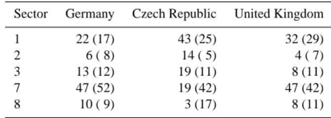
Table 2. Percentage contribution to the national total emissions of

NOxfrom the main sectors in 1990 and 2002 (in brackets) based on the latest available officially reported emissions.

Sector Germany Czech Republic United Kingdom

1 22 (17) 43 (25) 32 (29)

2 6 ( 8) 14 ( 5) 4 ( 7)

3 13 (12) 19 (11) 8 (11)

7 47 (52) 19 (42) 47 (42)

8 10 ( 9) 3 (17) 8 (11)

Notes: Sectors are (1) Combustion in energy and transformation industries; (2) Non-industrial combustion plants; (3) Combustion in manufacturing industry: (7) Road transport; (8) Other mobile sources and machinery.

percentage contributions to NO2emissions in 1990 and 2002 from the dominant sectors for Germany, the Czech Republic and the United Kingdom. The United Kingdom is one of the few countries where the percentage contribution from sec-tor 7 and 8 has decreased. In the Czech Republic the overall emissions in sector 7 and 8 have increased.

One may speculate as to what extent recent changes in the stratospheric ozone layer may have resulted in a reduction in the intrusion of ozone to the troposphere. According to Fusco and Logan (2003) the stratospheric flux of ozone into the troposphere may have decreased by as much as 30% in re-cent years as a result of large declines of lower stratospheric ozone. These changes should be much larger in the south-ern hemisphere as a result of a more pronounced decline in the ozone layer there. There are however indications that the decline in stratospheric ozone has stopped, and that strato-spheric ozone started to recover in the late 1990s (Newchurch et al., 2003, 2004). As a result of global change and changes in stratospheric ozone in particular, circulation patterns may have been altered, which affects the exchange between the stratosphere and troposphere. Measured ozone at mountain tops in Europe is increasing. Kanter et al. (2004) report a pronounced rise in7Be since the mid-1970s. They argue that this is an indication, but not a proof, of an increase in the input from the stratosphere.

Boreal fires in Siberia and N. America may have a marked effect on ozone. Honrath et al. (2004) measured ozone and CO at Mt. Pico on the Azores, and found that ozone levels, el-evated by 15 ppb or more, could often be attributed to boreal fires. Recently it has been shown that there is a strong cor-relation between surface ozone (and other greenhouse gases) and large-scale biomass burning events also at Mace Head (on the Atlantic coast of Ireland) (Simmonds et al., 2005). And, as pointed out by the same authors, Canadian fires have increased steadily over the past two decades according to Stocks et al. (2003).

At least on a regional scale ozone may also be affected by changes in the circulation of the troposphere. There

(4)

are substantial inter-annual variations in tropospheric ozone. Creilson et al. (2003) found a good correlation between the NAO (North Atlantic Oscillation) index and the tropospheric ozone column in the eastern Atlantic in spring, but not for other seasons.

3 Trends in measured ozone precursor levels

The EMEP assessment study showed that the reported emis-sion changes, as discussed in the previous section, have indeed been accompanied by downward trends in the at-mospheric concentrations of these species (Løvblad et al., 2004), although there are many gaps in the data. For NO2the largest reductions in ambient concentrations at rural EMEP sites have been reported in eastern and central parts of Eu-rope (Germany, Czech Republic), with reductions of around 50% between 1990 and 2000. Reductions of around 30% have been reported for NO2for the same period in the Nordic countries, and for Italy, the Netherlands and Switzerland (Løvblad et al., 2004). It should be noted, however, that the number of regional sites with a sufficient monitoring history, and consistent set of measurement data, is rather low.

For NMVOC there is an even lower number of regionally representative monitoring sites, and the data are mostly scat-tered in time. The data do, however, show clear indications of reductions in NMVOC concentration levels during the 1990s (Solberg, 2004). Continuous NMVOC monitoring data from urban background sites in the UK have shown a decrease of 4.5% yr−1and 12% yr−1for individual species during 1994– 2000 (Derwent et al., 2003). Thijsse et al. (1999) showed that there was a shift in the NMVOC composition at Dutch sites during 1990–1997, with an increasing aliphatic/aromatic ra-tio over this period. They related this change to the stronger emission reduction of aromatics caused by the increasing implementation of three-way catalysts in the vehicle fleet. Based on NMVOC measurements at the EMEP monitoring site Moerdijk, which date back to the early 1980s, Roemer (2001a) showed an excellent agreement between observed ethene and acetylene (tracers of car exhaust) and the offi-cial Dutch EMEP road traffic emissions, with an estimated reduction of the order of 50% from 1981 to 1999. Urban studies, e.g. in Denmark (Palmgren et al., 2001), have indi-cated a particular strong decline in the atmospheric benzene concentration due to the reduced benzene content of petrol fuel introduced in the 1990s.

4 Trends in measured ozone levels in the troposphere Trends in ozone are hard to detect because of large inter-annual variations, and therefore long timeseries are needed. For this reason a variety of statistical methods have been used for the meteorological adjustment of ozone trends (Kuebler et al., 2001; Brönnimann et al., 2002; TOR-2, 2003; Tarasova et al., 2004; Ordóñez et al., 2005). The measurements must

be carefully checked for discontinuities and drifts in the data as discussed by Roemer (2001a). Such screening of the data can be made by visual inspection, statistical methods (Schuepbach et al., 2001) or by pairing of neighbouring sites (Roemer, 2001b). Ozone trends are expected to be different in the summer and winter seasons. It is therefore unfortu-nate that most trend studies analyze the measurements with regards to annual mean concentrations.

4.1 Measured Global/Hemispheric trends

Measurements from the early stages of industrialization in-dicate that ozone levels at that time may have been around 10 ppb (Volz and Kley, 1988; Pavelin et al., 1999). There are many problems associated with these early measure-ments, and pre-industrial ozone levels may have been closer to 20 ppbv as measured at Arosa in the 1950s (Staehelin et al., 1994). Studies of ozone-sonde data in the free troposphere (Logan, 1994; Logan et al., 1999; Oltmans et al., 1998) point to a general increase in free tropospheric ozone up to the mid 1980s, and then a mixed picture with many sites/regions showing no significant trend, or even negative trends, after that. In WMO (2002) trends have been calculated including 4 more years (1996–2000), but these additional 4 years did not alter the conclusions significantly. Naja et al. (2003) studied ozone trends at Hohenpeissenberg and Payern and found no positive trends for background ozone in the free troposphere. Studying trends in the last decade at different altitudes in Switzerland, Ord´o˜nez et al. (2004) found a statistically sig-nificant trend of 0.2–0.7 ppb yr−1at elevated sites from au-tumn to spring, at a time when these stations are predom-inantly measuring free tropospheric air. One of the sites (Jungfraujoch, 3580 m a.s.l.) is located close to the ozone sonde station Payern, where no significant trend was reported at this height (Naja et al., 2003). At Zugspitze, 2962 m a.s.l., there is a positive ozone trend between 1990 and 2001, whereas at the nearby, but about 1000 m lower in altitude, site Wank which is more influenced by local effects, there is no significant trend (Kanter et al., 2004).

In the MOZAIC project (http://www.aero.obs-mip.fr/ mozaic/) tropospheric ozone has been measured on a rou-tine basis on commercial aircrafts since 1994. Above Frank-furt and Paris the MOZAIC data indicate trends ranging from about 1.7% yr−1in winter to virtually zero in summer (Zbinden et al., 2005). However, the trend is affected by a high anomaly in 1997–1999 of about 10%. It is unclear as to what extent the trend reported at elevated sites are affected by the same anomaly. Over western Europe and the eastern At-lantic the high ozone levels in the free troposphere in spring-time are correlated with the NAO index in the late 1990s as noted in Sect. 2.

Analysis of the clean sector at surface sites measuring rela-tively unpolluted airmasses (British Isles, Scandinavia) show that there has been an increase in background ozone levels also after the mid 1980s for all seasons, although the increase

(5)

54 J. E. Jonson et al.: European ozone trends is strongest in winter (Solberg, 2003; Roemer, 2001a).

Sim-monds et al. (2004) found that background ozone in the clean oceanic sector measured at Mace Head, Ireland has increased by about 8 ppb from 1987 to 2003.

The difference in trends between the ozone sondes and other measurements such as the MOZAIC data, Mace Head, and mountain sites which often sample free tropospheric air, are not easily reconciled. According to Ord´o˜nez (personal communication) the inconsistency in the trends for sondes versus other measurements may be related to the low sen-sitivity and very low time resolution of these ozone sonde measurements. There may also have been a change in the meteorological limitations as to when to make soundings.

It is unlikely that the increase in ozone in the Atlantic sec-tor at Mace Head (and other surface sites measuring back-ground ozone) is confined to the boundary layer alone, as emissions of ozone precursors have decreased at both sides of the Atlantic. As will be discussed in Sect. 5, this strongly suggests that the increase results from an increase in the free troposphere.

4.2 Measured ozone trends in Europe

Trend analysis of ozone measurements have been mainly re-stricted to northern and western parts of Europe, where rou-tine measurement of ozone first started, and where timeseries are long enough to perform meaningful studies. Overviews of reported trends are given in several publications (Roe-mer, 2001a; TOR-2, 2003; Monks et al., 2003; Solberg et al., 2004). Apart from background sites on the western coast of Europe, trends in surface ozone do not show a uniform pic-ture. However, most sites show substantial downward trends of high ozone (98 or 95 percentiles) over the past 10 to 15 years. For example, in the UK peak ozone concentrations have decreased by about 30% in the period 1986–2001 whilst annual average ozone levels have increased slightly (NEG-TAP, 2001). According to Beilke and Wilson (2000), study-ing the trend at more than 300 ozone sites in Germany be-tween 1990 and 2000, the 99 percentile dropped by 3.3 µg per year (ca. 1.6 ppb yr−1), but with no significant trend for the ozone indicator AOT40, which is a measure of longer-term ozone values (see, e.g. Fuhrer et al., 1997, for definition of AOT40).

Furthermore, at most polluted sites the low ozone per-centiles (mainly winter) are increasing. An important con-tribution to this upward trend is a reduction in the titration by O3+NO reaction in response to the reduction in NOx emis-sions.

5 Calculated trends

5.1 Results from other studies

Model calculations indicate that there has been a substan-tial increase in tropospheric ozone since pre-industrial times,

and that the increase in global free tropospheric ozone has contributed to the increase in surface ozone also in Europe (Berntsen et al., 1997; Lelieveld and Dentener, 2000; Karls-dottir et al., 2000; Hauglustaine and Brasseur, 2001). Fusco and Logan (2003) performed model simulations from 1970 to 1994, and found increasing ozone levels, which they at-tributed to increasing emissions worldwide. In addition to fu-ture projections, Dentener et al. (2004), in a transient global model calculation, compared measured and modeled ozone for 6 surface sites, of which 3 (Westerland, Brotjacklriegel and Schauinsland) are in Europe. None of the sites showed significant measured or calculated trends. Both Brotjackl-riegel and Schauinsland are located at some distance from the coast, and calculated and measured trends should be influ-enced by a combination of background and regional ozone.

Among the global model calculations reported above there is thus a considerable spread in the calculated trend for ozone.

Substantial reductions in modeled peak ozone levels were found comparing results from ten European dispersion mod-els in response to emission changes during the 1990s (Roe-mer et al., 2003). A positive trend in winter ozone, mostly in the 2–4 ppb range in central Europe, was also seen in the model results. This is in good agreement with measurements as noted in Sect. 4.2. Following the decrease in the emissions of ozone precursors, model calculated mean ozone also de-creased in summer by about 10%, but with substantial vari-ability between models. This decrease is not confirmed by the analysis of the measurements. Similar model results were also obtained as part of the EU project TROTREP (Monks et al., 2003). Here particularly large reductions in mean sum-mer ozone were calculated for eastern Europe. In this region there are insufficient measurement data available to verify the model results. In Solberg et al. (2005) it was shown that the changes in the European emissions of ozone precursors in the 1990s have led to significant reductions in measured and calculated surface ozone episodes in the Nordic countries.

As already noted, emissions from international shipping have been increasing at an annual rate of about 1.6% in re-cent years. International shipping has been shown to result in a calculated perturbation of more than 10 ppb in the North Atlantic in the summer (Jonson et al., 2000b; Endresen et al., 2003), with the largest perturbation in the mid Atlantic where NOxlevels are in general low. Calculated effects of interna-tional shipping over the European continent are small (Jon-son et al., 2000b). Such calculations of the effects of ship emissions are however likely to be overestimates because of the non-linearities involved in modeling in low-NOxoceanic areas (Davis et al., 2001; von Glasow et al., 2003). Thus the trend for this source can probably not explain the increase in surface ozone in the clean oceanic sites such as Mace Head, or the increase at mountain tops, mostly in the free tropo-sphere, in winter.

In east Asia ozone and ozone precursors have a greater chance of being lifted into the free troposphere by convection

(6)

compared to other polluted continents, and thereby con-tribute to an increasing trend in the free troposphere through-out the northern mid latitudes. Several studies have tried to quantify the contributions to the ozone levels from different continents or source regions. Derwent et al. (2004) studied the effects of inter-continental transport on ozone by a label-ing technique and by separately reduclabel-ing the anthropogenic emissions in N. America, Europe and Asia of NOxand CO by 50% on an annual basis. The labelling technique indi-cated a contribution of more than 8 ppb from N. America and 4.5 ppb from Asia. Because of non-linearities in the ozone chemistry the tracer labeling technique gives a much higher estimate for the inter-continental contribution than with a 50% reduction in NOxand CO emissions from N. America and Asia. In a similar study by Li et al. (2002) sources in N. America and Asia were separately completely shut off. For the summer months (June, July, August) the calculated contribution from N. America to western parts of Europe by Li et al. (2002) was of the order of 2–3 ppb, whereas the contribution from Asia was of the order of 1 ppb. The ef-fect of inter-continental transport is expected to be relatively smaller in summer. The annual contribution should therefore be larger than just the summer season as studied by Li et al. (2002). Keeping in mind that in the latter study emissions were completely shut off, whereas in Derwent et al. (2004) sources were reduced by 50%, the corresponding results are similar in magnitude.

From the model calculations cited above it seems that the measured increase in background ozone indicated by mea-surements at Mace Head and mountain tops can only be par-tially explained by emission changes in other continents or from international shipping.

5.2 Description of the EMEP model

The EMEP Eulerian Photochemistry model has a polar stereographic projection with a horizontal resolution of 50×50 km2 true at 60◦N and 20 vertical layers below 100 hPa. The model domain is centered over Europe and also includes most of the North Atlantic and the polar region. The EMEP model uses 3-hourly resolution meteorological input data from a dedicated version of the HIRLAM model. The emission data for individual years have been retrieved from the EMEP database (Vestreng et al., 2004). Emis-sions are distributed temporarily and vertically depending on source category. Emissions of NOxand SO2 from interna-tional shipping have been assumed to increase by 2.5% yr−1 from 1990 to 2002. Descriptions and applications of ear-lier versions of the model can be found in Berge and Jakob-sen (1998) and Jonson et al. (1998, 2000a, 2001). Com-pared to earlier model versions the chemical mechanism is now based on the “EMEP scheme” previously described in Simpson et al. (1993); Simpson (1995) and Andersson-Sk¨old and Simpson (1999), but with additional reactions introduced to extend the coverage to acidification and eutrophication

issues. The chemical equations are now solved using the TWOSTEP algorithm tested by Verwer and Simpson (1995). The dry deposition scheme has also been updated. Details of the dry deposition module are given in Simpson et al. (2003a). For ozone the methods have been extensively de-scribed in a series of articles (Emberson et al., 2000, 2001; Simpson et al., 2001, 2003b; Tuovinen et al., 2001, 2004). A thorough description of the model is included in Simpson et al. (2003a), with updates reported in Fagerli et al. (2004).

Initial and lateral boundary conditions (BCs), especially of ozone, represent key inputs to the EMEP model. For ozone, these boundary conditions are derived from the 3-D ozone climatology of Logan (1999), modified in order to accommo-date inter-annual variabilities in air masses arriving from the upwind Atlantic region. The modifications are based on the measurements at Mace Head, Ireland as described in Simp-son et al. (2003a), filtered using trajectory analysis to obtain clean-sector O3values. The adjustment (in ppb ozone) in lat-eral boundary concentrations is the same for the whole model domain and at all vertical levels. As ozone mixing ratios gen-erally increase with altitude, the relative adjustment is largest near the surface and becomes very small in the upper free tro-posphere. This procedure was chosen since data from Mace Head cannot in principal be used to correct mid- to upper-tropospheric ozone, and in any case a marked trend is not ev-ident from free tropospheric ozone sonde measurements (see Sect. 4.1). The assumption that all lateral boundaries are af-fected equally by the Mace Head adjustment is rather crude, but works well because the main bulk of the model domain is subject primarily to dominating westerly air movements. The motivation for and effects of the Mace Head correction will be discussed in more detail in a separate paper.

Lateral boundary concentrations are specified for SO2, SO4, NO, NO2 PAN, HNO3, CO, and some VOCs. Con-centrations are specified by annual mean conCon-centrations and a set of parameters for each species describing seasonal, lati-tudinal and vertical, distributions. The lateral boundary con-centrations are taken from a variety of sources described in more detail in Simpson et al. (2003a). In addition we assume trends for NOxand SO2based on emissions from EPA. 5.3 Model runs and sensitivity tests

To explain the mechanisms behind the trends in European ozone (and NO2) levels, we make use of three set of models calculations:

– RefYYYY:

For a year YYYY, emissions from YYYY, meteorol-ogy from YYYY, and monthly ozone boundary condi-tions also for YYYY, through the Mace Head correc-tion. Ref2002 (with YYYY as 2002) is the reference case against which sensitivity tests are conducted. – Em1990:

(7)

6 J. E. Jonson and D. Simpson and H. Fagerli and S. Solberg: European ozone trends

– AvgBC:

Emissions from 2002, meteorology from 2002, and the same monthly ozone boundary conditions each year, which consist of a ‘10-year’ climatology based upon the monthly averages of the data-sets over the period 1990– 2000. (Same as Ref2002, except for BCs)

The ‘Ref’ runs corresponds to normal EMEP model usage and represents our best estimate of emissions, meteorology and BCs. The Em1990 case is used to explore the effect of emission changes only. The AvgBC case is used to explore what happens when interannual variability and trends are ig-nored. (The AvgBCs where chosen rather than 1990 BCs as this is more robust than BCs from a single year. )

For the ‘Ref’ series of runs, model calculations with the EMEP photochemistry model have been made for 1990 and for the years 1995 to 2002. The years 1991–1994 are not included in the calculations as we have no meteorological input data for these years. Emissions for the relevant years are from Vestreng et al. (2004).

5.4 Calculated and measured NO2in the European

bound-ary layer, 1990 to 2002

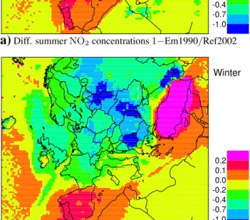
In Figure 1 the differences in calculated NO2concentrations

are shown for a) summer and b) winter. In winter (January, February) calculated reductions in NO2 are of the order of

30% or more in central and eastern Europe. In summer (June, July, August) reductions are in general smaller, and in some areas such as in Hungary and in particular the Czech Republic, absent or even positive. In the Iberian peninsula and in Turkey NOx emissions have increased, resulting in

higher concentrations. Concentrations have also increased over many ocean areas, consistent with increasing ship emis-sions over this period.

The NO2 measurements used in this paper are daily

sam-ples using either absorbing solution (Germany, Poland) or NaI impregnated glass sinters (Sweden, Norway, Hungary). Both of these methods are more selective for NO2than the

standard NOxmonitor. There can be some interference with

HNO2, but the concentration level of this compound is

ex-pected to be relatively low. Unfortunately, there is a clear bias towards northwest Europe in the location of the sites, so we cannot evaluate changes in many other parts of Europe.

Figure 2 depicts measured and calculated NO2 levels for

13 European sites measuring NO2 for all relevant years, for

(a) the ensemble of all 13 sites, (b) the 3 German sites, (c) the 8 northern European sites, and (d) the 2 eastern Euro-pean sites. There is a tendency for the model to overpredict winter concentrations especially in the Nordic areas, and to underpredict summer concentrations of NO2, but in general

the levels and seasonal patterns of NO2are well captured by

the model. Trends for the same site ensembles as in Figure 2, and for the 13 individual sites, are listed for all 4 seasons in Table 3. As for the model calculations, measured trends

a)

Diff. summer NO2concentrations 1_{−Em1990/Ref2002}

b)

Diff. winter NO2concentrations 1_{−Em1990/Ref2002}

Fig. 1. Fractional difference in calculated NO2concentrations in

a) summer and b) winter. Ref2002 is the reference model run. Em1990 is the same model run repeated with 1990 emissions.

are derived disregarding the years 1991–1994. In general the measured trends are reasonably well reproduced by the model. However, both calculated and measured trends may be biased by the use of only one year (1990) at the begin-ning of the period. Observed wintertime NO2seems to have

decreased by 1–2 µg Nm−3over the European stations from

1990 to 2000, but less in northern Europe, where levels are much lower. As in Figure 1, summertime trends are smaller, and in some areas even absent both for measured and calcu-lated NO2. The small calculated trends in northern Europe

can partially be attributed to the assumed increase in emis-sions from international shipping, which represent a signifi-cant fraction of NOxemissions in that region.

A likely explanation for the smaller measured and calcu-lated reductions in NO2 in summer, and the calculated

in-crease in the Czech Republic as shown in Figure 1a in par-ticular, is that emissions from stationary sources, peaking in winter, have decreased whereas changes in mobile sources (sector 7 and 8, see Table 2) , with virtually constant emis-sions throughout the year, are smaller, and in some areas even Atmos. Chem. Phys., 0000, 0001–16, 2005 www.atmos-chem-phys.org/0000/0001/ Fig. 1. Fractional difference in calculated NO2 concentrations in

(a) summer and (b) winter. Ref2002 is the reference model run.

Em1990 is the same model run repeated with 1990 emissions.

monthly ozone boundary conditions also for 2002, through the Mace Head correction. (Same as Ref2002, except for emissions)

– AvgBC:

Emissions from 2002, meteorology from 2002, and the same monthly ozone boundary conditions each year, which consist of a “10-year” climatology based upon the monthly averages of the data-sets over the period 1990–2000. (Same as Ref2002, except for BCs) The “Ref” runs corresponds to normal EMEP model usage and represents our best estimate of emissions, meteorology and BCs. The Em1990 case is used to explore the effect of emission changes only. The AvgBC case is used to explore what happens when interannual variability and trends are ig-nored. (The AvgBCs where chosen rather than 1990 BCs as this is more robust than BCs from a single year. )

For the “Ref” series of runs, model calculations with the EMEP photochemistry model have been made for 1990 and for the years 1995 to 2002. The years 1991–1994 are not included in the calculations as we have no meteorological input data for these years. Emissions for the relevant years are from Vestreng et al. (2004).

5.4 Calculated and measured NO2in the European bound-ary layer, 1990 to 2002

In Fig. 1 the differences in calculated NO2 concentrations are shown for a) summer and b) winter. In winter (Jan-uary, February) calculated reductions in NO2are of the order of 30% or more in central and eastern Europe. In summer (June, July, August) reductions are in general smaller, and in some areas such as in Hungary and in particular the Czech Republic, absent or even positive. In the Iberian peninsula and in Turkey NOx emissions have increased, resulting in higher concentrations. Concentrations have also increased over many ocean areas, consistent with increasing ship emis-sions over this period.

The NO2measurements used in this paper are daily sam-ples using either absorbing solution (Germany, Poland) or NaI impregnated glass sinters (Sweden, Norway, Hungary). Both of these methods are more selective for NO2than the standard NOxmonitor. There can be some interference with HNO2, but the concentration level of this compound is ex-pected to be relatively low. Unfortunately, there is a clear bias towards northwest Europe in the location of the sites, so we cannot evaluate changes in many other parts of Europe.

Figure 2 depicts measured and calculated NO2levels for 13 European sites measuring NO2for all relevant years, for (a) the ensemble of all 13 sites, (b) the 3 German sites, (c) the 8 northern European sites, and (d) the 2 eastern Euro-pean sites. There is a tendency for the model to overpredict winter concentrations especially in the Nordic areas, and to underpredict summer concentrations of NO2, but in general the levels and seasonal patterns of NO2are well captured by the model. Trends for the same site ensembles as in Fig. 2, and for the 13 individual sites, are listed for all 4 seasons in Table 3. As for the model calculations, measured trends are derived disregarding the years 1991–1994. In general the measured trends are reasonably well reproduced by the model. However, both calculated and measured trends may be biased by the use of only one year (1990) at the begin-ning of the period. Observed wintertime NO2seems to have decreased by 1–2 µg Nm−3_{over the European stations from} 1990 to 2000, but less in northern Europe, where levels are much lower. As in Fig. 1, summertime trends are smaller, and in some areas even absent both for measured and calcu-lated NO2. The small calculated trends in northern Europe can partially be attributed to the assumed increase in emis-sions from international shipping, which represent a signifi-cant fraction of NOxemissions in that region.

(8)

a)Europe, 13 stations b)Germany, 3 stations

c)Northern Europe, 8 stations d)Eastern Europe, 2 stations

Fig. 2.Measured and model calculated NO2in µg(N)m−

3_{for the sites (Westerland DE01, Deuselbach DE04, Langenbrügge DE02, Hoburg} SE08, Bredkälen SE05, Vavihill SE11, Osen NO41, K˚arvatn NO39, Tustervatn NO15, Skre˚adalen NO08, Birkenes NO01, Jarczew PL02, K-puszta HU02) upper left, for the 3 German sites (Westerland, Deuselbach, Langenbrügge), upper right, for the Swedish (Hoburg, Bredkälen, Vavihill) and Norwegian sites (Osen, K˚arvatn, Tustervatn, Skre˚adalen, Birkenes) lower left, and the 2 Eastern European sites (Jarczew in Poland and K-puszta in Hungary) lower right. In addition summer and winter trends are shown as straight lines. The years 1991–1994 have not been used deriving the measured trend.

duction seen in Fig. 4b has been canceled out by the changes in BCs.

5.5.2 Em1990 Scenario: Effects on winter ozone

In winter ozone levels are low over the European conti-nent (Figure 5a), largely as a result of the titration reaction NO+O3 →NO2+ O2and the lack of photochemical

activ-ity in most areas. As seen in Fig. 5b, the decrease in NOx,

NMVOC (and other ozone precursors) emissions associated with the Em1990 scenario should have resulted in an increase in ozone levels of the order of 2 ppb or more in most parts of central Europe. This change is in the same range as the ‘Ref’-series of runs, and the observations, as given in Fig. 3c and in Table 4, demonstrating that increases caused by changes in emissions are comparable to increases from BCs in cen-tral Europe.

Over northern Italy, the Em1990 scenario is predicted to result in ozone increases of around 0-2 ppb. This is less than the trends predicted by the ‘Ref’ series of runs, or found in the observations (Fig. 3, Table 4). Results for the Nordic ar-eas are very similar. The Em1990 scenario results in ozone

increases of around 0-2 ppb, which is again less than the trends predicted by the ‘Ref’ series of runs, or the observa-tions. These results suggest that in both of these regions both emissions and BCs play a role in determining the wintertime ozone changes.

5.5.3 Em1990 scenario: Effects on high ozone events The highest ozone events, here defined as the 7 highest ozone days in the year, are shown in Figure 6a. High ozone events are in particular seen in the model calculations in and around the European countries with a Mediterranean coastline, in the countries around the English channel, and in parts of Ger-many. High ozone events are also apparent in the Moscow area. As a result of emission changes from 1990 to 2002 the calculated magnitude of the highest ozone events has been re-duced by 10 ppb or more in large parts of Europe (Figure 6b). In parts of west and central Europe the magnitude has been reduced by as much as 25 ppb. As discussed in section 4.2, changes of this order of magnitude are consistent with down-ward trends of measured high ozone percentiles.

Atmos. Chem. Phys., 0000, 0001–16, 2005 www.atmos-chem-phys.org/0000/0001/

3_{for the sites (Westerland DE01, Deuselbach DE04, Langenbrügge DE02, Hoburg} SE08, Bredkälen SE05, Vavihill SE11, Osen NO41, K˚arvatn NO39, Tustervatn NO15, Skre˚adalen NO08, Birkenes NO01, Jarczew PL02, K-puszta HU02) upper left, for the 3 German sites (Westerland, Deuselbach, Langenbrügge), upper right, for the Swedish (Hoburg, Bredkälen, Vavihill) and Norwegian sites (Osen, K˚arvatn, Tustervatn, Skre˚adalen, Birkenes) lower left, and the 2 Eastern European sites (Jarczew in Poland and K-puszta in Hungary) lower right. In addition summer and winter trends are shown as straight lines. The years 1991–1994 have not been used deriving the measured trend.

Fig. 2.Measured and model calculated NO2in µg(N)m−3for the sites (Westerland DE01, Deuselbach DE04, Langenbrügge DE02, Hoburg SE08, Bredkälen SE05, Vavihill SE11, Osen NO41, K˚arvatn NO39, Tustervatn NO15, Skre˚adalen NO08, Birkenes NO01, Jarczew PL02, K-puszta HU02) upper left, for the 3 German sites (Westerland, Deuselbach, Langenbrügge), upper right, for the Swedish (Hoburg, Bredkälen, Vavihill) and Norwegian sites (Osen, K˚arvatn, Tustervatn, Skre˚adalen, Birkenes) lower left, and the 2 Eastern European sites (Jarczew in Poland and K-puszta in Hungary) lower right. In addition summer and winter trends are shown as straight lines. The years 1991–1994 have not been used deriving the measured trend.

3for the sites (Westerland DE01, Deuselbach DE04, Langenbrügge DE02, Hoburg SE08, Bredkälen SE05, Vavihill SE11, Osen NO41, K˚arvatn NO39, Tustervatn NO15, Skre˚adalen NO08, Birkenes NO01, Jarczew PL02, K-puszta HU02) upper left, for the 3 German sites (Westerland, Deuselbach, Langenbrügge), upper right, for the Swedish (Hoburg, Bredkälen, Vavihill) and Norwegian sites (Osen, K˚arvatn, Tustervatn, Skre˚adalen, Birkenes) lower left, and the 2 Eastern European sites (Jarczew in Poland and K-puszta in Hungary) lower right. In addition summer and winter trends are shown as straight lines. The years 1991–1994 have not been used deriving the measured trend.

In winter ozone levels are low over the European conti-nent (Figure 5a), largely as a result of the titration reaction NO+O3→NO2+ O2and the lack of photochemical

Fig. 2. Measured and model calculated NO2in µg(N)m−3for the sites (Westerland DE01, Deuselbach DE04, Langenbrügge DE02, Hoburg SE08, Bredkälen SE05, Vavihill SE11, Osen NO41, K˚arvatn NO39, Tustervatn NO15, Skre˚adalen NO08, Birkenes NO01, Jarczew PL02, K-puszta HU02) upper left, for the 3 German sites (Westerland, Deuselbach, Langenbrügge), upper right, for the Swedish (Hoburg, Bredkälen, Vavihill) and Norwegian sites (Osen, K˚arvatn, Tustervatn, Skre˚adalen, Birkenes) lower left, and the 2 Eastern European sites (Jarczew in Poland and K-puszta in Hungary) lower right. In addition summer and winter trends are shown as straight lines. The years 1991–1994 have not been used deriving the measured trend.

A likely explanation for the smaller measured and calcu-lated reductions in NO2 in summer, and the calculated in-crease in the Czech Republic as shown in Fig. 1a in partic-ular, is that emissions from stationary sources, peaking in winter, have decreased whereas changes in mobile sources (sector 7 and 8, see Table 2) , with virtually constant emis-sions throughout the year, are smaller, and in some areas even positive.

Overall the decrease in annual NO2 levels is consistent with the emission reductions summarized in Table 1. This is in good agreement with other studies as reported in Sect. 3. 5.5 Calculated ozone over Europe for the years 1990 to

2002

In large parts of Europe the emissions of ozone precursors peaked in the late 1980s. A substantial number of reliable measurements for trend studies are available from about the same time, and we have been able to make use of 54 EMEP sites which had continuous measurements over these years. As already noted in Sect. 4 the interpretation of measured trends are not straight forward. To avoid some of the

prob-lems related to the individual sites we mainly base our con-clusions from the model to measurement comparisons on en-sembles of sites. Figure 3 illustrates calculated and measured monthly averaged daily maximum ozone for (a) all 54 sites, (b) the northern European sites (Norway, Sweden and Fin-land), (c) the German sites, and (d) Ispra (IT04, Italy, the only site with continuous measurements for all the years found for southern Europe), (e) Mace Head (IE31, Ireland), and (f) Deuselbach, (Germany, DE04). No representative sites were found for eastern Europe. In the same figure panels we also show the summer and winter linear trends. Measured and calculated trends for all 4 seasons are listed for several sites (including the ensembles/sites shown in Fig. 3) in Table 4. As for the model calculations, measured trends are derived dis-regarding the years 1991–1994. As for NO2calculated and measured trends may be biased by the use of a single year (1990) at the beginning of the period. The inter-annual vari-ability of ozone from the measurements is well reproduced by the model, with very good agreement for the ensemble of 54 stations, and for Germany in particular. Poorest results are seen for northern Europe, where there is a tendency for the model to under-predict spring ozone. In most areas and

(9)

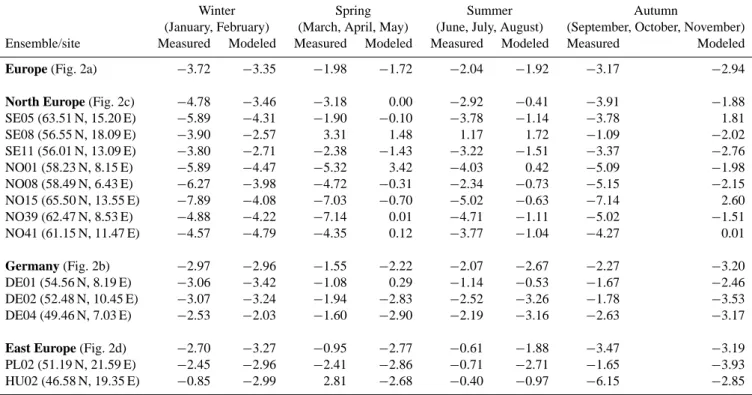
Table 3. Measured and model calculated seasonal NO2trends in µg(N)m−3/yr for the sites/site ensembles shown in Fig. 2. For winter (January, February) and summer (June, July, August) the linear trends listed below are also shown in the same figure. Spring includes data for March, April and May, whereas autumn includes the months September, October and November.

Winter Spring Summer Autumn

(January, February) (March, April, May) (June, July, August) (September, October, November) Ensemble/site Measured Modeled Measured Modeled Measured Modeled Measured Modeled

Europe (Fig. 2a) −3.72 −3.35 −1.98 −1.72 −2.04 −1.92 −3.17 −2.94

North Europe (Fig. 2c) −4.78 −3.46 −3.18 0.00 −2.92 −0.41 −3.91 −1.88

SE05 (63.51 N, 15.20 E) −5.89 −4.31 −1.90 −0.10 −3.78 −1.14 −3.78 1.81 SE08 (56.55 N, 18.09 E) −3.90 −2.57 3.31 1.48 1.17 1.72 −1.09 −2.02 SE11 (56.01 N, 13.09 E) −3.80 −2.71 −2.38 −1.43 −3.22 −1.51 −3.37 −2.76 NO01 (58.23 N, 8.15 E) −5.89 −4.47 −5.32 3.42 −4.03 0.42 −5.09 −1.98 NO08 (58.49 N, 6.43 E) −6.27 −3.98 −4.72 −0.31 −2.34 −0.73 −5.15 −2.15 NO15 (65.50 N, 13.55 E) −7.89 −4.08 −7.03 −0.70 −5.02 −0.63 −7.14 2.60 NO39 (62.47 N, 8.53 E) −4.88 −4.22 −7.14 0.01 −4.71 −1.11 −5.02 −1.51 NO41 (61.15 N, 11.47 E) −4.57 −4.79 −4.35 0.12 −3.77 −1.04 −4.27 0.01 Germany (Fig. 2b) −2.97 −2.96 −1.55 −2.22 −2.07 −2.67 −2.27 −3.20 DE01 (54.56 N, 8.19 E) −3.06 −3.42 −1.08 0.29 −1.14 −0.53 −1.67 −2.46 DE02 (52.48 N, 10.45 E) −3.07 −3.24 −1.94 −2.83 −2.52 −3.26 −1.78 −3.53 DE04 (49.46 N, 7.03 E) −2.53 −2.03 −1.60 −2.90 −2.19 −3.16 −2.63 −3.17

East Europe (Fig. 2d) −2.70 −3.27 −0.95 −2.77 −0.61 −1.88 −3.47 −3.19 PL02 (51.19 N, 21.59 E) −2.45 −2.96 −2.41 −2.86 −0.71 −2.71 −1.65 −3.93

HU02 (46.58 N, 19.35 E) −0.85 −2.99 2.81 −2.68 −0.40 −0.97 −6.15 −2.85

seasons there is very little apparent drift in the model bias over the years (Exceptions are some of the UK sites and Is-pra in northern Italy as discussed in Sect. 5.5.1).

Trends in tropospheric ozone are closely linked to the sea-sonal cycle of ozone. Clean unpolluted sites have a spring ozone maximum and a summer minimum (Monks et al., 2003), whereas polluted (continental) sites are characterized by a broad summer maximum. In particular Mace Head (Fig. 3e), but also the northern European sites (Fig. 3b), are gradually behaving more like unpolluted background sites. At Mace Head the summer and winter trend lines have crossed, resulting in a summer minimum for ozone. In north-ern Europe they are likely to cross in the near future. For both figures spring ozone is seen as the annual peak above the trend lines.

The European ensemble (Fig. 3a and the European en-semble in Table 4) seems to confirm the conclusions from the trend studies already discussed in Sect. 4.2, with ozone levels increasing in winter and less clear or mixed trends in mean ozone for other seasons. Calculated trends and mea-sured trends for different seasons and regions are discussed in more detail below.

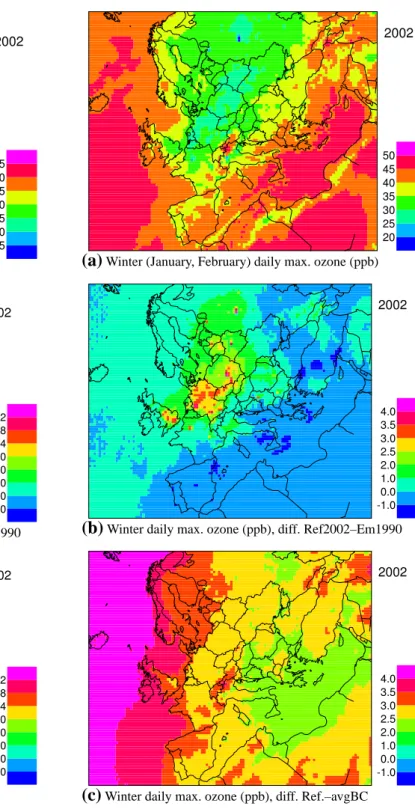
5.5.1 Em1990 scenario: effects on summer ozone

Figure 4a shows mean summer (June, July, August) daily maximum ozone for the base-case simulation for the year 2002 (Ref2002). High ozone levels are in particular seen over the Mediterranean ocean and in northern Italy. Rela-tively high summer ozone is also seen in southern parts of Germany and neighbouring countries.

Figure 4b shows the difference in mean summer ozone levels obtained when using present (year 2002) emissions compared to when using 1990 emissions for the same me-teorological year (2002). Throughout major parts of Europe calculated ozone reductions are in the 5–10 ppb range. Over Turkey and the Iberian peninsula emissions of ozone precur-sors have increased (Vestreng et al., 2004), resulting in small changes or a slight increase in calculated ozone here.

In central Europe, Fig. 4b shows substantial reductions in calculated summer ozone as a result of the Em1990 sce-nario. In southern Germany in particular, reductions in cal-culated ozone of more than 12 ppb are predicted. The re-ductions reflect the substantial rere-ductions in the emissions of ozone precursors in most of Europe, and in particular in Germany, in the same period. However, these ozone reduc-tions are greater than those found in the observareduc-tions or in the base-case (“Ref”) series of model runs for the German sites (Figs. 3c, f, Table 4).

(10)

a)Europe, 54 stations b)Northern Europe, 15 stations

c)Germany, 6 stations d)IT04, Ispra

e)IE31, Mace Head f)DE04, Deuselbach

Fig. 3.Measured and model calculated monthly averaged ozone in ppb. In addition summer and winter trends are shown as straight lines.

For all sites except Mace Head the summer trend lines lies above the winter lines. At Mace Head the trend lines cross and winter ozone is higher than summer ozone for the latter part of the figure. The years 1991–1994 have not been used deriving the measured trend. The top left panel show all sites with continuous ozone measurements for all relevant years, Top right the N. European subset of sites, middle left the German sites, Ispra in N. Italy (middle right), Mace Head (bottom left) and Deuselbach (bottom right). See also Table 4.

surement techniques and procedures. Therefore most fo-cus has been placed on comparison with ensembles of sites, rather than with individual sites, since it has been shown that trend-analysis at any one site is very sensitive to in-strument changes and other factors. Using ensembles we hope to have avoided the most extreme problems of this type. There are large interannual variations in NO2and in ozone

caused by meteorological factors. Calculated and measured trends might be biased by the use of only one year (1990) at the beginning of the period. There are however reasonable

agreements between trends inferred from the transient 1990 to 2002 reference run and differences in NO2and ozone from

the sensitivity tests. Another problem is the robustness of ozone changes against emission change. In a model experi-ment reducing the anthropogenic emissions stepwise in Eu-rope (Monks et al., 2003) it was demonstrated that the largest effects on mean ozone were seen when removing the last 20% of the ozone precursor emissions. Thus reductions in surface ozone caused by more moderate reductions in ozone precursors could easily be masked by inter-annual variability Atmos. Chem. Phys., 0000, 0001–16, 2005 www.atmos-chem-phys.org/0000/0001/ 10 J. E. Jonson and D. Simpson and H. Fagerli and S. Solberg: European ozone trends

Fig. 3. Measured and model calculated monthly averaged ozone in ppb. In addition summer and winter trends are shown as straight lines.

Fig. 3.Measured and model calculated monthly averaged ozone in ppb. In addition summer and winter trends are shown as straight lines.

the sensitivity tests. Another problem is the robustness of ozone changes against emission change. In a model experi-ment reducing the anthropogenic emissions stepwise in Eu-rope (Monks et al., 2003) it was demonstrated that the largest effects on mean ozone were seen when removing the last 20% of the ozone precursor emissions. Thus reductions in surface ozone caused by more moderate reductions in ozone precursors could easily be masked by inter-annual variability Atmos. Chem. Phys., 0000, 0001–16, 2005 www.atmos-chem-phys.org/0000/0001/

Fig. 3.Measured and model calculated monthly averaged ozone in ppb. In addition summer and winter trends are shown as straight lines. For all sites except Mace Head the summer trend lines lies above the winter lines. At Mace Head the trend lines cross and winter ozone is higher than summer ozone for the latter part of the figure. The years 1991–1994 have not been used deriving the measured trend. The top left panel show all sites with continuous ozone measurements for all relevant years, Top right the N. European subset of sites, middle left the German sites, Ispra in N. Italy (middle right), Mace Head (bottom left) and Deuselbach (bottom right). See also Table 4.

Fig. 3. Measured and model calculated monthly averaged ozone in ppb. In addition summer and winter trends are shown as straight lines.

In the UK and Ireland there is a marked difference in model bias from north to south. For Mace Head (IE31) and Strath Vaich Dam (GB15) modeled and measured trends are comparable, whereas for the sites further south there are large negative trends measured, in particular for summer ozone. Measured summer trends in southern parts of the UK are comparable to trends in Germany. This is only partially re-produced by the model.

For the northern Mediterranean area, the Em1990 sce-nario predicts an ozone reduction of ca. 6–12 ppb. This change is similar to that predicted in the “Ref” series of runs

(0.87 ppb yr−1for Ispra), but much greater than the observed trend (0.2 ppb yr−1, Table 4). Results from one site need to be interpreted with caution, so the main conclusion from this study is that for this region the emission trends account for most of the change in modeled ozone between 1990 and 2002.

For the Nordic areas, the Em1990 scenario predicts an ozone reduction of ca. 0–6 ppb. As shown in Fig. 3b and in Table 4 there is virtually no summer trend in this region in either the “Ref”-series of runs or the measurements. As the “Ref”-series include the effects of both emission changes

(11)

Table 4. Measured and model calculated seasonal O3trends in ppb/yr for the sites/site ensembles shown in Fig. 3. For winter (January, February) and summer (June, July, August) trends the linear trends are also shown in the same figure. Spring includes data for March, April and May, whereas autumn includes the months September, October and November. The European ensemble are made up of 13 sites in Great Britain, 11 Austrian sites, 8 Norwegian sites, 6 German sites, 4 Swedish sites, 3 Finnish sites, 2 Belgian sites, 2 Swiss sites and one site in Ireland, Denmark, The Netherlands, Portugal and Italy. N. Europe are made up of a subset of the Norwegian, Swedish and Finnish sites.

Winter Spring Summer Autumn

(January, February) (March, April, May) (June, July, August) (September, October, November) Ensemble/site Measured Modeled Measured Modeled Measured Modeled Measured Modeled

Europe (Fig. 3a) 0.30 0.32 0.11 −0.11 −0.27 −0.36 0.17 0.20

North Europe (Fig. 3b) 0.45 0.49 0.22 −0.01 0.00 −0.12 0.22 0.20

FI22 (66.19 N, 29.24 E) 0.32 0.70 0.00 −0.01 −0.10 0.11 −0.14 0.11 SE11 (56.01 N, 13.09 E) 0.58 0.42 0.02 −0.12 −0.20 −0.34 0.34 0.21 NO41 (61.15 N, 11.47 E) 0.39 0.56 0.18 −0.05 −0.25 −0.18 0.07 0.12 NO42 (78.54 N, 11.53 E) 0.56 0.60 0.56 0.27 −0.09 −0.03 0.16 0.34 NO45 (59.26 N, 10.36 E) −0.04 0.48 −0.30 −0.05 −0.62 −0.16 −0.02 0.28 Germany (Fig. 3c) 0.50 0.30 0.17 −0.28 −0.31 −0.59 0.23 0.15 DE01 (54.56 N, 8.19 E) 0.56 0.35 0.41 −0.11 0.35 −0.24 0.69 0.33 DE03 (47.55 N, 7.54 E) 0.25 0.30 −0.04 −0.54 −0.78 −0.91 0.02 0.03 DE04 (49.46 N, 7.03 E) 0.31 0.28 0.24 −0.01 −0.25 −0.29 0.26 0.21 (Fig. 3f) DE12 (52.51 N, 8.43 E) 1.12 0.49 0.20 −0.23 −0.21 −0.42 0.11 0.17 UK and Ireland 0.13 0.29 −0.06 −0.00 −0.62 −0.22 0.10 0.39 IE31 (53.20 N, 9.54 W) 0.31 0.28 0.24 −0.01 −0.25 −0.29 0.26 0.21 (Fig. 3c) GB15 (57.44 N, 4.46 W) 0.32 0.30 0.09 −0.04 −0.20 −0.30 0.20 0.24 GB37 (57.44 N, 4.46 W) 0.33 0.31 0.09 0.13 −0.87 −0.23 0.12 0.56 GB13 (53.24 N, 1.45 W) 0.04 0.15 −0.35 −0.08 −1.31 −0.62 −0.11 0.37 GB39 (52.17 N, 1.27 E) 0.14 0.33 −0.18 −0.04 −0.93 −0.04 −0.06 0.34 South Europe IT04 (45.48 N, 8.38 E) 0.35 0.46 −0.07 −0.37 −0.20 −0.87 −0.15 0.13 (Fig. 3d) CH02 (46.48 N, 6.57 E) 0.66 0.17 −0.20 −0.51 −0.82 −1.15 0.29 0.44

and BC changes, it seems clear that the effect of the emis-sion reduction seen in Fig. 4b has been canceled out by the changes in BCs.

5.5.2 Em1990 Scenario: effects on winter ozone

In winter ozone levels are low over the European conti-nent (Fig. 5a), largely as a result of the titration reaction NO+O3→NO2+O2 and the lack of photochemical activity in most areas. As seen in Fig. 5b, the decrease in NOx, NMVOC (and other ozone precursors) emissions associated with the Em1990 scenario should have resulted in an in-crease in ozone levels of the order of 2 ppb or more in most parts of central Europe. This change is in the same range as the “Ref”-series of runs, and the observations, as given in Fig. 3c and in Table 4, demonstrating that increases caused

by changes in emissions are comparable to increases from BCs in central Europe.

Over northern Italy, the Em1990 scenario is predicted to result in ozone increases of around 0–2 ppb. This is less than the trends predicted by the “Ref” series of runs, or found in the observations (Fig. 3, Table 4). Results for the Nordic ar-eas are very similar. The Em1990 scenario results in ozone increases of around 0–2 ppb, which is again less than the trends predicted by the “Ref” series of runs, or the observa-tions. These results suggest that in both of these regions both emissions and BCs play a role in determining the wintertime ozone changes.