HAL Id: hal-02331647
https://hal.univ-lorraine.fr/hal-02331647
Submitted on 24 Oct 2019
HAL is a multi-disciplinary open access
archive for the deposit and dissemination of
sci-entific research documents, whether they are
pub-lished or not. The documents may come from
teaching and research institutions in France or
abroad, or from public or private research centers.
L’archive ouverte pluridisciplinaire HAL, est
destinée au dépôt et à la diffusion de documents
scientifiques de niveau recherche, publiés ou non,
émanant des établissements d’enseignement et de
recherche français ou étrangers, des laboratoires
publics ou privés.
Generating variable shapes of salt geobodies from
seismic images and prior geological knowledge
Nicolas Clausolles, Pauline Collon, Guillaume Caumon
To cite this version:
Nicolas Clausolles, Pauline Collon, Guillaume Caumon. Generating variable shapes of salt geobodies
from seismic images and prior geological knowledge. Interpretation, SAGE Publications, 2019, 7 (4),
pp.829 - 841. �10.1190/INT-2019-0032.1�. �hal-02331647�
Interpretation, 7(4): T829–T841, 2019 10.1190/INT-2019-0032.1
Generating variable shapes of salt geobodies from
seismic images and prior geological knowledge
Nicolas Clausolles
1, Pauline Collon
1, and Guillaume Caumon
11Université de Lorraine, CNRS, GeoRessources, F-54000 Nancy, France
Abstract We have developed an implicit method to automatically generate several possible models of salt top surfaces with varying geometries and topologies. This method can be conditioned to available data such as well markers and seismic picks. As seismic imaging of salt is prone to velocity uncertainty and Fresnel zone effects, the input of the method is a seismic image that is segmented into three regions: salt, sediments and uncertain. The uncertain region contains the salt boundary and all the further computations focus within this zone. A monotonic scalar field, ranging from zero on the edge of the certain salt body to one on the maximal possible salt boundary, defines the cumulated probability for a point to be outside the salt body. A random scalar field, also bounded between zero and one, is then used as a threshold for the first scalar field. The salt boundary is implicitly defined by the zero isovalue of the difference between the two fields, and can be further extracted using marching cubes. The random field parameters have a geometrical and topological impact on the simulated salt volumes. They can be adapted to reproduce specific geological features, but their inference remains difficult. The application of the method to the reconstruction of diapir boundaries from a set of partly interpreted sections shows that it is well suited to honor numerous constraining data while proposing different possible structural scenarios in the uninterpreted parts.
Keywords seismic interpretation salt tectonics modeling 3D
Introduction
Recent advances in seismic acquisition methods and processing algorithms enable the imaging of complex geological settings [Jones and Davison, 2014]. The increasing size and quality
of the new seismic data sets have motivated numerous works in seismic interpretation, and especially on the development of automatic interpretation methods. In this global context, a specific attention has been paid to salt tectonics contexts. Salt structures are known, however, to often present challenges for seismic imaging. These challenges stem from three reasons: (1) specific physical properties of evaporites (high velocity and
strong acoustic impedance contrasts with surrounding sedi-ments[e.g.,Fossen,2016]), (2) internal heterogeneity of salt
bodies[e.g.,Jackson and Lewis,2012], and (3) complex
ge-ometries and topologies that develop when salt and surround-ing sediments undergo deformation[e.g.,Hudec and Jackson,
2007]. This leads to a variety of difficulties for seismic
imag-ing, such as poorly illuminated zones, complex travel paths or anisotropy representation[Jones and Davison,2014], which
raises many challenges and uncertainties during structural in-terpretation[Dellinger et al.,2017].
Salt interpretation is usually done in two complementary (but not mandatory) steps: the interpreter first tries to highlight the salt geobodies (or their boundaries) in the seismic data, and then extracts the boundaries by creating three dimensional sur-faces. The most common way to highlight salt is to compute seismic attributes that are sensitive to the image texture. Some authors[e.g.,Gao,2003,Berthelot et al.,2013,Di et al.,2018]
use pixel-based statistical descriptions such as the Gray-Level Co-occurrence Matrix[Haralick et al.,1973] or the Gradient of
Texture[Shafiq et al.,2017]. Other authors focus on
character-izing the local feature orientations. This characterization can be achieved by computing the image gradient using either the gradient covariance matrix[Berthelot et al.,2011] or the
struc-ture tensor[Wu,2016], whose eigen decomposition provides
a measure of the local image anisotropy. Similarly, the reflec-tion dip provides informareflec-tion on the local strata orientareflec-tion [e.g.,Lomask et al.,2007,Halpert and Clapp,2008]. It can
be computed using numerous methods, such as plane-wave destruction filters[Claerbout, 1992] or the ones previously
mentioned for the gradient computation. A third alternative to pixel-based statistical descriptions and local orientations char-acterization consists in characterizing the salt boundaries by solving an edge detection problem[e.g.,Aqrawi et al.,2011,
Amin and Deriche,2015]. As one single attribute may not be
sufficient to highlight the salt boundary in the whole seismic cube, many authors now propose to combine a set of attributes [e.g.,Halpert and Clapp,2008,Berthelot et al.,2013,Di et al.,
2018].
Once the choice of the input attribute(s) has been made, the interpretation of the salt boundary can be seen as a general image segmentation problem. Image segmentation consists in partitioning an input image into different subsets of pixels according to some similarity criterion. In other words, it aims at assigning a label to each image pixel, pixels sharing the same label sharing also some characteristics. This problem has been thoroughly studied in the fields of computer vision and image processing, and numerous methods have been adapted to extract salt boundaries.Lomask et al.[2007],Halpert and Clapp[2008] use normalized cuts image segmentation [Shi and Malik,2000] which is a graph partitioning-based approach.
Other authors use methods based on partial differential equa-tions (PDEs) to fit a surface to the salt boundary.Haukås et al.
[2013,2017] use methods inspired from active-contour
mod-els[Kass et al.,1988] and level sets [Osher and Sethian,1988], Wu[2016] solves a screened Poisson equation to compute an
implicit salt indicator function andWu et al.[2018] extract an
optimal path by solving the eikonal equation. Finally, several authors have also proposed to use various machine learning algorithms[e.g.,Berthelot et al.,2013,Di et al.,2018, Walde-land et al.,2018,Shi et al.,2019].
All these methods aim at automatically determining the “best” possible predicate for the salt boundary. But as noted byLong et al. [2018], the interpreter should keep in mind
that such automatic labeling process can only lead to a first approximation of the salt boundary and not to the exact sur-face. Generating a single deterministic salt geometry can lead to biases in velocity modeling, hydrocarbon trap determina-tion, and reservoir gross rock volume assessment. The topic of seismic interpretation uncertainties has been raised for a long time in classic stratigraphic contexts[e.g.,Abrahamsen,
1993,Thore et al.,2002,Bond et al.,2007], however only a
few papers broach this topic and propose solutions to handle it in the presence of salt.Rojo et al.[2016] discuss the impact of
the attribute selection and tuning on seismic noise reduction along salt boundaries. Most authors also propose to integrate manually picked information to guide the interpretation, ei-ther directly[e.g.,Wu,2016] or during the training phase for
methods relying on classification algorithms[e.g.,Berthelot et al.,2013,Di et al.,2018,Waldeland et al.,2018,Shi et al.,
2019]. Finally, Haukås et al.[2017] propose an interesting
approach to avoid overinterpreting seismic images: they ex-tract surface patches only in well-defined boundary zones, and then smoothly connect the patches in the poorly resolved im-age parts. Such approach remains, however, deterministic as one single interpretation is produced in the end.
To tackle the problem of interpretation bias reduction, we propose a general framework for characterizing the uncertain-ties underlying a seismic image. In practice, it allows for the exploration of different structural scenarios that can be admis-sible considering the imaging uncertainties. This framework is designed in two parts: the first one consists in identifying the image parts in which the interpretation is ambiguous, and the second one focuses on the generation of salt body bound-aries with both variable geometries and topologies. The first part is, therefore, specific to seismic interpretation uncertainty characterization. It has already been investigated by several authors, and numerous works on automatic interpretation can be adapted to address this question (see above references). As it is not the main topic of this paper, we confine the presen-tation to the strategy we retained to model this uncertainty. The second part of the framework, which represents the main contribution of this paper, is more general and can be applied to the modeling of any type of geobodies (salt geobodies, ore geobodies, igneous intrusions, etc.). It addresses the problem of generating complex geobody boundaries while allowing for the integration of data (e.g., seismic picks and well markers) and prior geological knowledge (e.g., type and connectivity of the structures to interpret).
The paper is organized as follows. We first introduce the workflow on a 2D seismic section to provide the reader with a broad overview of the method and the different elements that take part in the modeling process. We then present various simulation results obtained from 3D synthetic data to illustrate the potential of the method, the impact of the different simula-tion parameters, and data condisimula-tioning. We finally discuss the
topics of uncertainty characterization on seismic images, inte-gration of prior geological knowledge and parameter inference from available data.
Method
The most common approach for sampling structural uncertain-ties in geomodeling consists of two steps[e.g.,Abrahamsen,
1993,Lecour et al., 2001]. First, an explicit reference
struc-tural model is built. This reference model can be seen as the “best” possible model considering the limited amount of avail-able data. Then, the different elements of the model (usually horizons and faults) are perturbed around their reference po-sition to sample different possible geometries. This approach presents, however, some limitations. As noted byCaumon et al.
[2007], perturbing an explicit reference model only allows for
exploring geometrical uncertainties and not topological ones. Moreover, perturbing complex surfaces (such as salt geobody boundaries) introduces the risk of generating self-intersecting surfaces[Wellmann and Caumon,2018].
To overcome these limitations, we adopt an implicit mod-eling strategy. Implicit methods are now well-known in geo-modeling and have been widely used in a variety of applica-tions. The seismic grid directly serves as modeling support. The geobody boundaries are represented as a level set of a scalar field[Osher and Sethian,1988]. It prevents classic
topo-logical pitfalls, such as self-intersections and invalid contacts, encountered when perturbing explicit models[Wellmann and Caumon,2018]. It also offers a frame to incorporate
concep-tual knowledge, and especially locally varying anisotropy, into the modeling[e.g.,Martin and Boisvert,2017]. This last point
is addressed later in the paper.
Characterizing the uncertainties
The input of our workflow is a seismic image (Fig. 1.a). The first step consists in identifying the uncertainties in this image. The idea is to discriminate the image parts in which we con-sider the interpretation as sure from those which require more focus. In practice, we propose to classify each pixel of the im-age into one of the following three categories (Fig.1.b): “sed-iments” (in red), “salt” (in blue), and “uncertain” (uncolored). This type of partitioning has also been used byHaukås et al.
[2017] to avoid over-interpreting the image parts in which the
seismic signal is too ambiguous. In our application, the pixels classified as “uncertain” form a volume (referred to as “uncer-tainty envelope”) between the “sediments” and “salt” regions that contains the salt boundary.
In the synthetic examples we present after, the uncertainty envelope is manually defined as we do not have associated seismic images. More details about existing methods that can help to automatically generate the uncertainty envelope are provided in the discussion.
Generating salt boundary interpretations
The next step is to generate salt boundary interpretations in the uncertainty envelope. As stated previously, an interpretation is implicitly defined by a level-set of a scalar field. The generation of this scalar field is inspired by the Object-Distance Simulation (ODSIM) method[Henrion et al.,2010,Rongier et al.,2014].
An interpretation is defined by the combination of two scalar fields: a pseudo-distance field D (Fig. 1.c) and a spatially
Figure 1 Simulating stochastic interpretations of salt boundaries. The input seismic data[a, image fromJackson and Lewis,2012] are
segmented into three categories (b): sediments (red), salt (blue) and uncertain (uncolored). A normalized “distance" field D (c) and a normalized random fieldϕ (d) are then generated in the uncertain region. The salt boundary SB(e, dashed curve) is obtained by extracting
the zero isovalue of the difference between D andϕ (e). Different salt boundaries (f) can be obtained by generating different random fields
(the three realizations share the same distribution and variogram models).
correlated random fieldϕ (Fig. 1.d). The main difference with the ODSIM method is that we perturb the probability of being in the salt body rather than the actual distance to the salt. This approach offers a way to efficiently explore the solution space, and allows for a control of the geometry and topology of the generated boundaries while honoring local salt boundary observations.
The pseudo-distance field D (Fig. 1.c) is a monotonically varying scalar field that ranges from 0 at the contact with the “salt” region and the base of sediments, to 1 at the contact with the external “sediments” region. It represents a relative normalized distance of each sample to salt. In other words, it can be seen as the probability for each sample to be located outside the salt boundary (i.e., to be sediments). This scalar field is obtained by: (1) setting to 0 the value of the samples
in contact with the “salt" region and the base of sediments, (2) setting to 1 the value of the samples in contact with the “sedi-ments" region, and (3) interpolating the intermediate values in the remainder of the “uncertain” region. In this paper, we use the finite difference-based interpolation method proposed byIrakarama et al.[2018] to generate this scalar field.
The second scalar fieldϕ (Fig.1.d) is a spatially correlated random field which is applied to the pseudo-distance field D. The values ofϕ must lie in the same range as the values of
D (between 0 and 1). Two parameters control the random field generation: a distribution model and a spatial correlation model. The distribution model describes the repartition of the values that will be drawn (and must therefore be bounded by 0 and 1). The spatial correlation model describes the local variability of the random field. The choice of the random field
parameters is mainly expert-driven. In this paper, we use a sequential Gaussian simulation (SGS) to generate this random fieldϕ. The spatial correlation model is thus represented by a variogram model.
Once the two scalar fields D andϕ have been generated, we define the salt boundary SB (Fig. 1.e) as the location of
the 0-level surface of the scalar field defined as the difference between D andϕ:
SB:{(t, x, y) | D(t, x, y) − ϕ(t, x, y) = 0}.
As we want to sample structural uncertainties, we need to generate many realizations. In our case, all the realizations share the same pseudo-distance field D. In order to simulate different salt boundaries, we just need to generate one random field per realization. Figure1.f presents three different salt boundaries generated using the same simulation parameters (i.e., distribution and variogram models).
Stochastic generation of salt geobodies
The above workflow is based on several elements: the uncer-tainty envelope, the pseudo-distance field D and the random fieldϕ. Each of these elements requires the definition of some parameters, which raises several questions. How do param-eters impact the realizations? Can we introduce conceptual knowledge into the modeling to reproduce specific geologi-cal features? Can we infer parameters from data and prior knowledge? And overall, can we appraise the different inter-pretations we simulate? The remainder of the paper aims at providing elements to answer these questions. In this section, we use an example of 3D synthetic salt diapir to illustrate the impact of the simulation parameters on the geometry and topol-ogy of the salt boundaries. Using the same example, we then present two examples illustrating how conceptual knowledge can be introduced by an appropriate selection of parameters to reproduce specific geological features. Finally, we explain how local salt observations or interpretations can be integrated in the process.
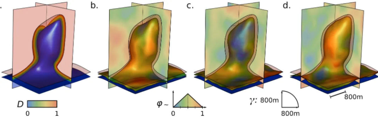
Generating variable salt shapes
Figure2illustrates the generation of different salt boundary ge-ometries. In this example, we consider that the segmentation of the image resulted in a clearly defined salt diapir (below the blue surface in Fig. 2.a). The uncertainties are thus limited to the position of the boundary in the envelope. The distance field D is computed in the uncertainty envelope (Fig.2.a). The SGS parameters used to generate the random fieldϕ are: (1) a triangular distribution model ranging from 0 to 1, with a mode at 0.5, and (2) an isotropic Gaussian variogram model with a range of 800 meters. These parameters are used as “default” parameters in our applications as they allow for the generation of relatively smooth boundaries (the global model size is about 3000 meters) that are centered within the uncer-tainty envelope. It is important to note that the generation of the random fieldϕ is intrinsically prone to statistical biases, due to the relatively large variogram ranges as compared to the uncertainty envelope dimensions. Several strategies can therefore be considered to generate it. The one we selected consists in simulating the random field in the whole seismic image, and keep only the sub-sample corresponding to the un-certainty envelope. Three realizations are presented in Figs.
2.b,2.c, and2.d. Depending on the random field values, the simulated boundaries are generated everywhere in the uncer-tainty envelope and can be either close to salt (blue surface parts) or sediments (red surface parts).
Impact of the simulation parameters
The impact of the parameters used for the simulation of the random fieldϕ is relatively intuitive and can be described in terms of oscillations of the simulated boundary around a ref-erence position. As a reminder, two parameters control the generation ofϕ: a distribution model and a variogram model. The mean of the distribution model determines the refer-ence position of the boundary in the envelope. If the mean is close to zero, the boundary will be statistically close to the “salt” region and, conversely, if the mean is close to one, the boundary will be statistically close to the “sediments” region. It controls therefore the total volume of salt that is simulated. For a given spatial correlation model, the standard deviation of the distribution determines the amplitude of the boundary os-cillations as compared to its reference position: the higher the standard deviation, the larger the amplitude of the oscillations. The principal ranges of the variogram model control the fre-quency of the oscillations around the reference position, and thus the smoothness of the boundary: the larger the ranges, the smoother the boundary. Very short variogram ranges may also trigger the apparition of isolated salt blobs. Figure3 summa-rizes the impact of the parameters on the boundary geometry. It is important to note that the uncertainty envelope, the spatial correlation model and the distribution model all affect the boundary smoothness: the envelope shape controls the global shape of the distance field D (and thus the reference boundary position and its initial shape), the spatial correlation model range determines the global wavelength of the boundary oscillations within this envelope, and the distribution model standard deviation determines how much the boundary can move away from its reference position.
Generating more complex salt shapes
In geology, it is common to have some prior knowledge about the structures being interpreted. Such knowledge can be inferred from many sources of information, such as avail-able data, global geological context, known field analogs, etc. Therefore, an interpreter may want to tune the simulation pa-rameters in order to reproduce specific features. We present here two examples to illustrate how to select the simulation parameters according to a given target salt boundary shape.
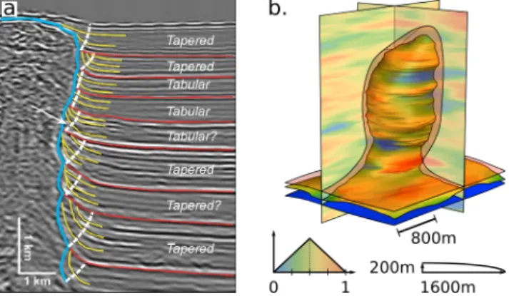
Halokinetic sequences are sedimentary objects that are often associated with salt diapirs. These thin packages of strata are folded upward during the diapir growth, which results in non-conformable relationships between the different packages of strata[Giles and Rowan,2012], and typical cusp-shaped
pat-terns for the salt boundary. Figure4.a illustrates an example of such an interpreted boundary fromGiles and Rowan[2012].
To reproduce these features, we propose to use an anisotropic variogram model, with horizontal ranges higher than the ver-tical range (Fig.4.b). The shorter vertical range reduces the vertical correlation and allows the boundary position to vary more rapidly within the envelop, reproducing the cusp-shaped patterns.
Salt Christmas trees are diapirs with very specific shapes. They are characterized by allochthonous salt “wings” located
Figure 2 Simulating variable salt top boundary geometries. (a) Input data: the “salt” region (in blue), the “sediments” region (in red) and the “uncertain” region (painted with the pseudo-distance field D). The dashed line represents the contact between the external sediments and the uncertainty envelope on the sections. (b), (c) and (d) Three different simulated salt boundaries painted with their respective random fieldsϕ. ϕ follows a triangular distribution, and the variogram model γ is isotropic.
Figure 3 Impact of simulation parameters on the boundary geometry. Each sinusoid represents an idealized boundary within the uncertainty envelope. (a) The distribution model affects the mean position of the boundary. (b) The variogram ranges affect the smoothness of the boundary. The variogram’s principal ranges linearly increase from the left to the right of the uncertainty envelope. Input data from Fig.2.a.
Figure 4 Reproducing halokinetic sequences contact. (a) Example of the typical cusp-shaped patterns observed at the contact between halokinetic sequences (in red) and a salt diapir (in blue). Image and interpretation fromGiles and Rowan[2012]. (b) An example of salt boundary generated using a transversely isotropic variogram model with short vertical range. Input data from Fig.2.a.
between sediment layers and connected to the diapir stem [Mohr et al., 2007]. These wings usually originate from a
former salt glacier stage, when the diapir spread at the surface before being buried again. Figures5.a and5.b illustrate an example of salt glaciers forming such wings around a diapir on seismic sections, extracted fromMohr et al.[2007]. As strata
far from the diapir can generally be imaged and interpreted, we propose to use them to build a relative geologic time func-tion[e.g.,Mallet,2004,Wu and Zhong,2012]. The
equipo-tentials of this function (Fig. 5.c) describe the stratigraphic horizons, but also the diapir wing layout close to the diapir. This information is used during the simulation to locally orient the variogram model axes and reproduce the deposition of the diapir wings over the sediment layers: the “horizontal” axes are aligned along the equipotential surfaces, and the “vertical” axis along the gradient of the stratigraphic function. Combined with anisotropic ranges (very large horizontal ranges and short vertical range), it allows for the simulation of wing-like pat-terns along the diapir flanks. Figure5.d presents a realization example of such a Christmas tree salt diapir.
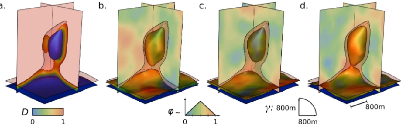
Generating variable salt topologies
For the moment, we have only considered the generation of variable boundary geometries. Depending on the configura-tion of the regions interpreted during the image segmentaconfigura-tion phase, it is also possible to generate salt boundaries with vari-able topologies. In particular, if the “salt” region is made of one basal part and a top teardrop-like part, then both connected and disconnected salt boundaries can be generated. This is illustrated in Fig.6.a: the “salt” region contains a basal layer part, and a salt blob has been isolated above. The intermediate part has, however, been classified as uncertain, which allows for the interpretation of either a diapir stem or a weld. Fig-ures6.b,6.c, and6.d present three examples of simulated salt boundaries, generated using the same random fields as in Figs.
2.b,2.c, and2.d. Depending on the random field values, we generate either connected (Fig.6.d) or disconnected (Figs.6.b and6.c) salt boundaries, which would need to be connected by a weld.
To characterize the topological changes between realiza-tions, the approach ofThiele et al.[2016] could be use. They
propose a framework for characterizing the topological rela-tionships between the different volume entities of a geomodel. In particular, they distinguish between structural and litholog-ical topologies which describe the relations between
respec-tively the different (structural) volumes of conformable strati-graphic units, and the different lithologies (independently of their spatial location). This classification is not perfectly suited for salt tectonics, as diapirs usually have a limited extent at the model scale (they do not cross the whole model) and haloki-netic sequences define complex stratigraphic relations (they can be in the same time conformable in the basin center and unconformable in the diapir vicinity). We consider, however, that it provides an interesting way of describing the different topologies that our method can generate. Our method, in it-self, can generate variable structural topologies (depending on whether the simulated bodies are connected or not). It does not generate variable stratigraphic topologies, as we do not model the sediments. Modeling halokinetic sequences would be, how-ever, an interesting extension of the method and would allow for the generation of variable stratigraphic topologies. Indeed, as the salt boundary geometry varies from one realization to another, modeling different disconnected salt bodies implies modeling different welds, and thus modifying the lithological contacts through the weld.
Conditioning to available data
The method proposed in this paper has the advantage of rest-ing on a simple principle. This makes it easy to adjust to more specific purposes. Especially, it can be constrained to honor var-ious types of geological data. The data conditioning is ensured by constraining the random field generation.
The easiest type of data to handle is punctual information on the salt boundary location (e.g., well markers or deterministic seismic picks indicating the boundary). As the salt boundary is defined by the set of points for which the value of the pseudo-distance field D is equal to the value of the random fieldϕ, such observations can directly be treated as conditioning data for the SGS (by setting at data locations the value of the random fieldϕ to the value of the normalized distance field D). Figure
7illustrates this conditioning. Two well markers (Fig.7.a) are added to the example presented in Fig.6. The simulated salt boundaries (Fig.7.b,7.c and7.d) exhibit variable geometries, but honor the two markers.
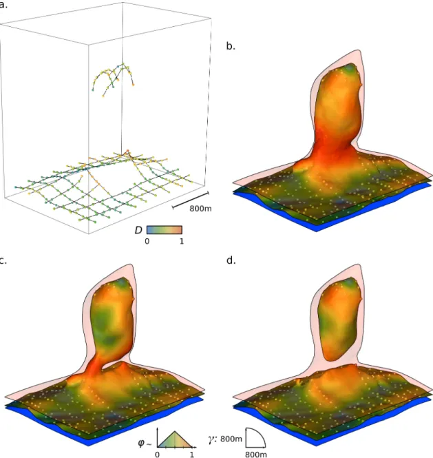
This type of conditioning does not restrict the number of data points that can be taken into account. Our method can, therefore, be applied in cases where some image parts have been interpreted, to reconstruct the boundary in the missing image parts. Figure8presents an example that illustrates this application. We consider that a seismic interpreter has made
Figure 5 Reproducing Christmas tree-like salt diapirs. Example of a salt Christmas tree diapir wing on uninterpreted (a) and interpreted (b) seismic sections. Image and interpretation fromMohr et al.[2007]. (c) Input data from Fig.2.a, with the relative geologic time function used to align the variogram axes displayed on the vertical sections. (d) An example of salt boundary generated using a uniform distribution model and a transversely isotropic variogram model, with a short “vertical” range and larger “horizontal” ranges aligned with the relative time function.
Figure 6 Simulating variable salt top boundary topologies. (a) Input data: the “salt” region (in blue), the “sediments” region (in red) and the “uncertain” region (painted with its pseudo-distance field D). The dashed line represents the contact between the external sediments and the uncertainty envelope on the sections. (b), (c) and (d) Three different simulated salt boundaries, painted with their respective random fieldsϕ.
Figure 7 Conditioning the simulations to well data. (a) Input data from Fig.6.a, with a synthetic well and two markers (white diamonds) indicating the salt boundary position. (b), (c) and (d) Three different simulated salt boundaries (painted with their respective random fields
a fast interpretation of a salt diapir. The interpreter picked the salt boundary every twenty lines, in the regions where it is clearly defined (Fig.8.a). The top of the diapir and the top of the salt layer away from the diapir, which are generally well imaged, are therefore already interpreted. The diapir flanks are, however, poorly resolved and remain to interpret. Figures
8.b,8.c, and8.d present three automatically generated inter-pretations of the possible diapir boundary, which all honor the manually picked samples but exhibit very variable geometries and topologies.
We can also imagine integrating lithological observations (e.g., punctual well log information like “salt” or “sediments”). We do not illustrate this point here, butHenrion et al.[2010]
showed that it only requires the use of a more sophisticated sampling method than direct sampling. They use Gibbs sam-pling[Geman and Geman, 1984] in their application. The
main idea is that the simulated value at conditioning data lo-cation should be in accordance with the observation: if we observed salt, the simulated value should satisfy the condi-tion D− ϕ < 0, and conversely if we are in sediments (then
D− ϕ > 0). The Gibbs sampling ensures that the simulated data still verify the spatial correlation model.
Discussion
In this section, we develop some aspects that have been men-tioned above. In particular, (1) we discuss the problem of the definition of the uncertainty envelope and the pseudo-distance field D, and their impact on the topology of the simulated boundaries; (2) we summarize the different elements about integration of prior knowledge and geological concepts in the modeling; and (3) we develop some points about parameter inference.
Workflow applications and anisotropy modeling
A common question that arises when modeling geological struc-tures is the question of anisotropy modeling. Concerning salt modeling, there are two types of anisotropy: the anisotropy related to the large-scale structures (e.g., salt domes, walls, sheets, etc.) and the anisotropy related to the local features of the salt boundary (e.g., smooth, cusp-shaped, with wings, etc.). It is important to note that, depending on the application, we are not interested in integrating the same level of details into the models. As an example, in geomodeling we are interested in building models that integrate as much information as pos-sible (such as precise halokinetic sequence contacts) in order to make predictions on potential hydrocarbon traps, reservoir heterogeneity, well planning, etc. In seismic imaging, using ve-locity models with such small scale details may, however, lead to more distorted images than using smoother velocity models, as they introduce details that drastically complicate the travel paths. We propose therefore to integrate separately structure-related anisotropy and boundary-structure-related anisotropy into the model. Structure-related anisotropy is handled during the def-inition of the uncertainty envelope, and boundary anisotropy is controlled by the variogram model.
Generation of the uncertainty envelope and
influ-ence on the simulated boundaries
As previously discussed, the topology of the uncertainty en-velope impacts the topology of the simulated salt bodies. As
a reminder, if the initial image segmentation phase produced several independent “salt” regions, then the simulation may produce one or several distinct geobodies. Otherwise, the sim-ulation will produce one single geobody (provided that the variogram principal ranges are large enough to prevent the ap-parition of isolated blobs). The shape of the uncertainty enve-lope also has a direct impact on the geometry of the simulated boundaries, as it controls the shape of the pseudo-distance field
D. It introduces a trend in the interpretations as it defines the “reference” boundary position together with the distribution model mean. We estimate, however, that this trend mainly determines the type of structures that will be interpreted (e.g., salt diapirs, salt walls or allochthonous salt sheets). When in-terpreting seismic images, most of the uncertainties relate to the exact location of the boundaries or the potential salt body connectivities, rather than the type of salt body to interpret. We consider, therefore, that the uncertainty envelope should be as smooth as possible so most of the geometrical properties of the simulated boundary are determined by the simulation parameters rather than the pseudo-distance field D itself.
As it determines the reference position of the boundary, the definition of the uncertainty envelope is a crucial step. Several strategies can be considered to achieve this step. A first solu-tion consists in coupling an automatic interpretasolu-tion method proposed in the literature (see the introduction review) with a confidence criterion. The most straightforward method could be to use the salt indicator function proposed byWu[2016]
and to define the three different categories by thresholding it. As an example,Haukås et al.[2017] use this type of
ap-proach. If enough data points are available (either lithologi-cal or boundary observations), it is also possible to consider building the uncertainty envelope directly from these data, us-ing for example the method proposed byMartin and Boisvert
[2017]. It would provide a good way to integrate locally
vary-ing structural anisotropy. Finally, we can also consider applyvary-ing velocity uncertainty to this envelope[Thore et al.,2002], or
re-migrating it[Osypov et al.,2013,Fomel and Landa,2014]
to account for imaging parameters uncertainty. To go further, it could be interesting to consider methods from the surface reconstruction domain in computer graphics to provide control on the topology of the uncertainty envelope[e.g.,Huang et al.,
2017].
Despite the above, it may not be easy to generate a smooth uncertainty envelope from automatic image segmentation tech-niques. To handle envelopes that would be too irregular, we suggest to use a second envelope that encompasses the first one (thus larger, but smoother). This second envelope is used to generate a smooth distance field D, and the points of the sec-ond envelope that do not belong to the first one (i.e., those that were first classified as “sediments” and then as “uncertain”) can be used as lithological constraints (using a Gibbs sampler) to ensure that the simulated boundaries remain within the initial uncertainty envelope.
Another difficulty a user might face in some configurations consists in generating a pseudo-distance field D allowing for the interpretation of variable salt topologies. As an example, in Fig.1we had to constrain the values of the field D within the diapir stem in order to generate both connected and discon-nected salt bodies. Indeed, as we impose its value to 1 on each side of the stem (at the contact with the “sediments” region), the interpolation populates the stem with values extremely close to 1, which makes the probability of simulating a con-nected salt diapir almost null. To constrain the values within
Figure 8 Sampling variable diapir geometries and topologies while honoring incomplete manual interpretation. (a) Manual seismic picks of the salt boundary (painted with the pseudo-distance field D), used as constraints with the input data from Fig.6. (b), (c) and (d) Three simulated salt boundaries (painted with their respective random fieldsϕ) obtained using the same simulation parameters. The boundaries
the stem, we manually picked several samples within the stem and imposed the distance field values to be equal to 0.5 at the sample location. It is possible to automate this conditioning, for example by extracting the medial axis of the envelope and imposing its value.
To go further, it is possible to impose the topology of the sim-ulated bodies. A potential strategy is to analyze the topology of the pseudo-distance field D to detect the presence of critical points. These points are characterized by a vanishing gradi-ent of D, and idgradi-entify the locations (and the associated values of D) where topological changes will occur when extracting a level set (i.e., when moving from a single to disconnected bod-ies). The values ofϕ can then be adapted to impose a given topology: ifϕ < D at a critical point, disconnected salt bodies are simulated, and conversely ifϕ > D a single salt body is simulated.
Integrating prior knowledge and geological
con-cepts
Knowledge can be integrated either in the uncertainty enve-lope definition or in simulation process, depending on the type of information. The uncertainty envelope constrains the global shape of the structures. Its definition offers a way to integrate information about regional context, such as the regional struc-ture orientations, the type of strucstruc-tures and their connectivity. The distribution model defines the average volume of salt that is generated, and how much the boundary can move away from its reference position in the uncertainty envelope. The variogram model offers a control on the local shape of the boundary. Depending on the application, a user might choose a long range isotropic variogram (to generate smooth bound-aries, Fig.2), or an anisotropic one to reproduce specific pat-terns (Fig. 4). Locally varying anisotropy can be introduced (and especially varying orientations) to reproduce, for example, depositional or salt spreading processes (Fig.5). The choice of the variogram model also determines the influence of punctual data (e.g., well markers ans seismic picks) in the simulation. Choosing a Gaussian model (which is characterized by a large correlation for short distances) ensures that the interpretation in the neighborhood of the data points is consistent with the primary information. The selection of the variogram ranges then offers a way to control the area of influence of the data points.
To go further, it would be interesting to integrate geological concepts in the modeling. The most direct example is maybe the modeling of salt welds. When the simulation produces disconnected salt bodies, we know from a geological point of view that an allochthonous salt body cannot “float” among younger sediments. It has to have been connected to a former salt source through a feeder, whose existence is indicated by the presence of a weld. Modeling welds should be of interest in the oil and gas industry. They play indeed a major role in basin compartmentalization and in the deformation processes that occur at basin scale, and they can severely affect seismic imaging[Jackson and Hudec,2017].
Simulation parameter inference
The definition of the simulation parameters is a key step of the workflow. It should take into account both the geometri-cal and topologigeometri-cal specificities of the salt boundaries to inter-pret, when such characteristics can usually not be observed on
seismic images. Therefore, strategies to calibrate the model parameters need to be developed depending on the type of salt geobodies to be simulated.Henrion et al.[2010] discuss
some aspects of such model parameter calibration using prior geological knowledge. Among the available sources of informa-tion, well data and manual seismic picks can be used to obtain information about the actual salt distribution, geometry and topology. Analogs such as lab experiments[e.g.,Vendeville and Jackson,1992,Dooley et al.,2009], outcrop descriptions [e.g., Ringenbach et al.,2013] or interpreted seismic data sets from
similar geological contexts usually represent another source of information, as they can generally be used together with field data to derive some set of model parameters[Guardiano and Srivastava,1993]. The use of analogs is, however, not directly
possible in our method.
This can be explained by considering the mathematical as-pects of our problem. Let Dper t be the scalar field defined as Dper t = D − ϕ. From a geostatistical point of view, we have
three random fields (D , Dper t, andϕ) related by a linear
com-bination. Considering that D andϕ are independent and in-trinsically second order stationary, we can relate their spatial correlation models:γD= γDper t+ γϕ. This means that,
know-ing the variogram modelsγDandγDper t of D and Dper t, we can
deduce a variogram modelγϕfor the simulated fieldϕ. As we know the pseudo-distance field D, we can compute an experi-mental variogram from it and define an analytical variogram modelγD. The field Dper t, whose variogram model represents
the true variability of the salt boundary, is unknown yet (as the fieldϕ is not known). We might consider using some analog to deduce an analytical modelγDper t. For the analog spatial
correlation model (and thusγDper t) being consistent withγD,
we shall define an uncertainty envelope on the analog. Yet, this is not possible on lab and outcrop analogs. On analog seismic data sets, we can generate an uncertainty envelope. It is, however, not straightforward to estimate the analog bound-ary variability relatively to the envelope, as we only know the zero-level of the analog perturbed distance field, and not this whole field. Moreover, the fields D and Dper tare non-stationary
and exhibit zonal anisotropy, with varying local principal ori-entations. In practice, it is, therefore, complex to define vari-ogram models that actually describe these fields. Finally, the spatial distortion effect induced by the varying width of the uncertainty envelope adds another degree of complexity to the variogram model definition.
Conclusion
The proposed workflow allows for the generation of stochastic interpretations of salt geobody boundaries reflecting seismic imaging uncertainties. It can simulate both connected and dis-connected salt bodies while honoring preexisting geological observations, such as manual seismic picks, well markers and lithological observations. The parameters of the method can be calibrated to reproduce specific geological features; however, quantitative parameter inference remains difficult. To address the impact of geometrical and topological salt interpretation uncertainties, further work should focus on appraising the vari-ous interpretations we generate with our method to inject them back into the seismic processing chain.
Moreover, the workflow is generic and can be used in other types of applications. In particular, it is well suited for the gen-eration of any type of geological body boundaries (salt bodies, ore bodies, igneous intrusions, etc.), even in the presence of
nu-merous constraining data. As an example, it could be of great use for estimating ore deposit extent in mining applications, where numerous data (and especially drillholes) are available.
Acknowledgments
This work was performed in the frame of the RING project (http://ring.georessources.univ-lorraine.fr) at Université de Lorraine. We would like to thank for their support the indus-trial and academic sponsors of the RING-GOCAD Consortium managed by ASGA. We also acknowledge Paradigm-Emerson for the SKUA-Gocad software and development kit. The soft-wares corresponding to this paper are available as the Goscope plugin of SKUA-Gocad and the stand-alone SIGMA library. We would finally like to thank the associate editor B. Wallet, and E. de Kemp, X. Wu and two anonymous reviewers for their work and comments that greatly improved the paper.
References
P. Abrahamsen. Bayesian kriging for seismic depth conversion of a multi-layer reservoir. In Geostatistics Tróia ’92, pages 385–398, 1993. (Cited page2)
A. Amin and M. Deriche. A new approach for salt dome detection using a 3D multidirectional edge detector. Applied Geophysics, 12(3):334–342, 2015.
(Cited page1)
A. Aqrawi, T. Boe, and S. Barros. Detecting salt domes using a dip guided 3D Sobel seismic attribute. In SEG Technical Program Expanded
Ab-stracts 2011, pages 1014–1018. Society of Exploration Geophysicists, 2011.
(Cited page1)
A. Berthelot, A. Solberg, E. Morisbak, and L.-J. Gelius. Salt diapirs without well defined boundaries - a feasibility study of semi-automatic detection.
Geophysical Prospecting, 59(4):682–696, 2011. (Cited page1)
A. Berthelot, A. Solberg, and L.-J. Gelius. Texture attributes for detection of salt. Journal of Applied Geophysics, 88:52–69, 2013. (Cited pages1and2)
C. E. Bond, A. D. Gibbs, Z. K. Shipton, and S. Jones. What do you think this is? "Conceptual uncertainty" in geoscience interpretation. GSA Today, 17 (11):4–10, 2007. (Cited page2)
G. Caumon, A.-L. Tertois, and L. Zhang. Elements for Stochastic Structural Perturbation of Stratigraphic Models. In EAGE Conference on Petroleum
Geostatistics, pages 10–14. European Association of Geoscientists and En-gineers, 2007. (Cited page2)
J. F. Claerbout. Earth soundings analysis: Processing versus inversion, volume 6. Blackwell Scientific Publications Boston, 1992. (Cited page1)
J. Dellinger, A. Brenders, J. Sandschaper, C. Regone, J. Etgen, I. Ahmed, and K. Lee. The Garden Banks model experience. The Leading Edge, 36(2): 151–158, 2017. (Cited page1)
H. Di, M. Shafiq, and G. AlRegib. Multi-attribute k-means clustering for salt-boundary delineation from three-dimensional seismic data. Geophysical
Journal International, 215:1999–2007, 2018. (Cited pages1and2)
T. P. Dooley, M. P. Jackson, and M. R. Hudec. Inflation and deflation of deeply buried salt stocks during lateral shortening. Journal of Structural Geology, 31(6):582–600, 2009. (Cited page10)
S. Fomel and E. Landa. Structural uncertainty of time-migrated seismic images.
Journal of Applied Geophysics, 101:27–30, 2014. (Cited page8)
H. Fossen. Structural geology. Cambridge University Press, 2016.
(Cited page1)
D. Gao. Volume texture extraction for 3D seismic visualization and interpre-tation. GEOPHYSICS, 68(4):1294–1302, 2003. (Cited page1)
S. Geman and D. Geman. Stochastic relaxation, Gibbs distributions, and the Bayesian restoration of images. IEEE Transactions on pattern analysis and
machine intelligence, (6):721–741, 1984. (Cited page8)
K. A. Giles and M. G. Rowan. Concepts in halokinetic-sequence deformation and stratigraphy. Geological Society, London, Special Publications, 363:7–31, 2012. (Cited pages4and6)
F. B. Guardiano and R. M. Srivastava. Multivariate geostatistics: beyond bivariate moments. In Geostatistics Tróia ’92, pages 133–144, 1993.
(Cited page10)
A. Halpert and R. G. Clapp. Salt body segmentation with dip and frequency attributes. Stanford Exploration Project, 136, 2008. (Cited page1)
R. Haralick, K. Shanmugan, and I. Dinstein. Textural features for image clas-sification. In IEEE Transactions on Systems, Man and Cybernetics, volume 3, pages 610–621, 1973. (Cited page1)
J. Haukås, O. Ravndal, B. Fotland, A. Bounaim, and L. Sonneland. Automated salt body extraction from seismic data using the level set method. First
Break, 31(4):35–42, 2013. (Cited page1)
J. Haukås, A. Bounaim, and O. Gramstad. Automated salt interpretation, Part II : Smooth surface wrapping of volume attribute. In SEG Technical
Pro-gram Expanded Abstracts 2017, pages 2076–2080. Society of Exploration Geophysicists, 2017. (Cited pages2and8)
V. Henrion, G. Caumon, and N. Cherpeau. ODSIM: An Object-Distance Simu-lation Method for Conditioning Complex Natural Structures. Mathematical
Geosciences, 42(8):911–924, 2010. (Cited pages2,8, and10)
Z. Huang, M. Zou, N. Carr, and T. Ju. Topology-controlled Reconstruction of Multi-labelled Domains from Cross-sections. ACM Transactions on Graphics, 36(4):76, 2017. (Cited page8)
M. R. Hudec and M. P. A. Jackson. Terra infirma: Understanding salt tectonics.
Earth-Science Reviews, 82(1-2):1–28, 2007. (Cited page1)
M. Irakarama, G. Laurent, J. Renaudeau, and G. Caumon. Finite Difference Implicit Modeling of Geological Structures. In 80th EAGE Conference and
Exhibition 2018, 2018. (Cited page3)
C. A.-L. Jackson and M. Lewis. Origin of an anhydrite sheath encircling a salt diapir and implications for the seismic imaging of steep-sided salt structures, Egersund Basin, Northern North Sea. Journal of the Geological Society, 169 (5):593–599, 2012. (Cited pages1and3)
M. P. Jackson and M. R. Hudec. Salt tectonics: Principles and practice. Cam-bridge University Press, 2017. (Cited page10)
I. Jones and I. Davison. Seismic imaging in and around salt bodies.
Interpre-tation, 2(4):SL1–SL20, 2014. (Cited page1)
M. Kass, A. Witkin, and D. Terzopoulos. Snakes: Active contour models.
Inter-national journal of computer vision, 1(4):321–331, 1988. (Cited page2)
M. Lecour, R. Cognot, I. Duvinage, P. Thore, and J.-C. Dulac. Modelling of stochastic faults and fault networks in a structural uncertainty study.
Petroleum Geoscience, 7:S31–S42, 2001. (Cited page2)
J. Lomask, R. G. Clapp, and B. Biondi. Application of image segmenta-tion to tracking 3D salt boundaries. GEOPHYSICS, 72:P47–P56, 2007.
(Cited page1)
Z. Long, Y. Alaudah, M. A. Qureshi, Y. Hu, Z. Wang, M. Alfarraj, G. AlRegib, A. Amin, M. Deriche, S. Al-Dharrab, et al. A comparative study of tex-ture attributes for characterizing subsurface structex-tures in seismic volumes.
Interpretation, pages T1055–T1066, 2018. (Cited page2)
J.-L. Mallet. Space–time mathematical framework for sedimentary geology.
Mathematical geology, 36(1):1–32, 2004. (Cited page6)
R. Martin and J. Boisvert. Iterative refinement of implicit boundary models for improved geological feature reproduction. Computers and Geosciences, 109:1–15, 2017. (Cited pages2and8)
M. Mohr, J. K. Warren, P. A. Kukla, J. L. Urai, and A. Irmen. Subsurface seismic record of salt glaciers in an extensional intracontinental setting (Late Triassic of northwestern Germany). Geology, 35(11):963–966, 2007.
(Cited pages6and7)
S. Osher and J. A. Sethian. Fronts propagating with curvature-dependent speed: algorithms based on Hamilton-Jacobi formulations. Journal of Computational Physics, 79(1):12–49, 1988. (Cited page2)
K. Osypov, Y. Yang, A. Fournier, N. Ivanova, R. Bachrach, C. E. Yarman, Y. You, D. Nichols, and M. Woodward. Model-uncertainty quantification in seismic tomography: Method and applications. Geophysical Prospecting, 61(6): 1114–1134, 2013. (Cited page8)
J.-C. Ringenbach, J.-F. Salel, C. Kergaravat, C. Ribes, C. Bonnel, and J.-P. Callot. Salt tectonics in the Sivas Basin, Turkey: outstanding seismic analogues from outcrops. First Break, 31(6):93–101, 2013. (Cited page10)
A. L. Rojo, A. Escalono, and L. Schulte. The use of seismic attributes to enhance imaging of salt structures in the Barents Sea. First Break, 34(11): 49–57, 2016. (Cited page2)
G. Rongier, P. Collon-Drouaillet, and M. Filipponi. Simulation of 3D karst con-duits with an object-distance based method integrating geological knowl-edge. Geomorphology, 217:152–164, 2014. (Cited page2)
M. Shafiq, Z. Wang, G. AlRegib, A. Amin, and M. Deriche. A texture-based interpretation workflow with application to delineating salt domes.
Inter-pretation, 5(3):SJ1–SJ19, 2017. (Cited page1)
J. Shi and J. Malik. Normalized cuts and image segmentation. IEEE
Trans-actions on pattern analysis and machine intelligence, 22(8):888–905, 2000.
(Cited page1)
Y. Shi, X. Wu, and S. Fomel. SaltSeg: Automatic 3D salt segmentation using a deep convolutional neural network. Interpretation, 7(3):SE113–SE122, 2019. (Cited page2)
S. T. Thiele, M. W. Jessell, M. Lindsay, V. Ogarko, J. F. Wellmann, and E. Pakyuz-Charrier. The topology of geology 1: Topological analysis. Journal of Structural Geology, 91:27–38, 2016. (Cited page6)
P. Thore, A. Shtuka, M. Lecour, T. Ait-Ettajer, and R. Cognot. Structural uncer-tainties: Determination, management, and applications. GEOPHYSICS, 67 (3):840–852, 2002. (Cited pages2and8)
B. C. Vendeville and M. P. Jackson. The rise of diapirs during thin-skinned extension. Marine and Petroleum Geology, 9(4):331–354, 1992.
(Cited page10)
A. U. Waldeland, A. C. Jensen, L.-J. Gelius, and A. H. S. Solberg. Convolu-tional neural networks for automated seismic interpretation. The Leading
Edge, 37(7):529–537, 2018. (Cited page2)
F. Wellmann and G. Caumon. 3-D Structural geological models: Concepts, methods, and uncertainties. Advances in Geophysics, 59:1–121, 2018.
(Cited page2)
X. Wu. Methods to compute salt likelihoods and extract salt bound-aries from 3D seismic images. GEOPHYSICS, 81:IM119–IM126, 2016.
(Cited pages1,2, and8)
X. Wu and G. Zhong. Generating a relative geologic time volume by 3D graph-cut phase unwrapping method with horizon and unconformity constraints.
GEOPHYSICS, 77:O21–O34, 2012. (Cited page6)
X. Wu, S. Fomel, and M. Hudec. Fast salt boundary interpretation with optimal path picking. Geophysics, 83:O45–O53, 2018. (Cited page2)
![Figure 1 Simulating stochastic interpretations of salt boundaries. The input seismic data [a, image from Jackson and Lewis, 2012] are segmented into three categories (b): sediments (red), salt (blue) and uncertain (uncolored)](https://thumb-eu.123doks.com/thumbv2/123doknet/14797158.604374/4.892.122.770.50.780/simulating-stochastic-interpretations-boundaries-segmented-categories-sediments-uncertain.webp)