Where does the alignment score distribution shape come from?

(1)

HAL Id: hal-00592151

https://hal.archives-ouvertes.fr/hal-00592151

Submitted on 30 May 2020

HAL is a multi-disciplinary open access

archive for the deposit and dissemination of sci-entific research documents, whether they are pub-lished or not. The documents may come from teaching and research institutions in France or abroad, or from public or private research centers.

L’archive ouverte pluridisciplinaire HAL, est destinée au dépôt et à la diffusion de documents scientifiques de niveau recherche, publiés ou non, émanant des établissements d’enseignement et de recherche français ou étrangers, des laboratoires publics ou privés.

from?

Philippe Ortet, Olivier Bastien

To cite this version:

Philippe Ortet, Olivier Bastien. Where does the alignment score distribution shape come

from?. Evolutionary Bioinformatics, Libertas Academica (New Zealand), 2010, 6, pp.159-87. �10.4137/EBO.S5875�. �hal-00592151�

(2)

Evolutionary Bioinformatics 2010:6 159–187

doi: 10.4137/EBO.S5875

This article is available from http://www.la-press.com.

This is an open access article. Unrestricted non-commercial use is permitted provided the original work is properly cited.

Open Access

Full open access to this and thousands of other papers at

http://www.la-press.com. O r i g i n A L r E S E A r c h

Where Does the Alignment score Distribution

shape come from?

Philippe Ortet1_{and Olivier Bastien}2

1_{cnrS (UMr 6191)-cEA cadarache-Aix-Marseille Université, Laboratoire d’Ecologie Microbienne de la rhizosphere,}

institut de Biologie Environementale et Biotechnologie, cEA cadarache, F-13108 Saint Paul-lez-Durance, France.

2_{UMr 5168 cnrS-cEA-inrA Université J. Fourier, Laboratoire de Physiologie cellulaire Végétale, Département}

réponse et Dynamique cellulaire, cEA grenoble, 17 rue des Martyrs, F-38054, grenoble cedex 09, France. corresponding author email: [email protected]

Abstract: Alignment algorithms are powerful tools for searching for homologous proteins in databases, providing a score for each

sequence present in the database. It has been well known for 20 years that the shape of the score distribution looks like an extreme value distribution. The extremely large number of times biologists face this class of distributions raises the question of the evolutionary origin of this probability law.

We investigated the possibility of deriving the main properties of sequence alignment score distributions from a basic evolutionary process: a duplication-divergence protein evolution process in a sequence space. Firstly, the distribution of sequences in this space was defined with respect to the genetic distance between sequences. Secondly, we derived a basic relation between the genetic distance and the alignment score. We obtained a novel score probability distribution which is qualitatively very similar to that of Karlin-Altschul but performing better than all other previous model.

(3)

Introduction

Comparison of biological macromolecules by the means of sequence alignments has become an every-day task for biologists, for extremely diverse purposes such as genomic sequencing, structural modelling, functional inference, phylogenetic reconstruction, etc. Comparison methods rely on a fundamental pos-tulate that one can simply state as: “the closer in evo-lution, the more alike and conversely, the more alike, probably the closer in evolution”. Alignment of two sequences is typically done by maximizing a given quantity, called the score, which reflects the shared features of the two biological entities.1–3_Scoring

matrices are used to maximize the summed scores of compared residues and find optimal local alignments, computed with a dynamic programming procedure.1–3

Scoring matrices have been found4–6_{to be similarity}

matrices which can be derived from previously known alignments, and to be of the form s(i, j) ∝ log₂(q_ij/p_ip_j) where i and j are aligned amino acids, q_ij the frequency of the observation: “i is aligned with j”, (the target frequency), p_i and p_j are respectively the frequency of i and j, ie, the background frequency. From an infor-mation theory point of view, scores between residues can be considered as estimations of the mutual infor-mation between the elementary events called “amino acids”.7_{The average value H of the substitution}

matrix, H = ∑_i,jq_ijlog₂(q_ij/p_ip_j), is the Kullback-Leibler distance between the observed joint distribution of the amino acids i in a sequence a and the amino acids j in a homologous sequence b. H is also the mutual information between the random variable A: “draw-ing an amino acids i from the sequence a at a given position x” and the random variable B: “drawing an amino acids j from the homologous sequence b at the homologous position to x”. H is called the relative entropy of the substitution matrix.8_{It is a measure of}

the dependence between the two random variables A and B in the homologous sequences which have served to construct the substitution matrix.

Confidence in pairwise alignments of biologi-cal sequences, obtained by various methods such as Blast1,2_{or Smith-Waterman,}3_{is critical for automatic}

analyses of genomic data. Since the degree of simi-larity is usually assessed by the sequence align-ment score, it is necessary to know if a score is high enough to indicate a biologically interesting alignment.9_{In the asymptotic limit of long sequences,}

the Karlin-Altschul model10_{computes a P-value}

assuming that the number of high scoring matching regions above a threshold is Poisson distributed. This model expresses the probability of having a random sequence with a score (called the random score) S less or equal to the observed score as:

P(S # s) = exp(−kmn exp(−λs)) (1)

where m and n are the length of the two compared sequences and k and λ are two parameters depending of the sequence compositions which must be adjusted to the data.11,12_{The P-value, which is a}

measure of the statistical significance of the score, is obtained from this equation by considering that P-value = 1−P(S # s) = P(S . s). It is the probability of having a random sequence with a score S larger than the observed score s. This particular distribu-tion (1) is known as the extreme values distribudistribu-tion of type I, or Gumbel distribution, and characterises the distribution of extreme events like rogue waves colliding on a sea wall, large wildfires and, among others, maximal sequence scores. Karlin and Altshul derived this distribution by considering a random sequence alignment score as an addition of ran-dom residue pairs’ scores taken from a substitution matrix4–7,10_{(see Fig. 1A) and studied the behaviour}

of such scores when using an alignment algorithm (which often belongs to the dynamic programming algorithm class1–3_{). This extremely important result}

is well established for ungapped pairwise sequence alignments and is strongly suspected to be appli-cable not only for a large class of gapped pairwise alignments,12_{(depending on the penalty for gap}

opening and extension)9_{but also for a large class of}

alignments such as hmm profiles.13,14_{This last point}

suggests that this distribution (or qualitatively sim-ilar distributions) seems to play a key role in com-putational biology.12–16_{Comet et al}17_{showed that the}

distribution of scores coming from the comparison of one sequence versus a database display the same qualitative distribution (a Gumbel-like distribution) as the comparison of random sequences with a bio-logical sequence. From a theoretical evolutionary biology point of view, the link between the distribu-tion of scores between homologous proteins and the processes which have led to these proteins is not clear. Indeed, as mentioned in the following paragraph,

(4)

scores between proteins are a measure of the informa-tion that each of them possess regarding the others. As a consequence, it should be possible to construct a model reflecting the fact that the observed distri-bution of scores is a consequence of the process of protein evolution. Unfortunately, the Karlin-Altshul model is not an evolutionary one, as it can be seen in Figure 1A. This is due to the fact that homologous proteins did not evolve by adding residues pairs to aligned sequences.

Recently, it has been demonstrated that the Karlin-Altshul model can be derived with no reference to the extreme events theory, using a simple approach combined with recent results in reliability theory.18,19

Sequences were considered as systems in which com-ponents are amino acids. As a consequence, these sys-tems have a high redundancy of information reflected by their alignment scores. Evolution of the informa-tion shared between aligned components determines the Shared Amount of Information (SAI) between sequences, ie, the score. Then, the Gumbel distribu-tion parameters λ and k of aligned sequence scores finds a theoretical rationale. The first, λ, is the Hazard Rate of the distribution of scores between residues19

and the second, k, is the probability that two aligned residues do not lose bits of information (ie, conserve an initial pairing score) when a mutation occurs.18_This

result also suggests that alignment score distributions could result from a purely evolutionary process. The question remains why this particular class of distribu-tion seems to be widely spread in nature, especially in biological sequence comparisons.

Here, we are making the hypothesis that the over-representation of this class of probability distributions when comparing biological sequences is a conse-quence of both the nature of the process by which all these sequences arose, the speciation-divergence pro-cess, and of the nature of the measure used to compare these sequences, ie, the SAI, an information theory mathematical object. In order to test this hypothesis, we will consider the SAI as a global measure between sequences lying in a sequence space (see Fig. 1B). Starting from a unique sequence, we will consider the distribution of all sequences present in this space after having applied a basic duplication-divergence evolu-tionary process and after a sufficiently long time.

If the SAI is global measure between sequences during the evolution process, it is clear that the

∑

n i =1 Sequence a Sequence b 1 1 2 1 2 3 4 1 2 3 4 n−1 n n−1 n S(a,b) = S(a₁,b₁)

S(a,b) = f(time) = I(a:b), ie, global measure

S(a,b) = S(a

∑

2 _i,b_i) S(a,b) = S(a_i,b_i)

i =1 A B Time Sequence space Time

Figure 1. A) in classical alignment score statistical inference, random scores are computed by adding random pairs of aligned residues and then, summing

all along the random alignment. B) in the new model, all sequences present in the sequence space diverge from one another. The score is a global

(5)

following model should apply to score providing by local alignment. Indeed, local alignments focus on segment pairs that maximize alignment score.1–3_Part

of the homologous sequences which are aligned in the local alignment are often viewed as homologous segments, whereas the rest of the sequences can have been obtained by adding different biological units called domains. For example, local alignments are used to derive amino acids substitution matrices.5,6

Results

Duplication-divergence

protein in sequence space

If one considers a sequence space, like the CSHP7

(the Configuration Space of Homologous Proteins is a sequence space where all proteins are identified relative to a particular one) with a sequence a_ref as reference, all other sequences b can be placed in this space and their evolution can be studied by means of their genetic distance x (evolutionary time) from the sequence a_ref or by the mean of their mutual informa-tion (ie, the score s(a_ref,b)) with a_ref. Let us begin by considering evolution with respect to genetic distance. This distance lies between 0 and 1 (for example, x can be the percentage of different residues between two aligned sequences).20

Now, consider the simple evolutionary process where there is just one sequence a_ref at the beginning of the process. Per unit time, all existing sequences can produce other sequences at a constant rate τ (this construction is close to the so-called molecular clock hypothesis). We can consider that τ takes into account the rate of loss of sequences if this is also a constant. In the model, τ plays the role of speciation, or dupli-cation, rate. In addition to the duplication rate, all sequences produced in the CSHP diverge from oth-ers as time goes on. In particular, they diverge from a_ref. This fact is largely a consequence that in a high dimensional space (a protein of length n can be con-sidered as an n-dimensional object in which each vec-tor components can take 20 values), the probability to return to the initial state tends to 0 as n tends to infinity. This observation may be related to the study of random walks on Zd_{(the Euclidian product of the}

set of relative integers d times) and on the seminal work of Polya on the relation between the probabil-ity to return in an initial state and the dimension of the space.21,22_{From the point of view of the genetic}

distance x, this process can be viewed as a diffusion process along the interval [0,1], and we can make as a first approximation an analogy with the first Fick law of diffusion.23_{We can write the diffusion flux (which}

is a flux of molecules from the point x = 0 to the point x = 1) to be proportional to the sequence concentration gradient, that is to say j = −D n/x, where n is the concentration of sequences, x is the genetic distance and D the diffusion coefficient in the sequence space (dimension x²t −1_{). Applying the law of conservation of}

the number of sequences in addition to the production of them, we arrive to the final classical equation

² _. ² n _D n _n t x τ ∂ ₌ ∂ ₊ ∂ ∂ (2)

where τ has a dimension t −1_{and where n has to be}

determined on the [0,1] interval of the x axis. Indeed, solutions outside this interval will have no biological meaning even if these solutions could be determined under some conditions.

Stationary solutions

Considering that there seems to exist a general prob-ability distribution class for sequence comparisons scores9–19_{and that it seems (not the distribution}

param-eters but only the qualitative shape, ie, the class of the distribution) to be independent of the sequences, and hence from the time since their divergence, it is natural to search a time independent solution to the equation (2) with the natural boundary conditions {n(0) = 0, n(M) = 0 where M is the maximum of the genetic distance (here M = 1), and to verify with data if this solution can be applied to our problem. Remembering that solutions outside this interval will have no bio-logical meaning, there is no need to impose n(x) = 0 for x ∉[0,1]. As a consequence, there is no need to impose the conditions {n/x(0) = 0, n/x(M) = 0. These remarks and the equation (2) lead to the time independent equation to solve

² _. _{0, (0) 0, ( ) 0} ² n D n n n M x τ ∂ + = = = ∂ (3)

This classical problem in partial differen-tial equation theory is known as the Regular Sturm-Liouville problem24,25_{and the general}

(6)

n x( )= Acos( τ Dx B)+ sin ( τ Dx) which becomes, after considering boundary conditions

n x B l

M x

( )= sin_ π _ ₍₄₎

with l ∈ Z, the set of relative integers.

Now, considering that we are searching a probability distribution ρ(x) and that M is the maximum of the genetic distance and that it is equal to 1, it is easy to see that ρ(x) can be derived from n(x) by setting l (in order to having no negative value for the distribution) to 1 and by computing B so that the probability distri-bution will be normalized. As a result, the distridistri-bution becomes:

ρ( )x =πsin( )πx

2 (5)

And the probability of having a sequence with a genetic distance less or equal to x is given by the inte-gration of (5):

P X x( ≤ )=1[ cos( )]− x

2 1 π (6)

From genetic distance to sequence

similarity

Unfortunately, we don’t know the genetic distance between proteins (which is a difficult phylogenetic problem20_{) but only the estimation of the Shared}

Amount of Information (SAI) between them. Usu-ally, the SAI is given by a score which has been demonstrated to be an estimate of the mutual infor-mation I between the two biological sequence7_taken

as events in a probability space and not as a random variable as in the theory of Shannon; In the discrete case, mutual information between random variables will be the average of mutual information between elementary events. To summarise, the SAI is the bio-logical information shared by two proteins we want to access, the score is the mean to measure the SAI and the mutual information is the theoretical frame-work where the measure called “score” is a quantity properly defined. Finding a relationship between the genetic distance x and the mutual information I which conserves the essential properties can be

achieved by using an extremely simple model. First, we consider the variation of the genetic distance x with respect to the variation of I with the general model dx/dI = f (x, I ).

The variation of the genetic distance is clearly opposite to the variation of the mutual informa-tion between two sequences. The simplest model we could try is the model where the variation of the genetic distance is proportional to the variation of the mutual information and to the product of the genetic distance and the mutual information between the two biological sequences. With k a proportionality constant, we have:

dx = −kxIdI (7)

which, after integration dx

x udu x I I 1 1

∫

=

∫

_{( )}−κ , lead to the following solution:

x(I ) = exp(−α (I 2_{− ξ}2_{), I ∈[ζ, + ∞]} ₍₈₎

where α = κ /2 and ξ = I(1).

A new pairwise alignment

score distribution

Applying the conservation of probability to the prob-ability density given by equation (5), that is to say ρ(x)dx = ρ(I )dI and so

∫

_s+∞ρ ( )I dI P S s= ( ≥ , we have)

ρ( )u du ρ( )I dI x

s 0

∫

=

∫

+∞ which lead to the pairwise alignment score distribution, after replacing I by its estimate s:

ρ απ α ζ π α ζ

ζ

( ) exp( ( ))sin ( exp( ( ))),

[ , ] s s s s s = − − − − ∈ +∞ 2 2 2 2 2 (9) which is strictly positive. Finally, we get the survival function P (S  s) = 1/2[1 − cos (π exp (−α(s2_{− ζ}2_)))]

and so the repartition function

P S s( ≤ =) 1[ cos( exp(+ − (s − )))], s∈ + ∞[ , ],

21 π α 2 ζ2  ζ (10)

which is a measure of probability since, with F(s) = P(S # s), we have F(ζ) = 0 and F(+∞) = 1.

(7)

comparisons between the new model

and previous models

From the model (9) and (10), we can derive a more general family of density and probability distribution to be fitted to the data:

ρ αηπ α ζ π α ζ

ζ

η η η η η

( ) exp( ( ))sin ( exp( ( ))), [ , ] s s s s s = − − − − ∈ +∞ − 2 1 (11) P S s( ≤ =) 1[ cos( exp(+ − (s − )))],s∈ +∞[ , ] 2 1 π α ζ ζ η η ₍₁₂₎

To investigate the accuracy of this new model, we used two homologous Response Regulator NtrC family proteins in Pseudomonas fluorescens Pf-5 and in Pseudomonas fluorescens Pf0-1 (Acces-sion numbers in the swissprot/UniProt database26

PFL_0091 and Pfl01_0046). For a given number N of randomizations (here N = 1000), the second sequence Pfl01_0046 is uniformly shuffled (each sequence residue is permutated one time27_{) and then}

aligned with the first sequence using the SIM algo-rithm28_{and the BLOSUM62 matrix}5_{with the NCBI}

Blast1_{default parameters (gap open penalty = 11,}

gap extension penalty = 1). This algorithm generates N random scores which will constitute the random score distribution to be compared with our model. Using uniform randomization is justified by the fact that adding neighbour constraints or using real data-base sequences (N datadata-base sequences chosen at random) leads generally to very similar results.9,27

We used three distributions to fit the random scores distribution: the classical Gumbel model p(s) = 1/β exp(−(s − θ )/β) . exp(−exp(−(s − θ )/β )) (which is equivalent to the model (1)), the gamma distribu-tion model p(s) = sδ−1_{. exp(−s/ω ) . (Γ(δ ) . ω}δ ₎−1_and

our new model (11) with and with no preset for η. Indeed, the model (9) assigned a value of 2 for this parameter. As a consequence, we hope that the value of η optimizing from the data will be close to 2. Optimisation of the parameters θ and β for the Gumbel model (1); δ and ω for the gamma dis-tribution model; α, ζ and η for the our model was achieved using maximum likelihood statistical inference and was implemented in the R statistical language.29_{The maximum likelihood approach has}

been chosen because it can be easily written and implemented.30_{All optimisation was done using}

the nlm package available with the R statistical software.29_{For this work, an R library, called basto.r,}

has been developed. It includes an implementation of the Heaviside function and a set of functions for the density, the cumulative function, the generator of random values and the log-likelihood for the new model (the R library corresponding to the new model (11) is available in the supplementary materi-als and is part of the basto.r package’s bastog family functions). As it can be seen in Figure 2, the new model qualitatively outperforms the Gumbel model. This can be verifying in Figure 3 by using a qq-plot representation. In addition, the new model is the only one which fits data in the twilight zone, which is the zone of low protein alignment scores. The model (11) has three parameters whereas the Gumbel model (1) and the gamma model have both two parameters. Classically, it isn’t surprising that the model (11) could have a better fit with the data while possess-ing a greater number of parameters than the other models. However, we can observe that the optimized

PFL_0091 versus Pfl01_0046 with 1000 randomisations

Scores 0 0.00 0.02 0.04 0.06 0.08 0.10 20 40 60 80 Density

Figure 2. histogram of the distribution of random scores between the

Response Regulator NtrC family proteins in Pseudomonas fluorescens Pf-5 and homologous proteins in Pseudomonas fluorescens Pf0-1 (Accession numbers PFL_0091 and Pfl01_0046). Only the second sequence was shuffled 1000 times. Red curve: Gumbel distribution with parameters θ = 33.27876 and β = 6.523116. Blue curve: gamma distri-bution with parameters δ = 53.04861 and ω = 0.6983029. Purple curve: our model with parameters α = 0.001281424, ζ = 27.500000245 and η = 1.999992822.

(8)

qqplot for Gumbel vs Theoretical Quantiles

Gumbel Theoretical Quantiles

20 20 30 30 40 40 50 50 60 60 70 70 80

Bastien & Ortet Theoretical Quantiles

20 30 40 50 60 70 80

Gamma Theoretical Quantiles

20 30 40 50 60 70 80

Bastien & Ortet

20 30 40 50 60 70 80 80 Sample Quantiles 20 30 40 50 60 70 80 Sample Quantiles 20 30 40 50 60 70 80 Gumbel 20 30 40 50 60 70 80 Sample Quantiles

qqplot for Gamma vs Theoretical Quantiles

qqplot for Bastien & Ortet vs Theoretical Quantiles qqplot for Bastien & Ortet vs Gumbel

Figure 3. Quantile-quantile plot of (top-left) the gumbel theoretical quantile versus the data quantile. (top-right) the gamma theoretical quantile versus

the data quantile. (down-left) our model theoretical quantile versus the data quantile. (top-left) our model theoretical quantile versus the gumbel

theoreti-cal quantile.

value of η = 1.999992822 is very close from that of the model (9). As a consequence, the two parameter model (9) seems also to be a better model than the Gumbel and the gamma model. This assumption is confirmed by the results of parameter optimizations (supplementary materials, p. 6) with the constraint η = 2 (basto.r package’s basto2 family functions).

A very interesting feature of this new model is that it combines the advantages of both the Gumbel law and the gamma law. Indeed, The Karlin-Altschul domain of validity is precisely the domain of sufficiently high score (and/or long length sequences as can be seen in equation(1)).10,17_{In fact, the}

Gum-bel model is less efficient than the gamma or the normal distribution in the low score domain15_for

global alignment scores but it is more efficient in the high score domain.10,12,17_{The new proposed model}

seems to have properties to reflect the distribution of random scores both in the low score region (the so-called twilight zone) and in the high score region, the

common regions of interest. Three more examples are given by the pairwise alignments of three proteins in Pseudomonas fluorescens Pf-5 and in Pseudomo-nas fluorescens Pf0-1: a two-component system pro-tein from the NarL family (Fig. 4) (η = 2.053335), the rod shape-determining protein MreB (Fig. 5) (η = 1.908571) and a hypothetical protein chosen because it possesses a particularly high score with its homologue (Fig. 6) (η = 2.5). However, this conclu-sion applies to all existing pairwise alignments score distributions.

Discussion

This model provides the first link between protein sequence comparison results and the evolutionary pro-cesses which have led to those proteins. Starting from a simple evolutionary process, we obtained a score prob-ability distribution (9) and its generalized version (11). This new model seems more accurate than other previ-ously tested models. However, the determination of the

(9)

parameters of the Gumbel distribution is a computation-ally expensive task9,17,31,32_{although several efforts have}

reduced this expense by algorithm improvements,31–33

or new sample statistical procedures.34_{The statistical}

estimation of the distribution also varies with the chosen substitution matrix and the chosen alignment algorithm.5,6,35–37_{As a consequence, further work on the}

new models (9) and (11) should include the influence of the substitution matrices and the construction of an efficient algorithm to determine the models’ parame-ters. Indeed, the application to a database search using maximum likelihood methods is unrealistic because of the extensive time required.

In order to state the domain of validity of this new model, it will be important to investigate the influence of allowing τ to vary over time in the divergence-duplication model. Indeed, the evo-lutionary model used in this work is a branching process which has to be related with both graph theory and graphical, often tree, representation of evolution. As a consequence, we hope that sus-pending the hypothesis that τ is constant will lead to a more realistic and accurate model. A second point which should be studying in depth is the influ-ence of the sequinflu-ence alignment parameter-settings. Nevertheless, preliminary studies tend to show PFL_4451 vs Pfl01_4222 Scores 0 0.00 0.02 0.04 0.06 0.08 20 40 60 80

30 40 50 60 70 80

30 40 50 60 70 80 Density 30 40 50 60 70 80 Sample Quantile s 30 40 50 60 70 80 Sample Quantile s

Gumbel vs Theoretical Quantiles

Gamma vs Theoretical Quantiles Bastien & Ortet vs Theoretical Quantiles

30 40 50 60 70 80 Sample Quantile s

Figure 4. (Top Left) histogram of the distribution of random scores between the two-component system, narL family, sensor histidine kinase in

Pseudomo-nas fluorescens Pf-5 and homologous proteins in PseudomoPseudomo-nas fluorescens Pf0-1 (Accession numbers PFL_4451 and Pfl01_4222). Only the second sequence was shuffled 1000 times. Red curve: Gumbel distribution with parameters θ = 41.79989 and β = 7.047815. Blue curve: gamma distribution with parameters δ = 69.67213 and ω = 0.6583407. Purple curve: our model with parameters α = 0.0006687308, ζ = 33.99296 and η = 2.053335. (top-right)

Quantile-quantile plot of the gumbel theoretical quantile versus the data quantile. (down-left) the gamma theoretical quantile versus the data quantile. (down-right) our model theoretical quantile versus the data quantile.

(10)

that the above conclusions hold for comparisons of sequences of various lengths and also for differ-ent parameters-setting (supplemdiffer-entary materials, p. 11). It will also be interesting to test different relations between mutual information and genetic distance (equation 7)38_{to evaluate the robustness}

of the model. In this work, we tried to retrieve the Gumbel distribution shape from a purely evolu-tionary process and we obtained a new score prob-ability distribution which exhibits great statistical accuracy. However, many bioinformatics applica-tions are also interesting in separating related pairs

of sequences from unrelated ones, like in a data-base search. A retrieval accuracy study should also be undertaken in future work. An investigation of the possible extension of this distribution to global alignments should also be undertaken.

Acknowledgements

The authors thank Dr. David Whitworth for proof-reading the manuscript for grammar and spelling. This work was supported by grants from the Agence Nationale de la Recherche, as part of the Plasmo-Explore project.

PFL_0896 vs Pfl01_0838

Scores

Density

Sample Quantiles

Gamma vs Theoretical Quantiles

Sample Quantile

s

Bastien & Ortet vs Theoretical Quantiles

Sample Quantile s 0 0.00 0.02 0.04 0.06 0.08 20 40 60 80 30 20 40 50 60 70 80 90 30 20 40 50 60 70 80 90 30 20 40 50 60 70 80 90 20 40 60 80 20 40 60 80 20 40 60 80

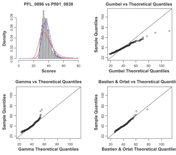
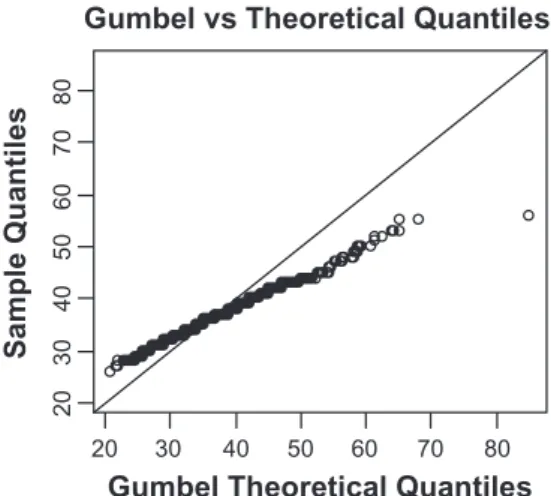
Figure 5. (Top Left) Histogram of the distribution of random scores between the rod shape-determining protein MreB in Pseudomonas fluorescens Pf-5

and the homologous protein in Pseudomonas fluorescens Pf0-1 (Accession numbers PFL_0896 and Pfl01_0838). Only the second sequence was shuffled 1000 times. red curve: gumbel distribution with parameters θ = 33.20788 and β = 7.1206. Blue curve: gamma distribution with parameters δ = 45.1806 and ω = 0.825974. Purple curve: our model with parameters α = 0.001707993, ζ = 26.95872 and η = 1.908571. (top-right) Quantile-quantile plot of

the gumbel theoretical quantile versus the data quantile. (down-left) the gamma theoretical quantile versus the data quantile. (down-right) our model

(11)

Disclosure

This manuscript has been read and approved by all authors. This paper is unique and is not under consid-eration by any other publication and has not been pub-lished elsewhere. The authors and peer reviewers of this paper report no conflicts of interest. The authors confirm that they have permission to reproduce any copyrighted material.

References

1. Altschul SF, Gish W, Miller W, Myers EW, Lipman DJ. Basic local alignment search tool. J Mol Biol. 1990;215:403–10.

2. Altschul SF, Madden TL, Schaer AA, et al. Gapped BLAST and PSI-BLAST: a new generation of protein database search programs. Nucl Acid Res. 1997;25(17):3389.

3. Smith TF, Waterman MS. Identification of common molecular subse-quences. J Mol Biol. 1981;147:195–7.

4. Dayhoff MO, Schwartz RM, Orcutt BC. A model of evolutionary change in proteins. Atlas Prot Seq Struct. 1978;5:345–52.

5. Henikoff S, Henikoff JG. Amino acid substitution matrices from protein blocks. Proc Natl Acad Sci U S A. 1992;89:10915–9.

6. Bastien O, Roy S, Marechal E. Construction of non-symmetric substitu-tion matrices derived from proteomes with biased amino acid distribusubstitu-tions.

C R Biol. 2005;328(5):445–53.

7. Bastien O, Ortet P, Roy S, Maréchal E. A configuration space of homologous proteins conserving mutual information and allowing a phylogeny inference based on pair-wise Z-score probabilities. BMC Bioinformatics. 2005;6:49. 8. Altschul SF. Amino acid substitution matrices from an information theoretic

perspective. J Mol Biol. 1991;219(3):555–65.

9. Mitrophanov AY, Borodovsky M. Statistical significance in biological sequence analysis. Brief Bioinformatics. 2006;7(1):2–24.

10. Karlin S, Altschul SF. Methods for assessing the statistical significance of molecular sequence features by using general scoring schemes. Proc Natl

Acad Sci U S A. 1990;87:2264–8.

PFL_5654 vs Pfl01_5140

Scores

Density

Sample Quantile

s

Sample Quantiles 0 0.00 0.02 0.04 0.06 0.08 0.10 20 40 60 80 30 20 40 50 60 70 20 30 40 50 60 70 20 40 30 60 50 70 20 40 30 60 50 70 20 40 30 60 50 70 30 20 40 50 60 70

Figure 6. (Top Left) Histogram of the distribution of random scores between a hypothetical protein in Pseudomonas fluorescens Pf-5 and the

homolo-gous protein of Pseudomonas fluorescens Pf0-1 (Accession numbers PFL_5654 and Pfl01_5140). Only the second sequence was shuffled 1000 times. red curve: gumbel distribution with parameters θ = 32.25266 and β = 5.941174. Blue curve: gamma distribution with parameters δ = 59.33383 and ω = 0.601377. Purple curve: our model with parameters α = 0.0001799611, ζ = 25.5 and η = 2.5. (top-right) Quantile-quantile plot of the gumbel theoreti-cal quantile versus the data quantile. (down-left) the gamma theoretical quantile versus the data quantile. (down-right) our model theoretical quantile

(12)

11. Altschul SF, Bundschuh R, Olsen R, Hwa T. The estimation of statistical parameters for local alignment score distributions. Nucl Acid Res. 2001;29: 351–61.

12. Pearson WR. Empirical statistical estimates for sequence similarity searches.

J Mol Biol. 1998;276:71–84.

13. Eddy SR. A probabilistic model of local sequence alignment that simpli-fies statistical significance estimation. PLoS Comput Biol. 2008;4(5): e1000069.

14. Poleksic A. Island method for estimating the statistical significance of pro-file-profile alignment scores. BMC Bioinformatics. 2009;10:112.

15. Pang H, Tang J, Chen SS, Tao S. Statistical distributions of optimal global alignment scores of random protein sequences. BMC Bioinformatics. 2005;6:257.

16. Webber C, Barton GJ. Estimation of P-values for global alignments of pro-tein sequences. Bioinformatics. 2001;17:1158–67.

17. Comet JP, Aude JC, Glemet E, et al. Significance of Z-value statistics of Smith—Waterman scores for protein alignments. Comput Chem. 1999;23: 317–31.

18. Bastien O. A Simple Derivation of the Distribution of Pairwise Local Pro-tein Sequence Alignment Scores. Evolutionary Bioinformatics. 2008;4:41. 19. Bastien O, Maréchal E. Evolution of biological sequences implies an

extreme value distribution of type I for both global and local pairwise align-ment scores. BMC Bioinformatics. 2008;9:332.

20. Salemi M, Vandamme AM. The Phylogenetic Handbook: A

Practi-cal Approach to DNA and Protein Phylogeny. Cambridge: Cambridge

University Press; 2003.

21. http://mathworld.wolfram.com/PolyasRandomWalkConstants.html 22. Finch SR. Mathematical Constants. Cambridge: Cambridge University

Press; 2003.

23. Alonso M, Finn EJ. Physics. Reading Massachusetts: Addison-Wesley; 1992.

24. Cohen-Tannoudji C, Diu B, Laloë F. Mécanique quantique I. Paris: Hermann; 1997.

25. Teschl G. Quantum Mechanics and Applications to Schrödinger Operators. Rhode Island: American Mathematical Society; 2009.

26. http://expasy.org/sprot/

27. Fitch WM. Random sequences. J Mol Biol. 1983;163(2):171–6.

28. Huang X, Miller W. A Time-Efficient, Linear-Space Local Similarity Algorithm. Advances in Applied Mathematics. 1991;12:337–57.

29. Ihaka R, Gentleman RR. A language for data analysis and graphics. J Comput

Graph Stat. 1996;5:299–314.

30. Fourdrinier D. Statistique Inférentielle. Paris: Dunod; 2002.

31. Waterman MS, Vingron M. Rapid and accurate estimates of statistical significance for sequence data base searches. Proc Natl Acad Sci U S A. 1994;91(11):4625.

32. Bundschuh R. Rapid significance estimation in local sequence alignment with gaps. J Comput Biol. 2002;9(2):243–60.

33. Chia N, Bundschuh R. Research in Computational Molecular Biology. Berlin: Springer; 2005.

34. Newberg LA. Significance of gapped sequence alignments. J Comput Biol. 2008;15(9):1187–94.

35. Schaffer AA, Aravind L, Madden TL, et al. Improving the accuracy of PSI-BLAST protein database searches with composition-based statistics and other refinements. Nucl Acid Res. 2001;29(14):2994–3005.

36. Agrawal A, Brendel VP, Huang X. Pairwise statistical significance and empirical determination of effective gap opening penalties for protein local sequence alignment. Int J Comput Biol Drug Design. 2008;1(4):347–67. 37. Agrawal A, Huang X. Pairwise statistical significance of local sequence

alignment using multiple parameter sets and empirical justification of parameter set change penalty. BMC Bioinformatics. 2009;10(3):S1. 38. Grishin NV. Estimation of the number of amino acid substitutions per site when

(13)

supplementary Materials

dbasto2<-function(x,alpha = 0.2,xmin = 0) { #heaviside(x,(alpha*pi/2)*exp(-alpha*(x-xmin))*sin(pi*exp(-alpha* (x-xmin))),xmin) heaviside(x,(2*alpha*pi/2)*(x^(2–1))*exp(-alpha*(x^(2)-xmin^(2)))*sin(pi*exp(-alpha*(x^(2)-xmin^(2)))),xmin) } rbasto2<-function(n,alpha = 0.2,xmin = 0) { Z<-runif(n,min = 0,max = 1); (-(1/alpha)*log((1/pi)*acos((2*Z)-1))+xmin^(2))^(1/2) }

#log maximum likehood for the generalized basto distribution #vector of parameters which is c(alpha,xmin)

mlbasto2<-function(para,TT) { alpha<-para[1]; xmin<-para[2]; LL<-length(TT); -sum(log(dbasto2(TT,alpha,xmin))) }

(17)

Example of the basto.r usage (page 5)

1. Copy the example source code (below) in a file named test_basto.r (ascii format). 2. Verify that the two files test_basto.r and the basto r library, are in the same repertory. 3. Just after, launch the R software and write the command line: >source (“test_basti.r”)

source("basto.r")

XX<-rbastog(1000,0.002,20,2)

hist(XX,nclass = 50,,xlim = c(0,100),freq = FALSE);

test.optim<-nlm(mlbastog,c(0.0001,min(XX)-1,2),XX,print.level = 2); X<-seq(from = 0,to = 80,by = 0.01);

funcTest<-dbastog(X,test.optim$estimate[1],test.optim$estimate[2],test. optim$estimate[3]);

lines(X,funcTest,type = "l",col = "blue") X11()

YY<-rbastog(100, test.optim$estimate[1],test.optim$estimate[2],test. optim$estimate[3]);

minG<-min(c(XX,YY)); maxG<-max(c(XX,YY));

qqplot(XX,YY,xlab = "Theoretical Quantiles", ylab = "Sample Quantiles", xlim = c(minG,maxG),ylim = c(minG,maxG))

(18)

qqplot for Gumbel vs Theoretical Quantiles

qqplot for Gamma vs Theoretical Quantiles

qqplot for Bastien & Ortet vs Theoretical Quantiles

qqplot for Bastien & Ortet vs Gumbel

Bastien & Ortet

Gumbel 20 20 30 30 40 40 50 50 60 60 70 20 30 40 50 60 70 80 70 80 20 30 40 50 60 70 80 20 30 40 50 60 70 80 80 20 30 40 50 60 70 80 20 30 40 50 60 70 80 20 30 40 50 60 70 80

Figure s2. Quantile-quantile plot of (top-left) the gumbel theoretical quantile versus the data quantile. (top-right) the gamma theoretical quantile versus

the data quantile. (down-left) our model theoretical quantile versus the data quantile. (top-left) our model theoretical quantile versus the gumbel

theoreti-cal quantile.

PFL_0091 versus Pfl01_0046 with 1000 randomisations

Scores 0 0.00 0.02 0.04 0.06 0.08 0.10 20 40 60 80 Density

Figure s1. Histogram of the distribution of random scores between the Response Regulator NtrC family proteins in Pseudomonas fluorescens Pf-5 and

homologous proteins in Pseudomonas fluorescens Pf0-1 (Accession numbers PFL_0091 and Pfl01_0046). Only the second sequence was shuffled 1000 times. red curve: gumbel distribution with parameters θ = 33.27876 and β = 6.523116. Blue curve: gamma distribution with parameters δ = 53.04861 and ω = 0.6983029. Purple curve: our model with parameters α = 0.001281286, ζ = 27.500000244 and η = 2.

(19)

PFL_4451 vs Pfl01_4222

Scores

Density

Sample Quantile

s

Sample Quantile s 0 0.00 0.02 0.04 0.06 0.08 20 40 60 80 40 60 80 100 40 60 80 100 40 60 80 100 40 60 80 100 40 60 80 100 40 60 80 100

Figure s3. (Top Left) histogram of the distribution of random scores between the two-component system, narL family, sensor histidine kinase in

Pseudomo-nas fluorescens Pf-5 and homologous proteins in PseudomoPseudomo-nas fluorescens Pf0-1 (Accession numbers PFL_4451 and Pfl01_4222). Only the second sequence was shuffled 1000 times. Red curve: Gumbel distribution with parameters θ = 41.79989 and β = 7.047815. Blue curve: gamma stribution with parameters δ = 69.67213 and ω = 0.6583407. Purple curve: our model with parameters α = 8.094621e-04, ζ = 33.5 and η = 2. (top-right) Quantile-quantile

plot of the gumbel theoretical quantile versus the data quantile. (down-left) the gamma theoretical quantile versus the data quantile. (down-right) our

(20)

PFL_0896 vs Pfl01_0838

Scores

Density

Sample Quantile

s

Sample Quantile s 0 0.00 0.02 0.04 0.06 0.08 20 40 60 80 20 40 60 80 100 40 20 60 80 100 40 20 60 80 100 40 20 60 80 100 40 20 60 80 100 40 20 60 80 100

Figure s4. (Top Left) Histogram of the distribution of random scores between the rod shape-determining protein MreB in Pseudomonas fluorescens Pf-5

and the homologous protein in Pseudomonas fluorescens Pf0-1 (Accession numbers PFL_0896 and Pfl01_0838). Only the second sequence was shuffled 1000 times. red curve: gumbel distribution with parameters θ = 33.20788 and β = 7.1206. Blue curve: gamma distribution with parameters δ = 45.1806 and ω = 0.825974. Purple curve: our model with parameters α = 0.001140583, ζ = 26.5 and η = 2. (top-right) Quantile-quantile plot of the gumbel

theo-retical quantile versus the data quantile. (down-left) the gamma theoretical quantile versus the data quantile. (down-right) our model theoretical quantile

(21)

PFL_5654 vs Pfl01_5140

Scores

Density

S am p le Q u an ti le s

Sample Quantile s 0 0.00 0.04 0.08 20 40 60 80 20 30 40 50 60 70 80 30 40 20 50 60 70 80 30 40 20 50 60 70 80 40 30 20 60 50 80 70 40 30 20 60 50 80 70 40 30 20 60 50 80 70

Figure s5. (Top Left) Histogram of the distribution of random scores between a hypothetical protein in Pseudomonas fluorescens Pf-5 and the

homolo-gous protein of Pseudomonas fluorescens Pf0-1 (Accession numbers PFL_5654 and Pfl01_5140). Only the second sequence was shuffled 1000 times. red curve: gumbel distribution with parameters θ = 32.25266 and β = 5.941174. Blue curve: gamma distribution with parameters δ = 59.33383 and ω = 0.601377. Purple curve: our model with parameters α = 0.001270900, ζ = 25.5 and η = 2. (top-right) Quantile-quantile plot of the gumbel theoretical quantile versus the data quantile. (down-left) the gamma theoretical quantile versus the data quantile. (down-right) our model theoretical quantile versus

(22)

PFL_0091_Pfl01_5140_pam70_8_2

Scores

Density

Sample Quantiles 0 0.00 0.10 0.20 20 40 60 80 30 40 50 60 70 30 40 50 60 70 30 40 50 60 70 40 30 60 50 70 40 30 60 50 70 40 30 60 50 70

Alignment Parameter Influence Study

Comparion of a Pseudomonas fluorescens Pf-5 protein with four others Pseudomonas fluorescens Pf0-1 proteins 1. Liste of proteins Pseudomonas fluorescens Pf-5 PFL_0091 448 aa Vs Pseudomonas fluorescens Pf0-1 Pfl01_0046 448 aa Pseudomonas fluorescens Pf0-1 Pfl01_4222 922 aa Pseudomonas fluorescens Pf0-1 Pfl01_0838 345 aa Pseudomonas fluorescens Pf0-1 Pfl01_5140 423 aa

2. List of substitution matrices and alignment parameters (Gapo: gap open penalty, Gape: gap extension penaty)

substitution matrices First choice of parameters second choice of parameters

Blosum 62 gapo: 11; gape: 1 gapo: 9; gape: 2

Pam 70 gapo: 10; gape: 1 gapo: 8; gape: 2

3. Results

(23)

PFL_0091_Pfl01_5140_pam70_10_1

Scores

Density

Sample Quantiles 0 0.00 0.04 0.08 0.12 20 40 60 80 20 30 40 50 60 70 80 90 20 80 40 60 30 20 40 50 60 70 80 90 20 80 40 60 30 20 40 50 60 70 80 90 20 80 40 60 PFL_0091_Pfl01_5140_blosum62_9_2 Scores Density

Sample Quantiles 0 0.00 0.04 0.08 20 40 60 80 80 40 20 80 60 100 40 20 80 60 100 60 20 40 80 100 60 20 40 80 100 40 20 80 60 100 60 20 40 80 100

(24)

PFL_0091_Pfl01_5140_blosum62_11_1

Scores

Density

Sample Quantiles 0 0.00 0.04 0.08 20 40 60 80 20 30 40 50 60 70 40 20 60 30 40 20 50 60 70 40 20 60 30 40 20 50 60 70 40 20 60 PFL_0091_Pfl01_4222_pam70_8_2 Scores Density

Sample Quantile

s

Sample Quantile s 0 0.00 0.10 20 40 60 80 ₃₀ ₄₀ ₅₀ ₆₀ ₇₀ 30 40 50 60 70 30 40 50 60 70 30 40 50 60 70 30 40 50 60 70 30 40 50 60 70

(25)

PFL_0091_Pfl01_4222_pam70_10_1

Scores

Density

Sample Quantiles 0 0.00 0.04 0.08 20 40 60 80 30 40 50 60 70 80 30 50 70 30 40 50 60 70 80 30 50 70 30 40 50 60 70 80 30 50 70 PFL_0091_Pfl01_4222_blosum62_9_2 Scores Density

Sample Quantiles 0 0.00 0.10 0.20 20 40 60 80 30 40 50 60 70 40 30 50 60 70 40 30 50 60 70 40 30 50 60 70 40 30 50 60 70 40 30 50 60 70

(26)

PFL_0091_Pfl01_4222_blosum62_11_1

Scores

Density

Sample Quantile

s

Sample Quantile s 0 0.00 0.04 0.08 20 40 60 80 30 40 50 60 70 80 30 50 70 30 40 50 60 70 80 30 50 70 30 40 50 60 70 80 30 50 70 PFL_0091_Pfl01_0838_pam70_8_2 Scores Density

Sample Quantiles 0 0.00 0.10 0.20 20 40 60 80 20 20 30 40 50 60 70 80 40 60 80 30 20 40 50 60 70 80 20 40 60 80 30 20 40 50 60 70 80 20 40 60 80

(27)

PFL_0091_Pfl01_0838_pam70_10_1

Scores

Density

Sample Quantile

s

S am p le Q u an ti le s 0 0.00 0.04 0.08 20 40 60 80 20 30 40 50 60 70 20 40 60 30 40 50 60 70 20 20 40 60 30 40 50 60 70 20 20 40 60 PFL_0091_Pfl01_0838_blosum62_9_2 Scores Density

Sample Quantile

s

Sample Quantile s 0 0.00 0.10 0.20 20 40 60 80 20 30 40 50 60 70 30 20 40 50 60 70 30 20 40 50 60 70 30 20 40 50 60 70 30 20 40 50 60 70 30 20 40 50 60 70

(28)

PFL_0091_Pfl01_0838_blosum62_11_1

Scores

Density

Sample Quantile

s

Sample Quantile s 0 0.00 0.10 20 40 60 80 20 30 40 50 60 70 80 20 40 60 80 30 20 40 50 60 70 80 20 40 60 80 30 20 40 50 60 70 80 20 40 60 80 PFL_0091_Pfl01_0046_pam70_8_2 Scores D en si ty

S am p le Q u an ti le s 0 0.00 0.04 0.08 20 40 60 80 30 40 50 60 70 30 40 50 60 70 30 40 50 60 70 30 40 50 60 70 30 40 50 60 70 30 40 50 60 70

(29)

PFL_0091_Pfl01_0046_pam70_10_1

Scores

Density

Sample Quantile

s

Sample Quantile s 0 0.00 0.04 0.08 20 40 60 80 ₂₀ ₃₀ ₄₀ ₅₀ ₆₀ ₇₀ ₈₀ 20 40 60 80 30 20 40 50 60 70 80 20 40 60 80 30 20 40 50 60 70 80 20 40 60 80 PFL_0091_Pfl01_0046_blosum62_9_2 Scores Density

Sample Quantile

s

Sample Quantile s 0 0.00 0.10 0.20 20 40 60 80 20 30 40 50 60 70 80 20 40 60 80 30 20 40 50 60 70 80 20 40 60 80 30 20 40 50 60 70 80 20 40 60 80

(30)

publish with Libertas Academica and every scientist working in your field can

read your article

“I would like to say that this is the most author-friendly editing process I have experienced in over 150

publications. Thank you most sincerely.” “The communication between your staff and me has

been terrific. Whenever progress is made with the manuscript, I receive notice. Quite honestly, I’ve

never had such complete communication with a journal.”

“LA is different, and hopefully represents a kind of scientific publication machinery that removes the

hurdles from free flow of scientific thought.” Your paper will be:

• Available to your entire community free of charge

• Fairly and quickly peer reviewed • Yours! You retain copyright

http://www.la-press.com PFL_0091_Pfl01_0046_blosum62_11_1 Scores Density 0 20 40 60 80 0. 00 20 30 40 50 60 70 80 90 Gumbel vs Theoretical Quantiles

Sample Quantile

s

20 30 40 50 60 70 80 90 Gamma vs Theoretical Quantiles

20 30 40 50 60 70 80 90 Bastien & Ortet vs Theoretical Quantiles

Sample Quantile s 0. 08 0. 04 20 60 80 40 20 60 80 40 20 60 80 40