HAL Id: halshs-00850014
https://halshs.archives-ouvertes.fr/halshs-00850014
Preprint submitted on 5 Aug 2013HAL is a multi-disciplinary open access archive for the deposit and dissemination of sci-entific research documents, whether they are pub-lished or not. The documents may come from teaching and research institutions in France or abroad, or from public or private research centers.
L’archive ouverte pluridisciplinaire HAL, est destinée au dépôt et à la diffusion de documents scientifiques de niveau recherche, publiés ou non, émanant des établissements d’enseignement et de recherche français ou étrangers, des laboratoires publics ou privés.
Inequality and bi-polarization in socioeconomic status
and health: Ordinal approaches
Bénédicte H. Apouey, Jacques Silber
To cite this version:
Bénédicte H. Apouey, Jacques Silber. Inequality and bi-polarization in socioeconomic status and health: Ordinal approaches. 2013. �halshs-00850014�
WORKING PAPER N° 2013 – 30
Inequality and bi-polarization in socioeconomic status and health:
Ordinal approaches
Bénédicte Apouey
Jacques Silber
JEL Codes: I1, I3
Keywords: Inequality; Bi-polarization; Ordinal variables; Self-assessed health
P
ARIS-
JOURDANS
CIENCESE
CONOMIQUES48, BD JOURDAN – E.N.S. – 75014 PARIS TÉL. : 33(0) 1 43 13 63 00 – FAX : 33 (0) 1 43 13 63 10
www.pse.ens.fr
CENTRE NATIONAL DE LA RECHERCHE SCIENTIFIQUE – ECOLE DES HAUTES ETUDES EN SCIENCES SOCIALES
1
Inequality and bi-polarization
in socioeconomic status and health:
Ordinal approaches
Bénédicte Apouey* and Jacques Silber** July 15, 2013
Forthcoming in:
Research on Economic Inequality volume 21: Health and Inequality, edited by Pedro Rosa Dias and Owen O’Donnell, Emerald Publishing.
*
Paris School of Economics - CNRS, 48 Boulevard Jourdan, 75014 Paris, France. E-mail: benedicte.apouey@ens.fr
**
Department of Economics, Bar-Ilan University, 52900 Ramat-Gan, Israel, and Senior Research Fellow, CEPS/INSTEAD, Esch-sur-Alzette, Luxembourg.
E-mail: jsilber_2000@yahoo.com
Running head: Bivariate inequality and bi-polarization in income and health
Abstract
Traditional indices of bi-dimensional inequality and polarization were developed for cardinal variables and cannot be used to quantify dispersion in ordinal measures of socioeconomic status and health. This paper develops two approaches to the measurement of inequality and bi-polarization using only ordinal information. An empirical illustration is given for 24 European Union countries in 2004-2006 and 2011. Results suggest that inequalities and bi-polarization in income and health are especially large in Estonia and Portugal, and that inequalities have significantly increased in recent years in Austria, Belgium, Finland, Germany, and the Netherlands, whereas bi-polarization significantly decreased in France, Portugal, and the UK.
Keywords: inequality; bi-polarization; ordinal variables; self-assessed health
2
Introduction
Evaluation of policy reform in the health sector sometimes requires assessment of effects on the dispersion of health - its inequality or polarization - within a population. However, the traditional approach to measuring dispersion requires cardinality of the variable whose dispersion is studied, while the most widely used comprehensive health measure - self-assessed health - is ordinal. This measure is generated by asking respondents to evaluate their health, in general, in response categories ranging from “1: very good” to “5: very poor,” in the World Health Organization recommended version, and from “1: excellent” to “5: poor” in the US version.1 Self-rating has several advantages. First, it offers a summary of an individual’s general state of health. Second, a person’s own appraisal of his or her health is a very good predictor of future mortality and morbidity. The correlation between self-assessed health and mortality remains strong even when controlling for other health variables and for socio-economic status (Idler E. L. & Benyamini Y., 1997).
Because self-assessed health is ordinal rather than cardinal, some dispersion measures, like the Gini coefficient, cannot be applied to it. In a seminal paper, Blair and Lacy (1996) suggested developing specific dispersion measures for ordinal variables, using the cumulative distribution function of the variable of interest. Some studies followed this suggestion and derived uni-dimensional inequality and bi-polarization measures for health (Abul Naga & Yalcin, 2007; Apouey, 2007; Kobus & Miłoś, 2012; Lazar & Silber, 2013).
These univariate measures of dispersion in health alone are arguably less relevant than a bivariate approach that would consider dispersion in a socioeconomic dimension (like income) as well as in health. In this paper, we present indices of inequality and bi-polarization in income and health, which can be used when only ordinal information on individuals’ income and health is available. Typically, income is ordinal when it is given in brackets. The distribution of the exact amount of income between the brackets is unknown and thus it seems natural to assume that the income variable is ordinal.
We develop two approaches to quantify inequality and bi-polarization in income and health. The difference between the two approaches lies in the definition of the absence of inequality and polarization. In the first approach, we make the hypothesis that there is no inequality and
bi-polarization when the actual share of individuals reporting a health category h and an income category y is equal to the product of the marginal shares of individuals in health category h and of individuals in income category y. This approach implies that inequality and bi-polarization will be minimal when health and income are independent. In the second approach, we assume that there is no inequality and bi-polarization when all individuals report the exact same health and income
categories.
3
We provide an empirical illustration of our methods using data on 24 countries from the European Union Statistics on Income and Living Conditions (EU-SILC) for 2004-2006 and 2011. Results suggest that inequalities and bi-polarization are especially large in Estonia and Portugal, and that inequalities have significantly increased in recent years in Austria, Belgium, Finland, Germany, and the Netherlands, whereas bi-polarization significantly decreased in France, Portugal, and the UK. The paper is organized as follows. In the next section we review the existing literature and identify the contribution of our article. We then present the notations and general approach. Subsequent sections develop the two specific approaches to the measurement of inequality and bi-polarization. The penultimate section presents the empirical illustration and the final section makes some concluding remarks.
Previous literature
Dispersion in health when health is a cardinal variable
One approach to quantifying dispersion in self-assessed health consists of two steps. In the first stage, the ordinal self-rated health is transformed into a cardinal variable. Each individual is assigned a cardinal health score depending on his/her answer to the self-assessed health question and his/her observable characteristics (Groot, 2000; Van Doorslaer and Jones, 2003). The underlying assumption is that it is possible to consistently transform the ordinal self-assessed health variable into a cardinal variable. In the second stage, an index of dispersion is computed on the basis of this cardinal health variable.
One strand of this literature quantifies total dispersion in health, irrespective of the socioeconomic characteristics of the individuals (Wolfson & Rowe, 2001). A second strand only looks at a subset of dispersion and quantifies the health dispersion that occurs across the distribution of a socioeconomic variable. Socioeconomic inequality in health is generally assessed using the concentration index (Kakwani, Wagstaff, & Van Doorslaer, 1997; Koolman and Van Doorslaer, 2004; Van Doorslaer and Jones, 2003), whereas social bi-polarization in health can be quantified using the index developed by Apouey (2010).
Dispersion in health when health is an ordinal variable
Allison and Foster (2004) made it clear that the two-step procedure - transforming the ordinal health variable into a cardinal variable and then quantifying health dispersion using a dispersion index for cardinal variables - is fundamentally flawed. Small variations in the scale that is used to transform the ordinal health variable into a cardinal one may reverse the ordering of the distributions that are
4
compared. Allison and Foster (2004) provide an example of a reversal using the variance, whereas Lazar and Silber (2013) provide a second example using the coefficient of variation.
To overcome this limitation, several authors have developed dispersion measures for ordinal health variables that are scale invariant or independent (Abul Naga & Yalcin, 2007; Apouey, 2007; Lazar & Silber, 2013). These authors adopt a univariate approach and quantify overall health dispersion within a population, irrespective of the income levels of the individuals.
The next step is to develop tools to quantify multi-dimensional dispersion in several ordinal variables. This seems critical to describe the evolution of dispersion in the many dimensions of well-being (health, socioeconomic status, life satisfaction, education, among other). The literature on the measurement of bi- or multi-dimensional dispersion for ordinal variables is small. Silber and Yalonetsky (2011) present several measures of multi-dimensional dispersion that can be used when the variable of interest is ordinal and the other variables are nominal/unordered. As far as we know, there is only one paper that examines bi-dimensional inequality in two ordinal variables (Kobus, 2012).
Our approach
Our paper also focuses on the measurement of dispersion in two ordinal variables, namely income and health. Our approach is different from that of Kobus (2012) in two respects. First, our definitions of minimal and maximal dispersion are different. She assumes that dispersion in income and health is minimal when all individuals are in the same income and health category, and that it is maximal when three criteria are met: first, bi-polarization in income is maximal, second, bi-polarization in health is maximal, and third, the medial correlation coefficient between income and health equals 1. In the case where there are three income and health categories, this implies that dispersion is maximal when half of the individuals report the highest health level and the poorest income level, and the other half report the poorest health level and the highest income level. In contrast, in our first approach, we assume that inequality and bi-polarization are minimal when the actual share of individuals reporting a certain combination of income and health levels is equal to the expected share of individuals reporting that combination given the marginal distributions of income and health. In our second approach, we use the same definition of minimal bi-polarization as Kobus (2012), but we consider that bi-polarization in income and health is maximal when half individuals report the lowest income and health levels, whereas the second half report the highest income and health levels. A second difference between our approach and that of Kobus (2012) is that we examine the measurement of both inequality and bi-polarization in ordinal variables, whereas Kobus (2012) focuses on only one type of dispersion measures.
5
Preliminaries
In what follows, we consider two ordinal variable, health and income. We denote H and Y the numbers of health and income categories. Category 1 corresponds to the lowest health and income categories, and categories H and Y to the highest health and income levels. We denote
m
(h
)
and)
( y
m
the median categories of the two variables.We consider a matrix of probabilities p and a matrix of cumulative distribution functions F . p is a
Y
H -dimensional matrix with element
p
h,y indicating the share of the population who reports being in health category h and income category y . By definition, the sum of the elements of matrixp equals 1. .
h
p
denotes the share of the whole population having health level h,p
.y is the share of the population belonging to income class y.y h
F
, is the share of individuals who are in a health category smaller than or equal to h and in an income category smaller than or equal to y :
h i y j j i y hp
F
1 1 , , .Two approaches to measuring bi-dimensional inequality and bi-polarization in income and health
In this subsection, we briefly present our two approaches regarding inequality and bi-polarization in income and health. The goal here is to give some intuition about different ways of conceiving of inequality and bi-polarization in a bi-dimensional context.
The first conception assumes that the marginal distribution of income and health is given, and does not quantify dispersion in these marginal distributions. It also assumes that there is no inequality and bi-polarization if conditional on their income category, individuals have the same probability of reporting a certain health category, and conditional on their health category, individuals have the same probability of reporting a certain income category. The probability matrix for the case of no inequality and bi-polarization corresponds then to the product of the margins
Y H H H Y Yp
p
p
p
p
p
p
p
p
p
p
p
p
p
p
p
p
p
p
. . 2 . . 1 . . . . 2 2 . . 2 1 . . 2 . . 1 2 . . 1 1 . . 1...
...
...
...
...
...
...
6
In our second approach, we quantify overall dispersion in income and health. In contrast with the first approach, we do not assume that the absence of association between income and health means an absence of dispersion. In addition, we consider that there is no inequality and bi-polarization in income and health if there is both perfect equality in income and perfect equality in health. In that case, all individuals report exactly the same income and the same health level. For example:
0
...
0
0
0
0
...
...
...
...
...
...
0
...
0
0
0
0
0
...
0
1
0
0
0
...
0
0
0
0
0
...
0
0
0
0
p
and
1
...
1
1
0
0
...
...
...
...
...
...
1
...
1
1
0
0
1
...
1
1
0
0
0
...
0
0
0
0
0
...
0
0
0
0
F
More generally, the probability matrices with no inequality and bi-polarization contain
)
1
)
((
H
Y
zeros and a single one. In total, there are HY such matrices.Inequality is maximal if all individuals except one are in the lowest health and income cell, whereas one individual is in the highest health and income cell. We suppose that there are n individuals, so the individual in the greatest income and health categories represent a share
n
1
of the population. Then the corresponding matrices for maximal inequality are written as
n
n
p
1
0
...
0
0
0
0
...
0
0
...
...
...
...
...
0
0
...
0
0
0
0
...
0
1
1
and
1
1
1
...
1
1
1
1
1
1
1
1
...
1
1
1
1
...
...
...
...
...
1
1
1
1
...
1
1
1
1
1
1
1
1
...
1
1
1
1
n
n
n
n
n
n
n
n
n
n
n
n
n
n
n
F
This definition is very similar to the definition of maximal inequality in a uni-dimensional context: indeed, uni-dimensional inequality in income is assumed to be maximal when all individuals except one have no income and one individual has all the available income. In the bi-dimensional context, all individuals except one have the poorest health and income status, and one individual has both
excellent health and the highest possible income.
Finally, bi-polarization is maximal if half of the individuals are in the poorest health and income cell, whereas the other half is in the highest health and income cell so that
7
5
.
0
0
...
0
0
0
0
...
0
0
...
...
...
...
...
0
0
...
0
0
0
0
...
0
5
.
0
p
and
1
5
.
0
...
5
.
0
5
.
0
5
.
0
5
.
0
...
5
.
0
5
.
0
...
...
...
...
...
5
.
0
5
.
0
...
5
.
0
5
.
0
5
.
0
5
.
0
...
5
.
0
5
.
0
F
This is similar to the definition of maximal bi-polarization in the univariate context: uni-dimensional bi-polarization in health is maximal if half individuals report the poorest health status whereas the other half reports the highest health status (Apouey, 2007).
General properties of the measures
In what follows, we present the continuity and scale independence properties that are satisfied by our indices.
Property of continuity: The inequality and bi-polarization indices are continuous in p (or F). The property of continuity guarantees that small errors in the values taken by the variables will not lead to big variations in the indices proposed.
Definition of health and income scales: Each health and income category can be attributed a cardinal value according to the scales
s
health
(
s
1health,...,
s
Hhealth)
ands
income
(
s
1income,...,
s
Yincome)
. The scales are arbitrary with the restrictions0
s
1health
...
s
Hhealth and0
s
1income
...
s
Yincome.We denote S the set of scales.
Let D be a bivariate dispersion (i.e. inequality or bi-polarization) index.
Property of scale independence:
D
(
p
1,
s
health1,
s
income1)
D
(
p
1,
s
health2,
s
income2)
(or)
,
,
(
)
,
,
(
F
1s
health1s
income1D
F
1s
health2s
income2D
) for anys
health1,s
health2,s
income1, ands
income2elements of S.
The property means that changing the numerical values of the scales has no influence on the value of the dispersion index.
All the inequality and bi-polarization measures presented in the next two sections satisfy the continuity and the scale independence properties.
8
A first approach to measuring inequality and bi-polarization in income and health: defining conditional indices
Property of minimal inequality and bi-polarization: There is no inequality and bi-polarization if the actual distribution of income and health is identical to the expected distribution (product of the margins).
All the inequality and bi-polarization indices presented in this section satisfy this property, which implies that the measures will be zero if there is no association between income and health.
Measures of inequality
In what follows, we present a theoretical derivation of a number of dispersion indices. A numerical example can be found in Appendix A. We consider the H by Y matrix p of population shares, whose rows and columns correspond respectively to the various health and income categories. Using Theil’s approach to the measurement of inequality, we may derive the following measure of health inequality within income category y:
)]}
/
/(
)
ln[(
)
{(
. , . 1 . h hy y H h h yp
p
p
p
T
(1)where
p
h. is the share in the whole population (whatever the income category is) of individuals having health level h,p
.y the share in the whole population (whatever the health level) of individualsbelonging to income class y, and
p
h,ythe share in the whole population of individuals belonging to income class y and having health level h. The intuitive idea is that a priori the probability for people belonging to income class y of having health level h should be identical to the share in the whole population of individuals with health level h (p
h.). It turns out however that a posteriori this probability is different and equal to(
p
h,y/
p
.y)
.Eq. (1) can then be extended to a measure T of overall inequality in income and health for the whole population: 2
∑
(
)
{(
)
ln[(
.)
/(
,/
.)]}
1 1 . . h hy y Y y H h h yp
p
p
p
p
(2)
It is also possible to measure health inequality on the basis of the Gini index. Here again we first measure health inequality within a given income class by comparing the distribution of the “actual shares”
(
p
h,y)
/(
p
.y)
for each income class y with what could be considered as the “expected shares”2 The Theil index is not defined when some probability
9
. .
/
1
)
(
p
h
p
h. Using the concept of G-matrix3 (Silber, 1989) we then derive the following measure yG
of health inequality within income class y with)...]
[...(
)...]'
)[...(
/
1
(
)..]
/
[...(
)...]'
[...(
h. h,y .y .y h. h,y yp
G
p
p
p
p
G
p
G
(3)where the two vectors (of length H) on both sides of the G-matrix in (3) are ranked by decreasing values of the ratios
(
p
h,y)
/(
p
h.)
.To derive a Gini index
I
G of health inequality for the whole population, we weight the indices given in (3) by the weights of the income classes y. We should however remember that in defining such an overall within groups Gini inequality index, the sum of the weights will not be equal to 1, because each weight will in fact be equal to (p.y)2, in the same way as in the traditional within groups Gini index, the weights are equal to the product of the population and income shares. We therefore end up with)...]
[...(
)...]'
)[...(
/
1
(
)
(
. . , 2 1 . y h h y Y y y Gp
p
p
G
p
I
)...]
[...(
))...]'
)(
[...((
)...]
[...(
)...]'
)[...(
(
1 , . . , 1 . .
Y j y h y h y h Y y h y Gp
p
G
p
p
p
G
p
I
(4)Note that the last expression on the right hand side of (4) shows clearly that one compares “a priori” shares which are equal to the product
((
p
h.)(
p
.y))
of the margins (and hence assumes independencebetween health and income) with “a posteriori” shares
(
p
h,y) which correspond to the actual shares ofcells (h,y) in the total population. It should be stressed here that in computing
I
G we consider first the lowest income class, then the second lowest, etc... since the elements of the row vector))...]'
)(
[...((
p
h.p
.y and of the column vector[...(
p
h, y)...]
on the extreme right of expression (3) areranked by decreasing ratios
(
p
h,y)
/(
p
h.)
, this ranking being implemented separately for each incomeclass y.
We can also compute an expression
)...]
[...(
))...]'
)(
[...((
~
, . . y hy h Gp
p
G
p
I
(5) for the population as a whole, where the elements of the row vector[...((
p
h.)(
p
.y))...]'
and of thecolumn vector
[...(
p
h, y)...]
would have been ranked by decreasing ratios(
p
h, y)
/((
p
h.)(
p
.y))
.To see the difference between the indices
I
Gand I~G the following graphical interpretation is given.10
A graphical illustration of the bivariate approach to health inequality
In Figure 1, we put respectively on the horizontal and vertical axes the cumulative values of the expected shares
(
p
h.)(
p
.y)
and the cumulative value of the actual shares(
p
h, y)
, starting with incomeclass 1 and ranking both sets of shares by increasing ratios
(
p
h,y)
/(
p
h.)(
p
.y)
, that is, by increasingratios
(
p
h,1)
/(
p
h.)(
p
.1)
. Since we start by working only with the individuals belonging to the firstincome class,
p
.1will be common to all these individuals so that the order of ranking of theindividuals will be a function of the ratios
(
p
h,1)
/(
p
h.)
.
Then we do the same for income class 2 andcontinue with the other classes until we end up with income class Y. We obtain a “within income classes inequality curve” (dotted curve in Figure 1) that is made of Y sections, one for each income class. Clearly the slope of this curve is not always non-decreasing. It is non-decreasing within each income class but the curve reaches the diagonal each time we end with an income class.
If now we want to derive the curve that corresponds to expression (5) (dashed curve in Figure 1), we will have to rank both sets of shares (the cumulative shares
(
p
h.)(
p
.y)
on the one hand and thecumulative shares
(
p
h, y)
on the other hand) by increasing values of the ratios(
p
h,y)
/((
p
h.)(
p
.y))
working from the onset with all the H by Y cells (and not, as we did previously, working first with the shares corresponding to the first (poorest) income class and ranking them by increasing ratios
))
)(
/((
)
(
p
h,1p
h.p
.1 and then doing the same successively for all the other income classes.An illustration of the difference between the two approaches is given in Figure 1 where the index
I
Gis equal to twice the area lying between the dotted curve and the diagonal, while the index IG ~
is equal to twice the area lying between the dashed curve and the diagonal. The area lying between these two curves may then be considered as a measure of the degree of overlap between the various income classes in terms of the gaps between the “expected” and “actual” shares.
[Insert Figure 1 here]
Measures of social “pro-poorness” in health
In expression (3) we estimated a within income group y Gini index
G
y which was computed by comparing, for each cell(
h
,
y
)
, its expected share(
p
h.)
in column y with its actual share)
/
(
p
h,yp
.y (see the first expression on the R.H.S. of (3)). This comparison of expected and actual11
index. Moreover the elements of the row vector
[...(
p
h..)..]'
and of the column vector)..]
/
[...(
p
h,yp
.y which appear on the first expression on the R.H.S. of (3) were both classified bydecreasing ratios
(
p
h,y/
p
h.)
.Let us however assume now that, within each income class, we classify these elements (of the vectors
)..]'
[...(
p
h. and[...(
p
h,y/
p
.y)..]
) by decreasing health level h. It can then be shown that what wewould compute would be another kind of relative concentration ratio, one that would measure the link between the ratios
(
p
h,y/
p
.y)
and the health level of the individuals. If these ratios grow in amonotonic way with the level of health then we will get in fact, for each income class, the Gini indices
G
y ratios we previously derived (see expression (3)). The corresponding curve obtained for a given income class by plotting points corresponding on the horizontal axis to the cumulative shares))
)(
((
p
h.p
.y and on the vertical axis to the cumulative shares(
p
h, y)
, both sets of shares beingranked by increasing health level, would be identical to that depicting the inequality measured by
G
y. If however, for a given income class, there is an inverse relationship between the ratios(
p
h,y/
p
.y)
and the level of health of the individuals, the index we propose to compute in this section will be a kind of Pseudo-Gini.4 It will be negative and equal in absolute value to the Gini index measuring the inequality given by
G
y. In such a case the curve will lie above the diagonal (in the range of the corresponding income class) and its slope will be decreasing.5In the more general case we may observe a curve (the solid curve in Figure 1) that can cross one or several times the diagonal but it will still be an increasing curve. If the sum of the areas lying below the diagonal is close to the sum of the areas lying above the diagonal, this Pseudo-Gini will be close to zero. This kind of relative concentration curve was previously suggested to measure the income elasticity of the consumption of a specific good (Kakwani, 1980) and more recently spatial segregation (Dawkins, 2006).
In our case, one may observe that if this curve lies mostly below (resp. above) the diagonal, it means that cases where the actual number of individuals in a given cell is higher than the expected number will be observed mainly among individuals with a high (resp. low) level of health.
The overall measure of “health concentration” in the population, taking such a bivariate approach, would then be equal of the sum of the areas defined for each income class, these areas taking the sign defined previously. If the overall measure of “health concentration” is positive, this would mean that on average it is more common to see a positive link between health and income among richer people than among poorer people. If, however, we find that it is more common to observe an individual with
4
See Silber (1989) for more details on the concept of Pseudo-Gini.
12
a low health level among people with an income lower than the median income and individuals with a high health level among people with an income higher than the median income, then the overall measure of concentration may well be close to zero (despite the fact that we clearly have a positive correlation between income and health). We may therefore want to derive a better measure of such a correlation.
[Insert Figure 1 here]
Measures of bi-polarization
Assume now that the areas defined previously and corresponding to the indices
G
y given in (3) are attributed the following signs. For individuals belonging to an income class which is below the median income, the area will be positive, for a given income class, if it is above the diagonal and negative otherwise, while for individuals belonging to an income class above the median income, the area will be given a positive sign if it is below the diagonal and a negative sign otherwise. The sum of the income class specific areas, assuming the correct sign (as it was just defined) has been attributed to each area, will be a measure of the degree of bi-polarization of the distribution of health.6 It is indeed easy to check that if for income classes below the median income the areas are mostly above the diagonal and for those income classes above the median income, the areas are mostly below the diagonal (the case of the solid curve in Figure 1), we would have here a clear case of bi-polarization, individuals with a high income having usually a high health level and individuals with a low income a low health level. The sum of the areas would then have a positive sign.If, on the contrary, for income classes below the median income, the areas defined previously are mostly below the diagonal while for those income classes above the median income, the areas are mostly above the diagonal, it would mean that individuals with a low income have a high level of health and those with a high income a low health level. The sum of the areas would then be clearly negative, another extreme case of bi-polarization, one corresponding to a negative correlation between health and income.
Finally it is possible that, attributing again to each area the sign defined previously, we end up with a sum of areas whose value would be close to zero. This would indicate that there is no clear correlation between income and health. A zero value for the sum of areas would also be obtained when for each income class the expected number of individuals at each health level is equal to the actual number. This would mean that the conditional probabilities (the probability of having a given health level h, given the income class to which the individual belongs) would be the same whatever the income class - the distributions of health levels would be the same for each income class.
13
A simple numerical illustration of all the concepts which have just been defined is given in Appendix A.
A second approach to measuring inequality and bi-polarization in income and health: overall indices
In this section, we quantify overall bi-polarization in the joint distribution of health and income. This approach differs from that presented in the previous section, because it quantifies the dispersion in the marginal distributions in income and health, and makes a different assumption regarding minimal bi-polarization.
B
(F
)
denotes the overall bi-polarization in health and income associated with the matrix of joint cumulative probabilitiesFProperties
Property of minimal bi-polarization: The bi-polarization index is minimal and equals zero when all individuals report the same income and health category.
Property of maximal bi-polarization: The bi-polarization index is maximum and equals one when half of the individuals report the smallest income and health status whereas the other half of the
individuals report the greatest income and health status.
Definition of a bi-polarization decreasing transfer: Let
p
1 andp
2 be any two matrices (with the same dimensions) representing the probability distributions, and letF
1 andF
2 be the corresponding matrices representing the cumulative distribution functions.F
2 is derived fromF
1 using a bi-polarization decreasing transfer if 1
F
andF
2have the same median health and income categories. In the cells (h,y) for whichh
m
(h
)
andy
m
( y
)
,Fh2,y Fh1,y. In the cells (h,y) for whichh
m
(h
)
andy
m
( y
)
, 1,2
,y hy
h F
F .
For the other cells (h,y),ph2,y p1h,y.
Note that the cells (h,y) for which
h
m
(h
)
andy
m
( y
)
are the cells where both health and income are below the median health and income categories, whereas the cells for whichh
m
(h
)
andy
m
( y
)
are the cells where both health and income are greater than the median health and income categories.14
Property of bi-polarization decreasing transfers: If
F
2 is derived fromF
1 using this type of transfers,F
2 exhibits less bi-polarization thanF
1:B
(
F
2)
B
(
F
1)
.This property implies that overall bi-polarization decreases when a greater proportion of people is concentrated around the median health and income categories, rather than segregated in the two poles of “healthy and wealthy people” (bottom right of the p- and F-matrices) on the one hand and
“unhealthy and poor people” (upper left of the matrices) on the other hand. For instance, let us consider a health variable with five categories and an income variable with five categories as well:
1
.
025
.
1
.
05
.
0
05
.
05
.
05
.
0
05
.
0
05
.
1
.
15
.
05
.
025
.
0
0
05
.
05
.
0
0
0
0
05
.
1p
and
1
825
.
7
.
45
.
2
.
725
.
65
.
55
.
4
.
2
.
525
.
5
.
45
.
35
.
15
.
175
.
15
.
15
.
15
.
1
.
05
.
05
.
05
.
05
.
05
.
1F
The median health category is 3 and the median income category is also 3. We consider a transfer of people from a cell below the medians to another cell below the medians that is “closer” to the
medians: for instance, a transfer of a .05 share of the population from cell (1,1) to cell (2,2). Similarly, we also consider a transfer of people from a cell above the medians to another cell above the medians that is “closer” to the medians: for instance, a transfer of a .025 share of the population from cell (5,4) to cell (4,4). The new matrices are as follows:
1
.
0
1
.
05
.
0
05
.
075
.
05
.
0
05
.
0
05
.
1
.
15
.
05
.
025
.
0
0
1
.
05
.
0
0
0
0
0
2p
and
1
825
.
7
.
45
.
15
.
75
.
675
.
55
.
4
.
15
.
525
.
5
.
45
.
35
.
1
.
175
.
15
.
15
.
15
.
05
.
0
0
0
0
0
2F
The new distribution of health and income is more concentrated around the median health and income categories. According to the property, bi-polarization for F2 is smaller than bi-polarization for F1.
Measures of overall bi-polarization
We generalize the existing measures of bi-polarization for ordinal data in the uni-dimensional approach to the bi-dimensional perspective.
First, we extend the univariate measure of Abul Naga and Yalcin (2007), Apouey (2007), and Reardon (2009) to the bivariate case. Our overall index is a function of the absolute distance between the observed cumulative probabilitiesF , whose elements are
F
h,y, and the maximal bi-polarization F-matrix, whose elements equal 0.5:15
1
1
)
|
5
.
0
|
2
(
1
1 1 , 1
HY
F
B
H h Y y y hSecond, we consider an extension to the bivariate case of an index proposed by Reardon (2009):
H h Y y y h y hF
F
HY
B
1 1 , , 24
(
1
)
1
1
It is easy to prove that the overall bi-polarization indices and satisfy the continuity, scale independence, minimal bi-polarization, maximal bi-polarization, and bi-polarization decreasing transfer properties.
Empirical illustration
In this section, we provide an empirical illustration of the use of the indices developed above, focusing on dispersion in income and health in 2004-2006 and 2011, in 24 European countries.
Our data come from the EU - Statistics on Income and Living Condition (EU-SILC) surveys, whose summary statistics are available from the Eurostat website.7 The EU-SILC project was launched in 2003 on the basis of a “gentleman’s agreement” in six member states of the European Union, as well as in Norway. The starting date for the EU-SILC instrument (under the framework regulation) was 2004 for the EU-15 (with the exception of Germany, the Netherlands and the United Kingdom, which had derogations until 2005), as well as for Estonia, Norway and Iceland. The 10 new member states with the exception of Estonia started in 2005. Bulgaria started in 2006.
The goal of the surveys is to collect timely and comparable data on income, poverty, social exclusion, and living conditions, across European countries. Each EU-SILC surveys is based on a nationally representative probability sample of the population residing in private households and aged 16 years old or over in the respective target country.
We use countries for which information on health and income is available in 2011. Our analysis sample is thus made of Austria, Belgium, Bulgaria, Cyprus, Denmark, Estonia, Finland, France, Germany, Greece, Hungary, Iceland, Italy, Lithuania, Luxembourg, the Netherlands, Norway, Portugal, Romania, Slovakia, Slovenia, Spain, Sweden, and the UK.
We use data for the years 2004-2006 and 2011, which are respectively the first and the most recently available waves. Focusing on these years enables us to get a precise picture of the recent evolution of
16
dispersion in health and income in Europe. As explained above, the first year of data is either 2004, or 2005, or 2006, depending on countries.
The health variable is ordinal self-reported health with five categories: “very bad,” “bad,” “fair,” “good,” and “very good.” Income is also ordinal, since it is given in quintiles. It is computed on the basis of the total equalized disposable income during the year preceding the interview, i.e. total disposable household income divided by the household equalized size, using the modified OECD equivalence scale. This scale gives a weight of 1.0 to the first adult, 0.5 to any other household member aged 14 and over, and 0.3 to each child below age 14.
Note that this section is intended as merely illustrative, as the underlying income variable is continuous rather than ordinal, and the continuous income measure could be obtained if we were to use the original EU-SILC data instead of the published tables. In addition, our income variable is a particular one – quintiles. Consequently, the sample is evenly distributed across categories of income. This implies that in the second approach, our bi-polarization measures are necessarily bounded away from the minimum and maximum.
An interesting feature of the EU-SILC datasets compared to other datasets that are generally used to study inequalities in Europe (such as SHARE or the ESPS) is that they contain information on Eastern European countries. This enables us to get a global picture of income/health inequalities in Europe.
Figure 2 gives the distribution of self-assessed health in the sample. We observe that for both waves the median health category is “Good” in most countries. However there are some exceptions. First, Greece appears as a healthier country than its neighbours, since for both waves the median health category is “Very good.” In contrast, Lithuania and Portugal systematically report poorer health than the rest of Europe. The median health category of these countries is “Fair” for both waves. Finally, Estonia and Hungary may have experienced an improvement of the general health status of the population, since the median health category increased from “Fair” in 2004-2006 to “Good” in 2011. Some other countries also show some signs of an improvement in health. In particular, this is the case in Germany, Portugal, Sweden, Spain, and the UK, since the proportion of individuals in the two top health categories increased whereas those in the three lowest health categories decreased.
In Bulgaria and France, the shares of individuals in the middle categories (“Fair” and “Good”) increased between 2004-2006 and 2011, whereas the shares of individuals in the extreme categories (“Very bad,” “Bad,” and “Very good”) decreased. This means that there is a decrease in (uni-dimensional) bi-polarization in health over time, since the distribution of health was more concentrated around the median health category in 2011.
17
In what follows, we present two tables giving the indices of the bi-polarization and inequality indices developed in the paper.
To derive the inequality and bi-polarization indices based on the first approach, we build for each country and year two matrices whose rows correspond to health and whose columns correspond to income: the first matrix contains the actual shares, whereas the second matrix contains the expected shares. These matrices enable us to draw the “within income classes inequality curve” and the “distributional change curve” and to compute the indices.
We present in Figure 3 a graphical representation of the “within income classes inequality curve” and of the “distributional change curve” for Estonia in 2011. We focus on that country because it has the largest level of inequality and bi-polarization in our analysis sample, which makes the graphical illustration very clear. The curves include five sections, corresponding to the five income quintiles. Note that the two curves are confounded for the top income quintile. The solid curve lies above the diagonal for low-income groups, whereas it is above the diagonal for high-income groups. This implies that poor people are less healthy than expected, whereas rich people are healthier than expected.
[Insert Figure 3 here]
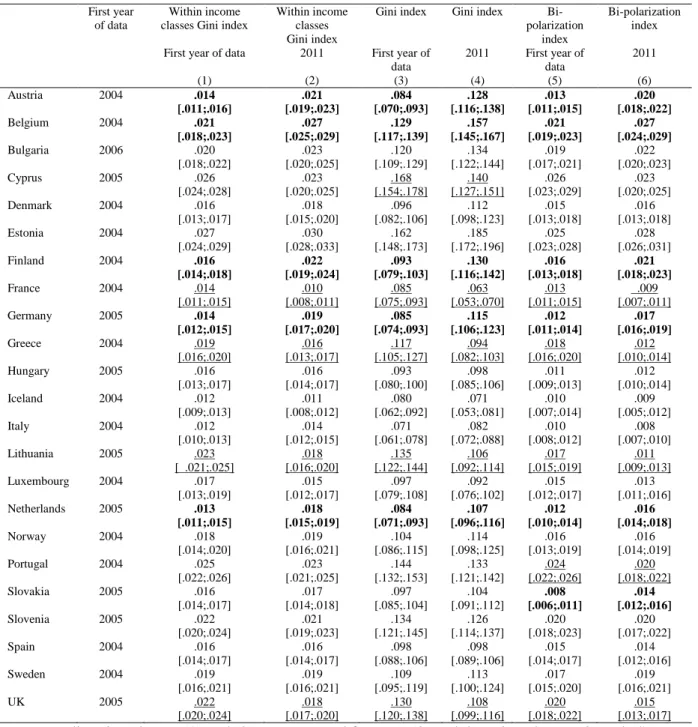
Table 1 contains the inequality and bi-polarization indices derived from the first approach. The technique that we use to compute the confidence intervals for the indices is presented in Appendix B. Inequality and bi-polarization indices are significantly greater than zero in all countries, in both 2004-2006 and 2011.
[Insert Table 1 here]
Our results do not necessarily imply that policies should try to reduce dispersion in health, since not all dispersion can and should be avoided. It would be worth understanding the reasons why dispersion arises in Europe. In particular, future research could investigate a decomposition of the indices by factors, to identify the reasons underlying inequality and bi-polarization. Following the literature on inequality of opportunities in health, these factors could be classified as either circumstances or efforts variables (Rosa Dias, 2009; Trannoy, Tubeuf, Jusot, & Devaux, 2010). If our finding on the positive levels of inequality and bi-polarization reflect differences in circumstances between individuals, this would mean that there are opportunities for reducing inequalities and bi-polarization in health in Europe.
We now turn to the comparison of the levels of dispersion between countries. Note that caution is required when doing this comparison exercise, since differential health reporting might render the
18
indices not comparable between countries (Bago d’Uva, O’Donnell, and Van Doorslaer, 2008). Having this limitation in mind, we rank the countries according to the values of the inequality and bi-polarization indices given in the table. We find that Cyprus, Estonia, and Portugal exhibit a great level of inequality and bi-polarization, in both waves of the data. The very large level of inequality in Estonia in 2004 and 2011 is in line with the substantial level of inequalities in mortality in that country at the end of the 1980s, that was followed by a “tremendous rise of inequalities in mortality” between 1989 and 2000 (Mackenbach, 2006). Our result for Portugal is consistent with the previous literature, that shows that among 13 European countries, Portugal is the most unequal (Van Doorslaer & Koolman, 2004). In contrast, we observe that Iceland and Italy have low levels of health/income dispersion. Our data also suggest that in 2005 the Netherlands had a relatively small level of inequality and bi-polarization, which is consistent with the literature (Van Doorslaer & Koolman, 2004). However, the level of dispersion increased significantly between 2005 and 2011, so that the Netherlands have today a European average level of inequality and bi-polarization.
Looking more closely at the evolution of dispersion over time, we observe that inequality and bi-polarization remained stable in most countries between 2004-2006 and 2011. However, some
countries went through important changes. There is strong evidence that inequality and bi-polarization decreased over time in France, Greece, Lithuania, and the UK. In contrast, inequality and
bi-polarization rose in Austria, Belgium, Finland, Germany, and the Netherlands.
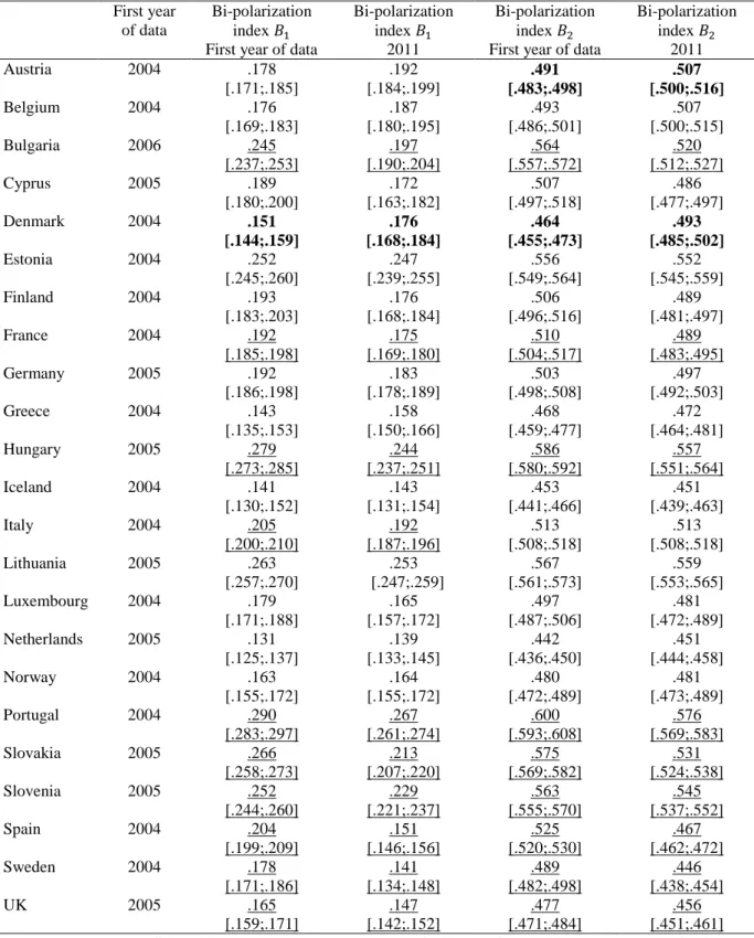
We then turn to the results for our second approach, which is based on a different definition of minimal dispersion. Table 2 contains the bi-polarization indices and for 2004-2006 and 2011.
[Insert Table 2 here]
The table shows a significant level of bi-polarization in all countries both in 2004-2006 and 2011. The two indices indicate that bi-polarization significantly increased in Denmark between 2004 and 2011, whereas it significantly decreased in France, Hungary, Portugal, Slovakia, Slovenia, Spain, Sweden, and the UK. One index also indicates an increase of bi-polarization in Austria and a decrease in Italy.
Comparing the results of Table 2 with the last two columns of Table 1, we find that the evolution of bi-polarization between 2004-2006 and 2011 are often consistent across tables. For instance, both tables show an increase of bi-polarization in Austria and Belgium, and a decrease in Cyprus (these changes can be significant or insignificant). Both tables suggest a significant decrease in bi-polarization in France, Portugal, and the UK between 2004-2005 and 2011.
19
Conclusion
This paper develops original methods to quantify the level of inequality in socioeconomic status and health, when both variables are ordinal. We present two distinct approaches, that are embedded in different definitions of minimal inequality and bi-polarization. The empirical illustration is based on data from the EU-SILC surveys for 24 countries between 2004-2006 and 2011.
Our study suggests several routes for future research. A first avenue could be to provide an axiomatic derivation of bivariate indices, in order to derive the family of dispersion measures that have the most interesting properties. Second, one could develop a decomposition technique for bivariate indices enabling researchers to decompose the total observed income/health disparity into the contribution of several factors. By extension, one could also identify the factors that explain the changes in the level of disparity over time. This is all the more relevant as we find that inequality increased in Austria, Belgium, Finland, Germany, and the Netherlands (see the first four columns of Table 1), and that bi-polarization decreased in France, Portugal, and the UK (see the last two columns of Table 1 and Table 2), over the past decade. A first factor that could explain the rise of inequalities and that could be tested is access to health care services. Indeed, the financial crisis, that started in Europe in 2007, put a strain on health-care systems in some countries. Another relevant factor that could potentially explain the rise in inequality in Germany in particular is the ageing of the population. Indeed, income/health inequality tend to be larger among older generations in that country (Van Kippersluis, Van Ourti, O’Donnell, & Van Doorslaer, 2009).
Acknowledgements: The authors would like to thank Owen O’Donnell for his helpful comments on this article.
20
Appendix A. Numerical example for the first approach to inequality / bi-polarization
Assume two income levels ( and , with the highest income level) and three health levels ( , and , with the highest health level).
Table A1 gives the distribution of the individuals among the six potential cells.
Table A1: Original data
Horizontal margins 50 20 70 20 10 30 30 70 100 Vertical margins 100 100 200
Table A2 gives the actual share of each cell in the total population.
Table A2: Actual shares
Horizontal margins
0.25 0.10 0.35
0.10 0.05 0.15
0.15 0.35 0.50
Vertical margins 0.50 0.50 1 Table A3 gives the expected shares (product of the margins).
Table A3: Expected shares
y=1 y=2 Horizontal margins
0.175 0.175 0.35
0.075 0.075 0.15
0.250 0.25 0.50
Vertical margins 0.50 0.50 1
Finally, Table A4 gives the ratio of the actual over the expected shares and in parenthesis the rank of each cell, as far as this ratio is concerned (cells ranked by increasing values of the ratios).
Table A4: Ratio of actual over expected shares
1.42 (6) 0.57 (1)
1.33 (4) 0.66 (3)
21
Within income classes Gini curve and within income classes Gini index
For the graphical representation we first plot the cumulative values of the expected and actual shares for the lower income class ( ), on the horizontal and vertical axes, these shares being again ranked by increasing values of the corresponding ratios of the actual over the expected shares. Note that when we complete the plot for this lower income class we will have reached the point (0.5;0.5) on the graph. We then do the same thing for the higher income class (y=2) and end up at the point (1;1). This graph then represents the inequality of health opportunity within the income classes.
We can then compute the corresponding within income classes Gini index.
The contribution of the within income class 1 inequality of health opportunities will be written as
and it is easy to find out that
Similarly the contribution of the within income class 2 inequality of health opportunities will be written as
and it is easy to find out that
The overall within income classes inequality of health opportunities is then equal to
Gini curve and the Gini index
Here we draw a graph where on the horizontal axis we plot the cumulative values of the expected shares and on the vertical axis the cumulative values of the actual shares but here all the shares are ranked by increasing ratios of the actual over the expected shares.
We can also compute the corresponding Gini index comparing the expected values (row vector) with the actual values (column vector), the shares in this vector being classified this time by decreasing values (Silber, 1989).
In other words we compute the product e’Ga where e’ is a row vector of the expected shares, a column vector of the actual shares and G is the G-matrix, a matrix whose typical cell is equal to 0
if i=j, to -1 if ji and to +1 if ij. Note again that in both e’ and a all the shares have to be ranked by decreasing values of the ratios of the actual over the expected shares.
In other words we get
It is then easy to find out that
22
Measuring distributional change
But we can also compute an alternative measure. Let us again plot first the cumulative expected and actual shares for the lower income level, but we would rank both sets of cumulative shares by increasing health level. If the higher the actual health level, the higher the ratio of actual over expected shares, then we would get the previous graph.
We could then give an alternative interpretation to this graph and say that it measures the
“distributional change” obtained when comparing actual and expected shares. Since by construction this curve will be completely below the diagonal (and have in fact a non-decreasing slope) we could consider this distributional change as positive since the higher the health level, the higher the ratio of the actual over the expected shares.
If on the contrary, when ranking the cumulative shares, within income class 1, by increasing health level, we find that the lower the health level, the higher the ratio of actual over expected shares, we could consider this distributional change as negative, because, as was just stressed, it indicates that within income class 1, individuals with a low health level are in greater numbers than we would have a priori expected.
Naturally such a distributional curve (for income class 1) can be partly above, partly below the diagonal (especially when we consider more than 3 health levels) and in computing the total distributional change we will have to give a positive sign to any area below the diagonal and a negative sign to any area above the diagonal. However, it turns out that a simple algorithm that takes into account this sign constraint can be implemented to compute the sum of these signed areas. We just have to define a row vector ̃ of the expected shares and a column vector ̃ of the actual shares, both shares being ranked by decreasing health level, and compute the product ̃ ̃ It then turns out that for income level 1
̃ ̃ and it is easy to find that α = ̃ ̃ 0.05125
We can similarly compute the corresponding product ̃ ̃ for income level 2 and find out that ̃ ̃
and it is easy to find that, for income level 2, ̃ ̃ .
The overall distributional change DC will then be expressed as
Measuring bi-polarization
If however our goal is to look at the bi-polarization of the inequality of opportunities, assuming two income levels of equal population size, we should give a positive sign to any area above the diagonal
23
for the lower income level 1 and a positive sign for any area below the diagonal for the higher income class 2, because we would then check whether, among the poor, the lower the health level, the higher the ratio of actual over expected shares and whether, among the rich, on the contrary, the higher the health level, the higher the ratio of actual over expected shares.
In other words a simple measure of bi-polarization B would be written as - and it is then easy to check that in our simple empirical illustration we get
24
Appendix B. Method to compute the confidence intervals
Assume that there are Y income groups and H health levels. Let us call the probability of being in
income category y and of having health level h. The table which was the basis for drawing the distributional change curves is such that
∑ ∑
Let us now define as ( ) with N the number of observations per country.8 Assume
we have a box with N balls of different colors, the number of colors being . In other words, we have balls of color “11,” …, balls of color “hy,” …, and balls of color “HY”.
Let us draw with repetition 1,000 balls from this box and call the number of balls of color “hy”.
Obviously in general is likely to be different from , although it may happen that, for some
“hy”, Call now the ratio . We can use these proportions to
compute the indices originally computed (inequality, distributional change, bi-polarization…).
Let us repeat 500 to 1,000 times this procedure where we draw 1,000 balls with repetition, the number of balls of color “hy” in the box being as before and compute each time the indices of
distributional change, inequality and bi-polarization mentioned previously.
We will then obtain a distribution of each of the indices mentioned previously and can then derive a 5%-95% or a 10%-90% confidence interval for each index. By comparing the confidence interval of an index for a given year with the corresponding confidence interval in another year we can then test whether the index in one year differs significantly from the estimate of the index in another year.
8 We use the minimal number of observations (per country) as a proxy for the number of observations (per country). See the Eurostat website:
http://epp.eurostat.ec.europa.eu/portal/page/portal/income_social_inclusion_living_conditions/documents/tab/Ta b/EU-SILC%20sample%20size.pdf