HAL Id: hal-02176573
https://hal.archives-ouvertes.fr/hal-02176573
Submitted on 8 Jul 2019
HAL is a multi-disciplinary open access
archive for the deposit and dissemination of
sci-entific research documents, whether they are
pub-lished or not. The documents may come from
teaching and research institutions in France or
abroad, or from public or private research centers.
L’archive ouverte pluridisciplinaire HAL, est
destinée au dépôt et à la diffusion de documents
scientifiques de niveau recherche, publiés ou non,
émanant des établissements d’enseignement et de
recherche français ou étrangers, des laboratoires
publics ou privés.
under the Test of Indian Districts. A comparison
Giovanni Fusco, Joan Perez
To cite this version:
Giovanni Fusco, Joan Perez. Bayesian Network Clustering and Self-Organizing Maps under the Test
of Indian Districts. A comparison. Cybergeo : Revue européenne de géographie / European journal
of geography, UMR 8504 Géographie-cités, 2019, �10.4000/cybergeo.31909�. �hal-02176573�
Bayesian Network Clustering and Self-Organizing
Maps under the Test of Indian Districts. A
comparison
Réseaux Bayésiens classificatoires et Self-Organizing Maps à l’épreuve des
districts Indiens. Une comparaison
Giovanni Fusco and Joan Perez
Electronic version URL: http://journals.openedition.org/cybergeo/31909 DOI: 10.4000/cybergeo.31909 ISSN: 1278-3366 Publisher UMR 8504 Géographie-cités
Brought to you by Université Nice Sophia-Antipolis
Electronic reference
Giovanni Fusco and Joan Perez, « Bayesian Network Clustering and Self-Organizing Maps under the Test of Indian Districts. A comparison », Cybergeo : European Journal of Geography [Online], Systems, Modelling, Geostatistics, document 887, Online since 07 March 2019, connection on 08 July 2019. URL : http://journals.openedition.org/cybergeo/31909 ; DOI : 10.4000/cybergeo.31909
This text was automatically generated on 8 July 2019.
La revue Cybergeo est mise à disposition selon les termes de la Licence Creative Commons Attribution - Pas d'Utilisation Commerciale - Pas de Modification 3.0 non transposé.
Bayesian Network Clustering and
Self-Organizing Maps under the
Test of Indian Districts. A
comparison
Réseaux Bayésiens classificatoires et Self-Organizing Maps à l’épreuve des
districts Indiens. Une comparaison
Giovanni Fusco and Joan Perez
Introduction
1 The internal differentiation of a complex, subcontinent-wide geographic space is often
the outcome of a long history associated with more recent fast-evolving processes (metropolization, urban sprawl, polarization, spatial diffusion of innovations, etc.). From this perspective, it should be possible to identify coherent sub-spaces (i.e. spatial structures) inductively from the different features and characteristics of a given geographic space (by gathering information about located items at a finer scale). Inductive reasoning can be used in quantitative geography as a way of discerning patterns and help formulate general laws from the study of specific observations (hypothesis generation). Rather than starting from strong hypotheses ensuing from well-formulated theories, an open and inductive search for common patterns adopts a bottom-up perspective with sub-spaces aggregated a posteriori using model outputs. At the same time, relatively general and even contradictory hypotheses, guiding the feature selection phase of inductive models, can be confronted to the final results (this amounts, in certain respects, to hypothesis testing). Opportunities for this kind of spatial analyses have increased over the past decades with the ever-increasing size of available datasets and computing power (e.g. Batty, 2012). Such an approach usually requires a data-mining phase in order to gather data able to describe the situation of the targeted geographic space in the most exhaustive way with respect to the themes of investigations.
2 Through the case study of urbanization in India, this paper will show the potential (and
the limits) of inductive search of possible regionalizations of a large developing country. More precisely, the main topics of this applied research are urbanization, economic development, consumption levels and sociodemographic modernity in India within the last decade, where these phenomena are analyzed at district level. When compared to countries of old industrialization, India has only recently entered the world economy in a context of strong economic growth and major delay in terms of development (e.g. infrastructures, industrialization, inequalities, etc.). Some authors have rapidly come to the conclusion of a dual India (above all in terms of economic dualism, Gupta and Chakraborty, 2006) giving rise to a spatial dualism (Kurian, 2007, opposes islands of urban, modern and fast developing India to the surrounding rural, poor and critically stagnating countryside), eventually tempered by the existence of transitional spaces.
3 Under strong globalization pressure, India must of course be considered as a fast-evolving
country with historically consolidated spatial inequalities. A rich corpus of research shows the articulation of spatial differences in India, at the district level, with the focus either on demographic indicators (Guilmoto and Rajan, 2013; Durand-Dastès, 2015a) or on poverty, income and socioeconomic development (Banerjee et al., 2015; Durand-Dastès, 2015b; Ohlan, 2013), paying great attention to the social history of India. These questions can be linked to the patterns of urbanization in India, as Cali and Menon (2012) suggest. But the aforementioned works don’t support a simple dual India hypothesis. A much richer multiple India hypothesis seems more appropriate (Durand-Dastès and Mutin, 1995; Cadène, 2008). A large surface area, an old urban structure (dating back to the Aryan Period; e.g. Ramachandran, 1989), unequal stratification of sociocultural factors and an unequal insertion in the world economy (National Research Council, 2010; Mukim and Nunnenkamp, 2012) lead to more possibilities for the arrangement of items over geographic space. It is not our goal to investigate the spatial structures of India at the beginning of the 21st century considering all the facets of its human geography. Denis and
Zérah (2017) highlight the importance of small town dynamics within the Indian urban system while Perez et al. (2018) show through the detection of urban macro-structures that India’s urbanization is underestimated in the official census. It becomes thus interesting to assess the sociodemographic characteristics of Indian districts (household structure, literacy, fertility, absorption of inequalities for the scheduled castes, consumption levels, etc.) in the context of the urbanization process (urban density, insertion in urban macro-structures, etc.), seen as a possible catalyst of sociodemographic modernity and economic development (Cali and Menon, 2012). Indian regions experienced urban transformation following various patterns that defy a singular explanation (e.g. Denis and Marius-Gnanou, 2011; Raman et al., 2015). Even from the specific point of view of our research, the exact geography of the spatial structures of a dual or of a multiple India remain to be ascertained. Is India a mosaic of small subspaces each in different stages (or typologies) of development or are vast regional spaces characterized by given levels of urbanization and socioeconomic development?
4 To test these broad alternative hypotheses on the organization of Indian space and to
formulate new hypotheses on the articulations of spatial structures in India, we thus resorted to AI based algorithms, allowing more freedom in knowledge discovery in databases. A multi-stage clustering of Indian districts has been performed using Bayesian Networks (Perez and Fusco, 2014) and Self-Organizing Maps (Fusco and Perez, 2015). Both approaches have proved to possess a strong capacity to inductively identify the main
spatial structures of the Indian space as well as the ability to deal with incomplete dataset inductively s and with uncertainty issues. These results have been validated internally within each clustering procedure. Since validation between alternative clustering schemes implementing different methodologies and optimizing different quality functions is a difficult task (Haldiki et al., 2001), the aim of this paper is to highlight the similarities between the protocols leading to such remarkable results (statistical parameters, latent factors, etc.) and to evaluate the differences between the segmentation approaches. The need was also felt to compare these relatively new clustering schemes to more traditional multivariate clustering techniques. The aim of the paper is thus mainly methodological, showing how different clustering protocols can converge or diverge in the analysis of a given geographic space. The contribution of the analyses to the understanding of Indian geography deserves its own more specific paper.
5 The paper is organized as follows. The “Theoretical Background, Methodology and Data”
section describes the dataset used in this research and provides an overview of classical multivariate Hierarchical Clustering as well as Bayesian and Artificial Neural Network reasoning when used for clustering spatial units. “Implementing the Clustering Protocols” section details the three protocols developed for this research and highlights their similarities and differences, as well as the validation procedures. “Clustering Results” presents the statistical and geographical results. A final section concludes the paper by discussing the similarities and differences between the clustering protocols and the kind of results they can produce.
Theoretical Background, Methodology and Data
A Database for Inductive Analysis of Indian Space
6 To deal with the complexity of the Indian space, a conceptual model has been developed
(Perez, 2015) to guide the feature selection. 55 spatial indicators were selected to cover six main domains of analysis: economic activity, urban structure, socio-demographic development, consumption levels, infrastructure endowment and basic geographical positioning within the Indian space. All indicators are calculated at the scale of every district of the Indian Union (640 spatial units in 2011) and on a ten-year timeframe whenever possible (2001-2011). Once calculated, the indicators make up a geographic database covering all the Republic of India1 and made of 35200 values. Districts are
practical observing windows for India’s diversity: some are almost completely rural (with practically no urban areas within them), others host several small and mid-sized cities and most of them contain one or two main urban areas organizing a regional urban system. The largest metropolitan areas (namely Delhi, Mumbai and Calcutta) are exceptions as they are subdivided in several districts. Districts are thus convenient spatial units to observe local rural and urban systems in India at a mesoscale. No indicators were used to trace the belonging of districts to the different States of India or to wider cultural or linguistic areas. In this respect, our analysis approach is inductive: we want to cluster Indian districts without any prior assumption of wider subspaces within the Indian subcontinent. However, it should be pointed out that some indicators may slightly assume the existence of spatial structures such as "Distance to Coastline" (which presupposes that the coasts of India are the main interface of the Indian economy with the external world, whereas the Himalayan barrier and the geopolitically tense borders
with Pakistan and Bangladesh do not play the same role), "Distance to tier-1 metropolitan Areas" (which presupposes that the Indian mega-cities polarize at least part of the human activities at a larger scale, as observed everywhere else in the world) and the integration in urban macro-structures (indicators such as "Urban Areas within Extended Urban Area" and "Size Main Extended Urban Area"). The inclusion of a few basic assumptions on the role of geographic space in the organization of India’s diversity is a way to introduce spatial relations in an otherwise a-spatial data-driven approaches. Inductive reasoning is thus somehow coupled with basic theoretically-driven hypotheses, which will in the end be confirmed or infirmed by inductive data-clustering. 5.8% of the 35200 values of the database were missing for different reasons. These missing values have been inferred through a Bayesian statistical procedure2 (4.8% of database). The remaining missing
values (1%) are more a question of non-applicability of indicators and could not be removed (impossibility of calculating ratios related to Scheduled Castes population in districts with no Scheduled Castes).
7 We also stress that the clustering of Indian districts aimed at is not a dual clustering
problem (Lin et al. 2005). The latter imposes proximity constraints both in variable space and in geographic space to cluster similar spatial units in contiguous regions. A SOM implementation of dual clustering has, for example, been proposed by Bação et al. (2004). Using such an approach would amount to assume the homogeneous regionalization hypothesis over the fragmented one, whereas we want to test both hypotheses in our research design.
Clustering using Hierarchical Clustering on Principal Components
8 Hierarchical Clustering can be considered as one of the oldest and easiest methods of
multivariate clustering. It is used to iteratively build a hierarchy of nested clusters, hence its name. Easy to implement, it has been extensively and successfully used in geographical analysis. Hierarchical Clustering can be either a top-down (divisive) or a bottom-up (agglomerative) process. This paper focuses on the latter and most used method in which, in a first stage, given a set of n inputs, each input possesses its own cluster. Then, the pair of clusters that are most similar are combined into a single cluster. Given an appropriate distance measure (Euclidean, Manhattan, Minkowski, etc.), a linkage criterion is used to assess the similarity among clusters (single-linkage, complete-linkage, average-complete-linkage, Ward’s criterion, etc.). Distances are then once again calculated within the new structure obtained and the process is repeated until all the clusters have been gathered together into a single cluster of size n.
9 The cluster hierarchy produced by a Hierarchical Clustering can be visualized through a
hierarchical tree, commonly referred to as a Dendrogram. Using the Dendrogram, the tree can be cut at any level (height) in order to produce the desired number of clusters. As compared to K-means (number of clusters defined a priori), the number of clusters is selected a posteriori. The main advantage of Hierarchical Clustering is that it will always yield the same clustering results as long as the inputs feed the algorithm in the same order, whereas other methods like K-means also perform a random initialization of cluster centers.
10 Multidimensional datasets pose the problem of potentially redundant variables. Principal
component analysis (PCA) is thus commonly used before performing hierarchical clustering. PCA is aimed at reducing the effect of highly correlated variables and can be
considered as a dimension reduction step. PCA allows reducing the dimensional space of the data through an orthogonal transformation retaining a maximized variance per dimension (principal component) in decreasing order. The output can be considered as a new dataset made of linear combinations of the original variables. A Hierarchical Clustering can be applied to this new dataset, resulting in a Hierarchical Clustering on Principal Components (HCPC).
11 A major problem remains in the inability of PCA to deal with missing data and as
discussed previously, India’s dataset contains 1% of those. Most of the time, missing values are imputed (which leads to whole rows ignored in the analysis) or replaced by variable’s means or median in such standard procedures.
Clustering using Bayesian Networks
12 Pearl (1985) coined the term "Bayesian Networks" to describe a method performing
probabilistic Bayesian inference (deriving logical conclusions from known statements and assigning a probability degree to them) between the nodes (representing variables) of a directed acyclic graph (DAG). In practice, Pearl generalized and implemented Bayes' theorem3 to a large number of variables connected within a graph through direct causal
dependencies. The strengths of the dependencies, quantified by conditional probabilities are then used to update the posterior probabilities after incorporation of one or more pieces of evidence, a process called conditioning. The main advantage of Bayesian Networks is that all probabilities are defined on a finite probability space. Thus, it is possible to calculate the joint probability distribution taking into account all the parameters of the model i.e. all the marginal probability distributions (for the independent variables) and all the conditional probability distributions (for the dependent variables). The joint probability distribution of a network is directly related to the structure of the graph since it satisfies the causal Markov condition. On a set of variables x1, x2,…,xn the joint probability distribution is given by:
where ParXi are the parent variables of variable Xi in the network structure.
13 There are several Bayesian Network applications to cluster records (for us spatial units)
into groups. First of all, the structure (i.e. the directed acyclic graph) can be imposed by the modeler or learned from the data. In the first case, only the probabilistic parameters will be learned from data.
14 The most famous pre-imposed network structure for clustering purposes is named Naive
Bayes (Duda and Hart, 1973). It is a star-like structure between all the variable nodes and a newly implemented non-observable node that plays the role of a cluster variable. Oriented arcs are introduced between the cluster variable and each other variable: the cluster variable is supposed to be the latent non-observable cause of all the other variables. In such networks, each particular variable becomes independent of the value of every other variable, once the cluster variable is known, hence its name "naive". Bayesian learning algorithms based on the expectation-maximization (EM) approach can determine the optimal number of clusters and affect a cluster value to each record by maximizing the cluster likelihood, knowing the data.
15 Bayesian structure learning produces more articulated DAGs, and ideally aims at
discovering causal relations among variables (the causal interpretation of probabilistic relations in Bayesian Networks is nevertheless a complex and disputed task), going well beyond clustering purposes. A large number of score-based heuristic algorithms for unsupervised structural learning are commonly used in Bayesian Networks such as Tabu, Maximum Spanning Tree, EQ (learning of Equivalence classes), etc. Perhaps one of the best known is Tabu Search, created by Glover in 1986. Given an optimization problem, Tabu search can be considered as a heuristic algorithm trying to find a suitable solution through a searching and scoring procedure. In more simple terms, Tabu search can be described as a combinatorial optimization algorithm made of the combination of a set of rules and banned solutions. The set of rules is usually composed of a score function and a class of strategies which must be predefined according to the needs. As the iterative process progresses, this method explores the neighborhood of each solution in order to maximize the score function. When a local solution that maximizes the score function is found, during the following iterations, the previous nodes cannot be directly re-selected, hence the name "Tabu": for restricted moves. It therefore forces the algorithm to explore all the possibilities within its neighborhood beyond its local optimum. Bouckaert (1995) adapted this strategy to learn the structure of a Bayesian Network.
16 Unsupervised structure learning can become a preliminary phase of Bayesian clustering
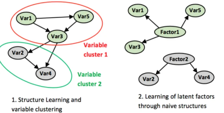
of records in a database. A frequent problem of naive Bayesian classifiers is indeed variable redundancy. When the dimensionality of the problem is particularly high, feature selection alone cannot ensure the absence of groups of redundant variables which would heavily influence the clustering results. The Bayesian network produced through structure learning can then be used to cluster variables (for example through a hierarchical clustering algorithm, HCA) according to the mutual information distance (MacKay 2003) which is encoded in the probabilistic relationships of the model (Heller and Ghahramani, 2005, as applied for example in Fusco, 2016). It thus becomes possible to generate a latent factor by creating a new node for each cluster of variables. In practice, a naive Bayes structure is implemented between each new node and its related variables. The information contained in each cluster of variables is now summarized by a latent factor. In order to perform the final clustering of the records, a new node is once again created and linked to all the latent factors in a naive classifier. The factor values of this ultimate node are the final clustering results. This multi-step clustering procedure is visualized in Figure 1. The final clustering structure can be described as a hierarchical network since the cluster node is connected to all the factors and every factor to its subset of variables.
Figure 1: Combining unsupervised structure learning and naive structures for clustering purposes.
Clustering using Neural Networks (Self-Organizing Maps)
17 Neural Networks are a family of learning models named after their ability to imitate the
biological systems (i.e. the operating way of the human nervous system). The basis of the method amounts to arrange a set of hypothetical neurons so as to form concepts (McCarthy et al., 1955). To reach this objective, Neural Networks learn by being fed with examples as inputs (training data set). The first designed network dates back to the 40s (McCulloch and Pitts, 1943). Yet again, due to processing power limitation, these methods began to be really used only during the 80s. Today, there is a wide range of different kinds of neural networks that are used for different purposes like prediction, pattern learning, clustering, etc. These algorithms make very weak assumptions on the form or distributional properties of interaction data and predictors and can thus be viewed as non-parametric methods (Roy and Thill, 2004).
18 Self-Organizing Maps (SOM) developed by Kohonen (1989) are clustering and pattern
recognition Neural Networks that focus on the topological structure of cluster sets by using a neighborhood function, thus preserving the mutual proximity properties of the input space.
19 SOMs analyze high-dimensional input data (where each record corresponds to an input
vector) by recursively assigning them to a node of a two-dimensional grid. The main advantage of SOM is that it can be considered as an adaptive learning system since its inner parameters change over time. The n x m grid (the map) has a topological structure: each node has a unique (i,j) coordinate and a certain number of direct neighbors (four or six depending on the geometry of the grid: rectangular or hexagonal). Following the equation below, SOM algorithms search the closest map node for each input vector using the square of the minimum Euclidean distance.
Ai,*
weight vector of the current input vector for each map node
d
Euclidean distance from current vector to map node weights.
20 Map nodes are characterized by a weight vector for the different variables of the analysis.
This weight vector evolves during the self-organization process, as input vectors (statistical units) are assigned to the node. Nevertheless, map node weights must be initialized. They can, for example, be set to small standardized values using random initialization. Database records are presented to the SOM in random order. The map node whose weight vector is the closest to a given input vector becomes the best matching unit (BMU) for this record. When the BMU is found, the associated map node gets its weights updated and the input vector under analysis will then be associated with this node. Assigning an input vector to a map node amounts to assigning a record to a cluster. At the difference of K-means, the topological properties of SOMs result in clusters which are organized in terms of reciprocal proximity among them. The specificity of the Self-Organizing Map is that when the BMU is found, a radius parameter will allow the update of the neighboring nodes within this radius. This is particularly useful in order to compare geographic-space proximity and variable-space proximity, as it is often the case in spatial analysis. However, just like K-means, the number of clusters must be specified a
priori.
21 SOM clustering is also confronted to the problem of redundant variables in
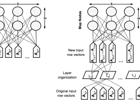
high-dimensional datasets. Wehrens and Buydens (2007) introduced an algorithm that allows using separate layers for different kind of input data: the Super-Organized Map (superSOM). Each layer used in the superSOM algorithm can be seen as a subset of the dataset to be trained. The aim of these subsets is to gather a predefined number of input vectors together in order to reduce the redundant information. In SOM, the input vectors directly feed the map while in superSOM, the elements of the input vectors are first divided between a predetermined numbers of layers before feeding the map. The resulting architectures of SOM and superSOM for clustering purposes are represented in Figure 2. Just like in Bayesian Networks, SuperSOM seems at first glance perfectly suited for processing latent factors, summarizing groups of strongly related variables. Moreover, SuperSOM can process missing and non-applicable values by removing the records before training the Map. They will be mapped later since they are retained in the data (Wehrens and Buydens, 2007).
Figure 2: SOM and superSOM architectures for clustering purposes with a 3x2 grid.
Implementing the Clustering Protocols
Hierarchical Clustering on Principal Component Protocol
R script Presentation and Data Preprocessing22 In order to perform Aggregative Hierarchical Clustering, an R script has been developed
using existing packages (factoextra, FactoMineR, missMDA, fpc)4. Since Hierarchical
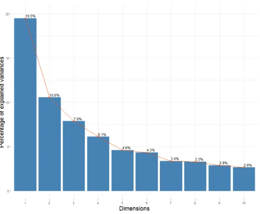
Clustering uses Euclidean distance, values are symmetrized and normalized in order to fully exploit the continuous data of heterogeneous variables. The script loads the necessary packages, imports and preprocesses data (to assure a normal distribution for each variable) and implements functions in order to test for the optimal number of clusters. A Principal Component Analysis is performed and the outputs recorded. Missing data have been replaced by values drawn from a Gaussian distribution according to mean and standard deviation calculated from the other observed values. Variables within this new dataset are no longer correlated and now ordered according to the maximum variance explained from the previous dataset. The first six dimensions account for 53% of the variance of the original dataset. A Hierarchical Clustering of Principal Components (HCPC) can now be carried out.
Figure 3: Scree Plot showing a retained variance of 53% by the first six dimensions.
Aggregative Hierarchical Clustering
23 In hierarchical clustering, distances are used within linkage criteria to aggregate clusters
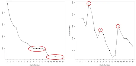
during the iterative merging process. The complete linkage criterion (distance between farthest elements in clusters) has been used since it is known for yielding spherical units (as compared to single link which for example produces chains of clusters). Once the tree is built by the algorithm, the dendrogram can then be cut by the modeler. Since the number of clusters is selected a posteriori in hierarchical clustering, several heuristics and rules-of-thumb can be found to determine the number of clusters. However, it shall be kept in mind that there is no “best solution” as regards to cutting the dendrogram since each partition of the observations corresponds to a differently valid clustering. Amongst the most used heuristics are the Total Within-Cluster Sum of Squares and the Calinski-Harabasz index (Calinski and Calinski-Harabasz, 1974). In the absence of a clear cut-off value, a solution can be to compare the results yielded by different heuristics (as discussed in Zumel and Mount, 2014). The Total Within-Cluster Sum of Squares computes the squared distance of each statistical unit to its cluster center. As a result, it keeps decreasing as the number of cluster increases and becomes smaller. What we are looking on the curve is flat out areas showing the stability of successive clustering results (no drastic change from a dendrogram level to another). Figure 4 identifies two flat out areas from 9 to 14 clusters and from 15 to 20 clusters. The Calinski-Harabasz index is analogous to the F-Ratio in ANOVA and takes into account the number of clusters used, highlighting inflexion points with local maxima. Three of such can be identified in Figure 4: 5, 9 and 15 clusters. Moreover, choosing 9 (synthetic level) and 15 cluster solutions (detailed level) appears to be reasonable since they are supported by the results of the first test. In this
paper, only the synthetic level made of 9 clusters is discussed in the “Clustering Results” section.
Figure 4: Total Within Sum of Squares and Calinski-Harabasz Index on 1 to 20 cluster outputs.
The Bayesian Protocol
Data Preprocessing24 Due to intensive computation, continuous variables are difficult to manage in Bayesian
Networks (probability distributions in BN are multinomial). Variables are thus usually discretized into numerical intervals. The discretization process necessarily produces an information loss, which is the price to pay for efficient Bayesian inference. Since this project’s database is mostly made of continuous variables, the 55 indicators have been discretized into 4 classes using automated k-means algorithms. 5 classes per variable would have led to an overly complex conditional probability table (“Clustering using Bayesian Networks” section) while 3 classes amount to too much information loss. Yet, according to the variable distribution functions, 4 classes were in a few cases not the optimal partition. In those cases, 3 or 5 clusters discretization were applied (Airport Flow, Urban Area Footprint, Density, and University).
Unsupervised Learning of a Bayesian Network
25 The second step is the unsupervised search of probabilistic links among the 55 discretized
indicators. A Tabu Order heuristic algorithm has been executed in order to obtain the initial Bayesian network5. Tabu Order is a specific version of the famous Tabu Search
heuristic algorithm, influenced only by the order thorough which variables feed the network. The most robust arcs of this network have been cross-validated by an arc confidence analysis. The dataset has been randomly divided into 10 subsets (k-fold Jackknife resampling). Given the dataset D and k the number of subsets of D, the Tabu Order algorithm has been executed 10 times for each of the D – Dk sets. The edges found in both 100% of the ten attempts and in the initial network have been extracted and permanently fixed over the network. They represent 35 arcs (60% of the initial network) and can be considered as the most robust arcs of the network. The reverse analysis was
also performed in order to verify if some forgotten arcs appeared in the 10 samplings and not in the initial network, which was not the case. Once the robust arcs are fixed in the network, a further Tabu Search is executed but this time considers the fixed arcs as a constraint. They cannot be removed and the algorithm tries to enrich the network with the strongest probabilistic relationships which do not enter in conflict with the fixed arcs and the DAG assumption. A final network is obtained made up of 55 nodes linked together by 58 arcs.
Variable Clustering
26 The obtained network is then analyzed by a hierarchical clustering algorithm (HCA). The
aim is to detect groups of closely linked variables using the obtained network. However, HCA is a method highly sensitive to random parameters such as the order from which the inputs will feed the algorithm (“Clustering using Bayesian Networks” section). In order to assess the variable clustering, once again the dataset is randomly divided into 10 subsets (k-fold Jackknife resampling) and a HCA is executed each time after removing one of the 10 subsets. Applying ten HCA through a k-fold cross-validation process allows studying the most robust associative patterns among the input variables for each HCA performed. The overall score of the cross-validation for this initial HCA reached 81.44%, but a few variable groupings were particularly unstable (not found within the 10-fold HCA) while others were missing (found within the 10-fold HCA but not within the initial variable clustering). These variable groupings were thus substituted with the more robust groupings produced by the k-fold procedure. The new variable clustering was once again submitted to k-fold cross-validation, showing a much better score of 89.34% and no particularly unstable clusters.
Extraction of Latent Factors
27 Each cluster of variables is subsequently summarized by a latent factor, corresponding to
a more general concept. A naive classifier is built between the individual variables and the non-observable, newly created target node. 17 latent factors plus a single variable, Urban Density (which represents a factor by itself) have been identified (Appendices, Table A.3). 12 of the 18 clusters of variables are particularly robust since clustered together in each of the ten k-folds, as well as on the whole dataset. Latent factors are effective summaries of the information content of the original variables, with an average contingency table fit score of around 80%, as compared to a retained variance of 53% for the standard PCA discussed in the previous section6.
Record Clustering
28 The last step is the creation of an ultimate node, linked to the latent factors through a
naive structure. The segmentation of this factor provides the geographic profiles (clusters of Indian districts). The number of factor values is automatically determined in a random walk exploration of possible clustering schemes. The goal of this exploration is to minimize a score coupling the likelihood function of the factor values knowing the data, and a penalization term for increasing the number of clusters (minimum description length principle), in order to avoid overfitting7. A relative approach to clustering
validation has been implemented in this parameter space, following Halkidi et al. (2001), looking both for stability of clustering solutions and for inflexion points in the internal
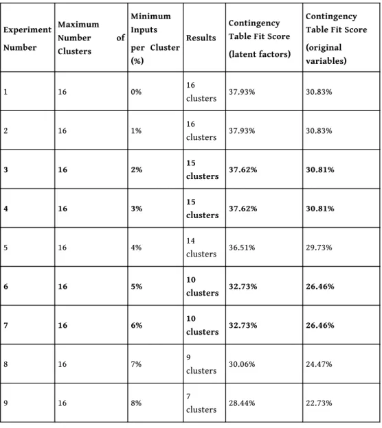
quality parameter (contingency table fit score). This dual validation logic is similar to the one implemented during the HCPC protocol and looks once again for flat out areas and local optima. The maximum number of clusters is set to 16, one cluster more than the upper solution found by the HCPC protocol. Table 1 shows that experiments 1 and 2 reached the upper limit of the maximum number of authorized clusters and experiments 5, 8 and 9 have not been replicated and can thus be considered as more sensitive to parameter variations. The similar contingency fit score between experiments 3 and 4 and experiments 6 and 7 show that in addition to the number of clusters, the input distributions within these clusters are strictly the same. As a result, two robust levels of analysis emerge: Experiment 3-4 which can be considered as a detailed level with 15 clusters and Experiment 6-7; a synthetic level with 10 clusters. Similar results have been obtained with different seeds of the pseudorandom initialization thus showing the robustness of these levels. These two levels are also close to the solutions found in the HCPC protocol. In this paper, only experiment 6-7 (the closest one to the HCPC selected solution) is discussed in the “Clustering Results” section.
Table 1: Results of the Bayesian Experiments for pseudorandom seed 31.
Experiment Number Maximum Number of Clusters Minimum Inputs per Cluster (%) Results Contingency Table Fit Score (latent factors)
Contingency Table Fit Score (original variables) 1 16 0% 16 clusters 37.93% 30.83% 2 16 1% 16 clusters 37.93% 30.83% 3 16 2% 15 clusters 37.62% 30.81% 4 16 3% 15 clusters 37.62% 30.81% 5 16 4% 14 clusters 36.51% 29.73% 6 16 5% 10 clusters 32.73% 26.46% 7 16 6% 10 clusters 32.73% 26.46% 8 16 7% 9 clusters 30.06% 24.47% 9 16 8% 7 clusters 28.44% 22.73%
The SOM/SuperSOM Protocol
R script Presentation and Data Preprocessing
29 In order to automate SOM/superSOM clustering, an R script has been developed using
existing packages (kohonen, class, MASS, dendextend)8. SOMs use mean and variance of
continuous variable values, which presupposes normal, almost-normal or at least symmetric distributions of values. Thus, a symmetrization and normalization of values is also necessary, in order to fully exploit the continuous data of heterogeneous variables. The script loads the necessary packages, imports and preprocesses data, implements automated functions, performs SOM and SuperSOM clustering on both variables and inputs and finally performs a one factor ANOVA to remove non-significant variables. The development of automated functions concerns: the generation of a set of prime number seeds for initialization, the calculation of the Fowlkes-Mallows index associated with each prime seed and the selection of the best initialization.
Variable Clustering
30 Variable grouping in layers within SuperSOM is usually chosen qualitatively prior the
treatment9. In this research, the dataset is first transposed in order to use the variables as
inputs within the SOM function. Since SOM cannot handle missing values, the 1% of input records still presenting missing values are temporarily removed. The output results are a clustering of the original variables thus providing the equivalent of the Bayesian latent factors.
31 The number of clusters has to be decided beforehand in the SOM function and
corresponds to the size of the grid. This will be a crucial point in record clustering (see below) but is of secondary importance in variable clustering, whose goal is just to reorganize variables in order to reduce redundancies in the original database. We thus set the grid size to be as close as possible to the number of clusters obtained by the Bayesian analysis. The SOM grid was set to a 4x4 hexagonal grid in order to cluster the 55 variables into 16 latent factors (Bayesian: 17 latent factors + 1 variable). The original non-transposed dataset is then automatically grouped into a subset of layers according to the clustered variables and the missing values are re-entered since SuperSOM functions are able to handle missing values.
Record Clustering and Variable Removal
32 The layers are weighted according to the number of variables within them and a
superSOM clustering of districts is now carried out, by treating every subset of variables as a distinct layer of spatial information. Yet, an important problem is the number of clusters that should be derived from the data since it shall be chosen a priori for this method. For the previous protocols, relative approaches to clustering validation have helped identify two optimal clustering schemes with 9-10 and 15 clusters, respectively. In SOM/SuperSOM, the number of clusters chosen corresponds to the size of the grid. There are two main ways to obtain clusters in SOM analysis. The simplest solution is to consider the output of the SOM map as the clusters. The second solution is to perform SOM on a large-sized grid and consider the first level of clustering as an intermediate result to be clustered once again. This second level of abstraction is often performed through a
segmentation (partitioning or hierarchical methods) of the U-matrix results (unified distance matrix) which represents the Euclidean distance between the output neurons. Within this research, the simplest solution has been chosen for two reasons (1) Using the knowledge acquired during the HCPC and Bayesian protocols appeared to be a good opportunity to specify the number of clusters. (2) SOM/SuperSOM still require intensive computation. In this protocol they are used 4 times with 20 different pseudo-random seeds (see below). As a result, performing the same analysis on the clustering results than the one applied within the HCPC (Sum of Squares and Calinski-Harabasz Index) protocol would have required running 1600 SOM/SuperSOM.
33 Since the synthetic solution has been chosen for the previous protocols (HCPC: 9 clusters,
BN: 10 clusters), A 3x3 hexagonal grid10 as clustering scheme has been used in order to
later obtain 9 clusters.
34 Lastly, a one factor ANOVA of the clustering results is performed to validate the
SuperSOM clustering and non-significant variables are detected. The non-significant variables are removed11 and the protocol is fully executed once more over the remaining
47 variables (Appendices, Table A.2).
35 It should be pointed out that SOM/SuperSOM applications depend on random
initializations (more precisely pseudorandom initializations generated through a given seed). To address this issue, different clustering solutions were produced with both SOM (variable clustering) and SuperSOM (record clustering) functions for twenty different pseudo-random seeds. The best initialization is automatically retained i.e. the one with the highest Fowlkes-Mallows score. FM index varies between a minimum of 0 (the given clustering differs in every record assignment from the “true” clustering) and a maximum of 1 (the two partitions coincide). In our case no “true” clustering of the data is available, every clustering result, associated with a given random seed is thus compared to every other one. A matrix of FM similarity indexes is then calculated among the clustering results (Fusco and Perez, 2015). The random seed associated to the clustering having the highest FM average yields the most robust initialization of the SOM and SuperSOM algorithms. This step performing robust initialization on both SOM and SuperSOM can be seen as the counterpart of the Bayesian cross-validation process (jackknife k-fold).
Clustering Results
Variables-Space Comparison
36 Clustering results can be compared based on information provided by each individual
indicator within the models (when considering all clusters together). For the Bayesian approach, these indications are given through the amount of mutual information brought by each variable over the ultimate node (geographical cluster of districts). Note that mutual information cannot be added among variables, as different variables can share much of their mutual information with the cluster variable. This information can be replaced by contribution to the inter-class variance of the final clustering for both SOM/ SuperSOM and HCPC models (variance contributions if summed total 100%).
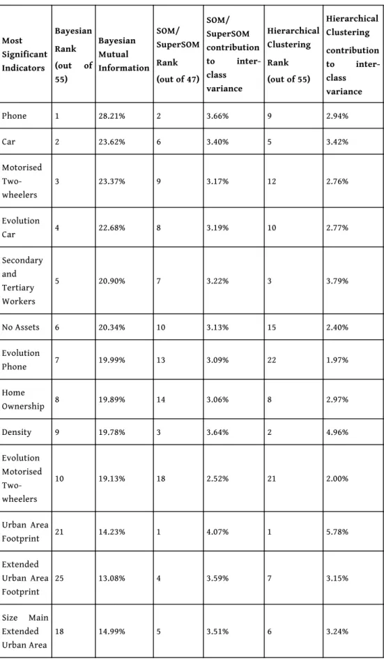
Table 2: Variable contribution to Bayesian, SOM/superSOM and Hierarchical Clustering. Most Significant Indicators Bayesian Rank (out of 55) Bayesian Mutual Information SOM/ SuperSOM Rank (out of 47) SOM/ SuperSOM contribution to inter-class variance Hierarchical Clustering Rank (out of 55) Hierarchical Clustering contribution to inter-class variance Phone 1 28.21% 2 3.66% 9 2.94% Car 2 23.62% 6 3.40% 5 3.42% Motorised Two-wheelers 3 23.37% 9 3.17% 12 2.76% Evolution Car 4 22.68% 8 3.19% 10 2.77% Secondary and Tertiary Workers 5 20.90% 7 3.22% 3 3.79% No Assets 6 20.34% 10 3.13% 15 2.40% Evolution Phone 7 19.99% 13 3.09% 22 1.97% Home Ownership 8 19.89% 14 3.06% 8 2.97% Density 9 19.78% 3 3.64% 2 4.96% Evolution Motorised Two-wheelers 10 19.13% 18 2.52% 21 2.00% Urban Area Footprint 21 14.23% 1 4.07% 1 5.78% Extended Urban Area Footprint 25 13.08% 4 3.59% 7 3.15% Size Main Extended Urban Area 18 14.99% 5 3.51% 6 3.24%
Less Significant Indicators Big Households Evolution 45 7.15% 47 0.39% 52 0.48% Literacy Evolution 32 9.88% 42 0.82% 46 0.75% Banking Evolution 50 5.63% 43 0.80% 35 1.24% Population Evolution for Scheduled Castes 51 5.56% Removed by ANOVA - 54 0.30% Males Ratio Evolution 52 4.99% 44 0.62% 47 0.75% Secondary and Tertiary Workers Evolution 53 4.87% 46 0.53% 48 0.60% SEZ 54 3.66% Removed by ANOVA - 32 1.28% Airport Flows 55 3.35% 45 0.62% 27 1.68%
37 Table 2 shows some similarities among the relative importance of the indicators used to
obtain the clustering of Indian districts12. “Phone” (household mobile phone equipment
rate) has the highest contribution in Bayesian model, the second highest in SOM/ superSOM and is ranked 9th in hierarchical clustering on Principal Components. Other indicators play an important role in the three models especially “Car” (household motorization rate) and its 2001-2011 evolution, “No Assets” (share of households possessing none of the assets listed in Table A.1), “Phone Evolution”, “Motorized two-wheelers” and “Share of Secondary and Tertiary Workers”. Despite the several similarities between these approaches, each model also has its own focuses. One of the main assumptions of this research, stating that the spatial disparities may be studied through the urbanization processes, is not contradicted by these results. Indeed, none of the ad hoc indicators calculated especially for this project are of little significance (this is the case namely for the indicators of urban structure which were not derived from census data). The role of urbanization indicators is more important in SOM/superSOM and HCPC models with top 1 ranking of “Urban Area footprint” and top 2 or 3 of “Density” (several others are among the 10 most important ones). In addition, SOM/superSOM model seems to better take into account the macro-urbanization phenomena (“Extended Urban Area
Footprint” and “Size Main Extended Urban Area”) while HCPC gave more importance to “Secondary and Tertiary Workers”. Other important urbanization indicators of SOM/ superSOM and HCPC models are ranked between 12th and 25th position in Bayesian
clustering. At the same time, the least significant indicators (or indicators removed from the SOM/SuperSOM using ANOVA) are most of the time the same in all methods. Overall socio-demographic evolution indicators are poorly ranked in all methods when compared to socio-economic indicators (especially car, phone, motorized two wheelers). Nonetheless, even if they are not top-ranked, some indicators of socio-demographic evolution receive better consideration within the Bayesian model (e.g. “Literacy Evolution” 32nd in the Bayesian model, 42nd and 46st in SOM/superSOM and HCPC model;
Evolution of Home Ownership, 33rd in Bayesian model but only 41st and 45th in SOM/
superSOM and HCPC model; etc.).
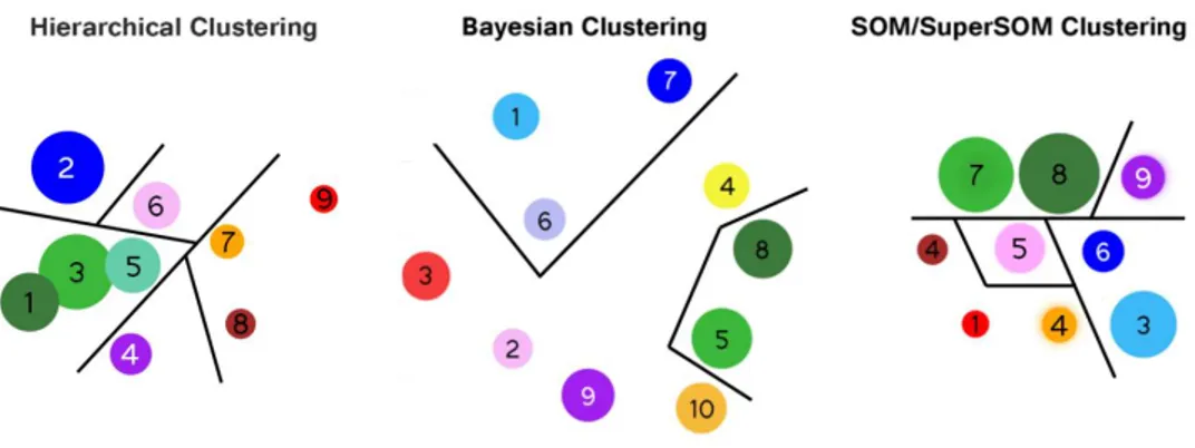
Figure 5: Cluster locations, Neighbourhoods and Sizes in Variable Space.
38 Figure 5 describes the cluster arrangement of the three models. Circle surfaces are
proportional to cluster sizes in terms of number of Indian districts. The arrangement of the HCPC outcome is the projection of the cluster centers in the plane defined by the first two PCA axes. As for Bayesian outcome, it is a 2-dimensional projection of the mutual information distance matrix between the clusters. These two images are of course only a two-dimensional representation and thus not the only possible projection. The figures show that some clusters, and especially cluster 3 (Bayesian) and cluster 9 (HCPC), seem isolated and far away from the other clusters. Some clusters are very close to the point where sometimes a gradient of changing characteristics could be pictured. For those instances, clusters are going to be analyzed together as “families” (line divisions in Figure 5).
39 Cluster locations have a different status in the SOM/SuperSOM analysis. Under the
topological properties of a SOM grid, the centroids that are close to one another have more common features than the centroids that are farther away (right part of Figure 5). Here resides one important difference with the other two representations, which are just projections. Two clusters close to each other in the Bayesian projection could be not so close in the n-dimensional space while for the SOM/superSOM topological structure cluster positions matter much more precisely. From this perspective, cluster 9 for example shares more common features with clusters 6 and 8 than with cluster 3 in the SOM/superSOM topological grid.
Geographic-Space Comparison
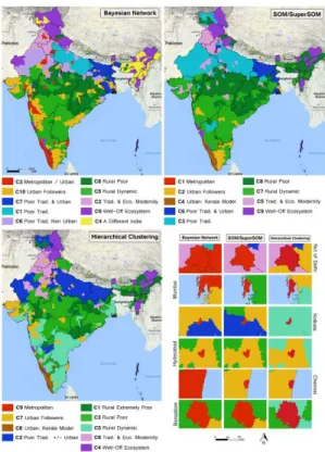
40 The belonging of districts to clusters can be easily projected in geographic space (Figure
6). For practical reasons, specific colors (same as in Figure 5) have been attributed to clusters that correspond in substantial characteristics between the approaches (correspondence between the clustering results are detailed in Appendix A.4). The average values of each indicator, calculated for each cluster (Figure 7), allows the analysis and characterization of the cluster profiles.
Figure 7: Cluster Profiles for Selected Variables.
41 Figure 7 average values are the main results of the SOM/superSOM and HCPC clustering
since these clustering techniques are based on distance maximization among cluster profiles. Bayesian results are based on conditional probabilities over discretized values of the original indicators. Nonetheless, for comparative purposes, the average values of the Bayesian clusters have also been calculated.
42 Profiles are once again regrouped into families. Some clusters are clearly characterized
by a metropolitan/urban habitat, well advanced sociodemographic modernity (important share of “Small Households”, few “Children” per couple, etc.), high standards of living (low “House overcrowding”, higher possession of “Car”, “Phone”, etc.), etc. These profiles (Bayesian C3/C10, SOM/SuperSOM C1/C4/C2, and HCPC C8/C9/C7) are mostly located within Indian metropolitan cities, within districts characterized by a dynamic mid-sized city and within the Kerala state (special cluster for both SOM/SuperSOM and HCPC).
43 The second family (green palette) is characterized by rural districts (C8/C5 Bayesian, C8/
C7 SOM/SuperSOM and C1/C3/C5 HCPC). These clusters encompass vast swaths of the Indian subcontinent mostly located in Madhya Pradesh, Orissa, Jharkhand and Chhattisgarh. Without any surprise, these areas suffer from a lack of basic infrastructures, are always far away from Rank 1 metropolitan areas, urbanization is particularly weak and their populations are associated with socio-economic backwardness (Durand-Dastès 2015b) and low consumption levels. This is particularly the case of clusters C8 (Bayesian, SOM/SuperSOM) and C1 (HCPC). Relatively more dynamic rural clusters can also be identified. C3 in the HCPC model is weakly characterized: though being mainly rural and poor, its average profile is not sharply different from the average of the Indian Republic.
44 The third family (blue palette) is characterized by more traditional sociodemographic
features (C7/C1/C6 Bayesian clustering, C6/C3 in SOM/SuperSOM and C2 HCPC), mainly in northern India. Urbanization patterns are present, especially in Bihar and West Bengal, whose important and dense urbanization falls within larger urban macrostructures. Hierarchical clustering is nevertheless not able to distinguish the differences among the subspaces within this family, grouping them in one cluster only. Sociodemographic tradition (few small households, many big households, important presence of scheduled castes who normally suffer lower living conditions than the general population, many children per couple, high gender disparities) and low living standards are common characteristics of these districts.
45 In addition to these three families, more heterogeneous profiles have also been detected
(C2/C9/C4 Bayesian, C5/C9 SOM/SuperSOM and C6/C4 HCPC). These profiles concern spaces characterized by an intensive farming model (Punjab and Haryana), well-off ecosystems of residential economy associated with tourism (Himalayas) and a subspace far from the typical Indian standards, detected only by the Bayesian approach (C4, "Seven Sisters States": Arunachal Pradesh, Assam, Meghalaya, Manipur, Mizoram, Nagaland and Tripura). This last subspace was assimilated to the more general classes of poor or very poor rural districts by the SOM/SuperSOM and HCPC models.
46 The projected clusters form spatial structures within the Indian subcontinent. However,
if most of these structures are contiguous and relatively compact macro-regions, this is not the case for the most modernized metropolitan profiles (C3 in Bayesian clustering and, even more, C1 and C9 in SOM/SuperSOM and HCPC): highly developed India is an archipelago of disconnected subspaces, often coinciding with the most prominent metropolitan areas.
47 Overall, even if the clustering results are remarkably consistent, noticeable differences
appear and highlight the differences between the aims of the algorithms. The SOM/ SuperSOM and the HCPC algorithms regroup the inputs through a method minimizing the distance between the input vectors. The SuperSOM algorithm can be performed directly on input layers of data. Since this was not possible for hierarchical clustering, this method has been performed on the results of a PCA. Both methods identify clusters which are as homogenous as possible on all the factors of the analysis. Yet, topological properties of neighboring clusters and iterative learning in SOM/SuperSOM enable the constitution of clusters that are statistically far from each other. HCPC, by successive aggregation of most similar clusters leads to clusters closer to the average of the whole dataset. This is well reflected within Figure 7, especially for the traditional and intensive farming model families. Once projected (Figure 6), these clusters are more scattered over the Indian geographic space than their SOM/SuperSOM counterpart.
48 Bayesian networks clustering, on the contrary, focus on the detection of clusters of
districts sharing a few common characteristics using one or several latent factors through a function maximizing the likelihood. Clusters can be relatively heterogeneous on variables which do not contribute to cluster identification. Thus, for example, Bayesian cluster 3 is representative of districts which are precursors in terms of sociodemographic innovation while SOM/SuperSOM cluster 1 and HCPC cluster 9 (strictly similar, Table A.4) are only composed of the major Indian metropolitan areas. The strong common features of several latent factors related to socio-demographic modernity are enough to create a profile for the Bayesian method. Conversely, SOM/SuperSOM algorithms were forced to optimize all the layers of information and were thus not able to ignore the layers that
displayed very strong urban characteristics (Appendices, Table A.2: Layer 4, 7 and 15). The same pattern happened with several other clusters such as with the urban followers composed of dynamic mid-sized cities (Bayesian C8, SOM/SuperSOM C10, HCPC cluster 7), or for the Kerala model (SOM/SuperSOM C4, HCPC cluster 8) that showed strong signs of socio-demographic modernity without possessing the features of heavy urbanized territories. In a similar way, the non-presence of Scheduled Castes within the "Seven Sister States" is a feature strong enough for the Bayesian application to detect a cluster (C4), while the other applications missed this cluster due to their incapacities to build profiles based solely on the characteristics of a few variables/layers. Successive aggregation in HCPC leads to a pattern in which a local optimum for a pre-defined number of clusters is dependent upon the preceding choices of aggregation. As a result, only one cluster emerges for the family of traditional poor districts, making no difference between rural and urban areas, while the other methods detected 2 or 3 clusters, with, in addition to socio-demography, interesting differences in term of urbanization and macro-urbanization. The fact that HCPC is the only method detecting 2 clusters of poor rural India (cluster 1 and 3) could also be considered as a poor performance since the subtle differences between these clusters were not aimed at by our feature selection.
49 Results finally suggest that SOM/superSOM and HCPC models are forced to make a
difference between the two metropolitan clusters of India. Bayesian clustering, by recognizing a few distinguishing metropolitan traits (above all in terms of consumption levels and socioeconomic modernity) overlooks the differences in urbanization patterns. On the same basis, Bayesian clustering recognizes a wider space of urban followers, whenever urbanization patterns, higher consumption levels and some degrees or socioeconomic and demographic modernity meet, without forcing homogeneity on all these factors. Bayesian clustering and HCPC also differentiate apparently homogeneous rural India, even if this was not the goal of our feature selection. Exploring these differences in terms of an attentive reading of Indian geography deserves a more profound analysis, going beyond the scope of this paper.
Discussion and Conclusions
50 Three different clustering techniques have been tested and coupled with step-by-step
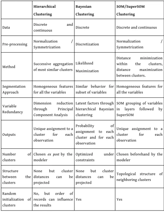
protocols in order to find clusters as robust as possible. Despite the similarities that have been deliberately implemented throughout the protocols (e.g. cross-validation/robust initialization; determination of latent factors / principal components / variable layers), fundamental differences characterize these clustering techniques, as summarized in Table 3.
51 Concerning the clustering results, some clusters are very similar in every approach but
discrepancies between clusters are nonetheless to be found. The major difference, reflected in the output space, lies in the fact that SOM/SuperSOM algorithms regroup the inputs by minimizing intra-class variance and maximizing inter-class variance, Bayesian clustering focuses on common characteristics of a selected number of latent factors and HCPC successively aggregates similar clusters. SOM and HCPC require homogeneous behavior of records over variables which will be clustered together. In the Bayesian approach a subset of data presenting a precise pattern on some variables is enough to identify a latent factor, the remaining data being considered as noise. In this respect, the
Bayesian approach accommodates for more heterogeneity in the statistical population under enquiry.
Table 4: Differences and Similarities between Bayesian and SOM/SuperSOM Clusterings.
Hierarchical Clustering Bayesian Clustering SOM/SuperSOM Clustering
Data Discrete and
continuous Discrete Discrete and continuous
Pre-processing Normalization /
Symmetrization Discretization
Normalization / Symmetrization
Method Successive aggregation of most similar clusters
Likelihood Maximization
Distance minimization within the clusters, distance maximization between clusters.
Segmentation Approach
Homogeneous features for all the variables
Similar behavior for subset of variables
Homogeneous features for all the variables
Variable Redundancy
Dimension reduction through Principal Component Analysis
Latent factors through hierarchical Bayesian clustering
SOM grouping of variables in layers followed by SuperSOM
Outputs
Unique assignment to a cluster for each observation
Probability of assignment to each cluster and for each observation
Unique assignment to a cluster for each observation
Number of clusters
Chosen ex post by the modeler
Optimized under constraints
Chosen beforehand by the modeler
Structure between the clusters
None but cluster distances can be projected
None but cluster distances can be projected Topological structure of neighboring clusters Random initialization of clusters
No, but order of records can influence the results
Yes Yes
52 Since SOM/superSOM and HCPC algorithms are always looking for homogeneous features
within the whole dataset, the choice of indicators to be used as inputs (feature selection) must be wisely and thoughtfully considered. This is especially true in SOM/SuperSOM since each variable or each dimension (layer) possesses the same weight, while working on a PCA matrix allows avoiding this issue when using hierarchical clustering. Therefore, removing non-significant variables through an ANOVA substantially improves the results of a SOM/SuperSOM application. This step is also dispensable in a Bayesian application. Indeed, for each cluster, only relevant information is taken into account by the Bayesian
algorithms. A non-significant factor for the overall model can by very significant for a very specific profile only (e.g. Bayesian Cluster C4 using latent Factor 14).
53 Overall, as the empirical test on the Indian data shows, Bayesian Networks and
Self-Organizing Maps used for clustering purposes are complementary and produce results which are recognized to be just as good, if not better, than more traditional HCPC. HCPC performed on a PCA matrix yields results close to the SOM/SuperSOM application but possesses several drawbacks linked to the absence of a learning phase in the sense of artificial intelligence (this can lead to less robust results and to the trap of local optima). Even if clustering results of all three models indicate a diversity within Indian space which seems to invalidate the hypothesis of a dual India, a more careful evaluation of the geographical results will be left to a future work. The very aim of the paper was to show what remains constant and what changes when precise methodological choices are made. However, we remark that the spatial structures identified within this work also derive from the selected items of research and the available data.
BIBLIOGRAPHY
Bação F., Lobo V., Painho M., 2004, "Geo-Self-Organizing Map (Geo-SOM) for Building and Exploring Homogeneous Regions", in Egenhofer M.J., Freksa C., Miller H.J., (eds.): GIScience, LNCS 3234, Berlin: Springer, 22–37.
Banerjee A. N., Nilanjan B., Jyoti P.M., 2015, The dynamics of income growth and poverty: Evidence from districts in India. Development Policy Review, Vol.33, No.3, 293-312.
Batty M., 2012, "Smart cities, big data", Environment and planning B: Planning & Design, Vol.39, No.2, 191-193.
Bayesia., 2010, BayesiaLab user guide, Laval: Bayesia.
Bouckaert R.R., 1995, Bayesian belief networks: from construction to inference. Thesis, University of Utrecht.
Cadène P., 2008, Atlas de l’Inde, une fulgurante ascension, Paris, Autrement.
Cali M., Menon C., 2012, "Does urbanization affect rural poverty? Evidence from Indian districts",
The World Bank Economic Review, Vol.27, No.2, 171-201.
Calinski T., Harabasz J., 1974, "A dendrite method for cluster analysis", Communications in Statistics . Vol. 3, No. 1, 1-27.
Denis E., Marius-gnanou K., 2010, "Toward a better appraisal of urbanization in India", Cybergeo :
European Journal of Geography [Online], Systèmes, Modélisation, Géostatistiques, document N°569
URL : https://journals.openedition.org/cybergeo/24798
Denis E., Zérah M-H., 2017, Subaltern Urbanisation in India: An Introduction to the Dynamics of
Ordinary Towns, Springer.
Durand-Dastès F., and Mutin G., 1995, Afrique du Nord, Moyen-Orient, Monde Indien, in Brunet, R (eds)., Géographie universelle, Vol. 10, Paris, Belin - Reclus.
Durand-Dastès F., "Les hautes densités démographiques de l’Inde", Géoconfluences [Online], (dossier) Le monde indien : populations et espaces, 24 Mars 2015a, URL : http://
geoconfluences.ens-lyon.fr/informations-scientifiques/dossiers-regionaux/le-monde-indien-populations-et-espaces/articles-scientifiques/les-hautes-densites-demographiques-de-linde Durand-Dastès F., "Backward India" À la recherche de ses caractères et de ses lieux, EchoGéo [Online], Inde : le grand écart spatial, Avril 2015a, URL: http://echogeo.revues.org/14266 Fusco G., 2016, "Beyond the built-up form/mobility relationship: Spatial affordance and lifestyles", Computer Environment and Urban Systems, No.60, 50-66.
Fusco G., Perez, J., "Spatial Analysis of the Indian Subcontinent: The Complexity Investigated through Neural Networks", 14th International Conference on Computers in Urban Planning and Urban
Management [Online], July 2015, Cambridge (Ma.), Proceedings 287, 1-20. URL : http://
web.mit.edu/cron/project/CUPUM2015/proceedings/Content20/ analytics/287_fusco_h.pdf Guilmoto C. Z., Rajan S. I., 2013, "Fertility at the district level in India. Lessons from the 2011 Census", Economic and Political Weekly, Vol. 48, No.23, 59-70.
Haldiki M., Batistakis Y., Vazirgiannis M., 2001, "On Clustering Validation Techniques" Journal of
Intelligent Information Systems, Vol.17, No.2/3, 107-145.
Heller K.A., Ghahramani Z., 2005, "Bayesian Hierarchical Clustering", Proceedings of the 22nd
international conference on Machine learning, 297-304.
Kohonen T., 1989, Self-organizing and associative memory. (3rd ed.), Berlin: Springer.
Kurian N.J., 2007, "Widening economic & social disparities: implications for India", Indian Journal
of Medical Research, Vol.126, No.4, 374-380.
Gupta M.R., Chakraborty B., 2006, "Human Capital Accumulation and Endogenous Growth in a Dual Economy", Hitotsubashi Journal of Economics, Vol. 47, No. 2, 169-195
Lin C.-R., Liu K.-H., Chen M.-S., 2005, "Dual Clustering: Integrating Data Clustering over Optimization and Constraint Domains", IEEE Transactions on Knowledge and Data Engineering, Vol.17, No.5, 628-637.
MacKay D., 2003, Information theory, inference and learning algorithms. Cambridge: Cambridge University Press.
McCarthy J., Minsky M., Rochester N., Shannon C., 1955, A Proposal for the Dartmouth Summer
Research Project on Artificial Intelligence, Hanover (NH).
McCulloch W., Pitts W.H., 1943, "A Logical Calculus of the Ideas Immanent in Nervous Activity",
Bulletin of Mathematical Biophysics, Vol.5, 115-133.
Mukim M., Nunnenkamp P., 2012, "The location choices of foreign investors: A district-level analysis in India", The world economy, Vol.35, No.7, 886-918.
National Research Council., 2010, Understanding the Changing Planet. Strategic Directions for the
Geographical Sciences, Washington: National Academic Press.
Ohlan R., 2013, "Pattern of regional disparities in socio-economic development in India: District level analysis", Social Indicators Research, Vol.114, No.3, 841-873.
Pearl J., 1985, "Bayesian networks: A model of self-activated memory for evidential reasoning",
Perez J., 2015, Spatial Structures in India in the Age of Globalisation. A Data-driven Approach. Thesis, UMR 7300 Espace-CNRS, University of Avignon.
Perez J., Fusco G., 2014, "Inde rurale, Inde urbaine : qualification et quantification de l’aptitude au changement des territoires indiens", in Moriconi-Ebrard F., Chatel C., Bordagi, J. (eds.), At the
Frontiers of Urban Space. Small towns of the world: emergence, growth, economic and social role, territorial integration, governance, Proceedings, Avignon, Publication collective, 316-339.
Perez, J., Fusco, G., Moriconi-Ebrard, F., 2018, "Identification and quantification of urban space in India: Defining urban macro-structures". Urban Studies, Online first, SAGE Publications, 1-17. Ramachandran R., 1989, Urbanization and Urban Systems in India, Oxford University Press. Raman B., Prasad-Aleyamma M., De Bercegol R., Denis E., Zerah M.H., 2015, Selected Readings on
Small Town Dynamics in India, USR 3330 Savoirs et Mondes Indiens, working papers series, No.7,
SUBURBIN Working papers series no. 2.
Roy J.R., Thill J-C., 2004, "Spatial interaction modelling", Papers in Regional Science, Vol.83, No.1, 339-361.
Wehrens R., Buydens L.M.C., 2007, "Self- and Super-organizing Maps in R: The kohonen Package",
Journal of Statistical Software, Vol.21, No.5.
Zumel N., Mount J., 2014, Practical Data Science with R, Manning Publications.
APPENDIXES
Table A.1: List of the 55 Variables used as Inputs for Clustering of Indian Districts
Variable Name Unit Ref.
Year Source
Population Inhabitants 2011 Census of India
Population Evolution (Decadal
Growth Rate) Percentage points
2001
-2011 Census of India
Scheduled Caste (SC) Population Share of Population 2011 Census of India
SC Population Evolution Percentage points 2001
-2011 Census of India
Small Households (HHLDS) (less
than 3 peoples) Share of HHLDS 2011 Census of India
Small HHLDS Evolution Percentage points 2001
-2011 Census of India
Big HHLDS (more than 6 peoples) Share of HHLDS 2011 Census of India
Big HHLDS Evolution Percentage points 2001