HAL Id: hal-02873941
https://hal.archives-ouvertes.fr/hal-02873941
Submitted on 18 Jun 2020
HAL is a multi-disciplinary open access
archive for the deposit and dissemination of
sci-entific research documents, whether they are
pub-lished or not. The documents may come from
teaching and research institutions in France or
abroad, or from public or private research centers.
L’archive ouverte pluridisciplinaire HAL, est
destinée au dépôt et à la diffusion de documents
scientifiques de niveau recherche, publiés ou non,
émanant des établissements d’enseignement et de
recherche français ou étrangers, des laboratoires
publics ou privés.
An AeroCom initial assessment -optical properties in
aerosol component modules of global models
S. Kinne, M Schulz, C. Textor, S. Guibert, Yves Balkanski, S. E. Bauer, T.
Berntsen, T. Berglen, O. Boucher, M. Chin, et al.
To cite this version:
S. Kinne, M Schulz, C. Textor, S. Guibert, Yves Balkanski, et al.. An AeroCom initial
assess-ment -optical properties in aerosol component modules of global models. Atmospheric Chemistry
and Physics, European Geosciences Union, 2006, 6, pp.1815-1834. �10.5194/acp-6-1815-2006�.
�hal-02873941�
© Author(s) 2006. This work is licensed under a Creative Commons License.
Chemistry
and Physics
An AeroCom initial assessment – optical properties in aerosol
component modules of global models
S. Kinne1, M. Schulz2, C. Textor2, S. Guibert2, Y. Balkanski2, S. E. Bauer3, T. Berntsen4, T. F. Berglen4, O. Boucher5,6, M. Chin7, W. Collins8, F. Dentener9, T. Diehl10, R. Easter11, J. Feichter1, D. Fillmore8, S. Ghan11, P. Ginoux12,
S. Gong13, A. Grini4, J. Hendricks14, M. Herzog12, L. Horowitz12, I. Isaksen4, T. Iversen4, A. Kirkev˚ag4, S. Kloster1, D. Koch3, J. E. Kristjansson4, M. Krol16, A. Lauer14, J. F. Lamarque8, G. Lesins17, X. Liu15, U. Lohmann18,
V. Montanaro19, G. Myhre4, J. E. Penner15, G. Pitari19, S. Reddy12, O. Seland4, P. Stier1, T. Takemura20, and X. Tie8 1Max-Planck-Institut f¨ur Meteorologie, Hamburg, Germany
2Laboratoire des Sciences du Climat et de l’environnement, Gif-sur-Yvette, France 3The Earth Institute at Columbia University, New York, NY, USA
4University of Oslo, Department of Geosciences, Oslo, Norway
5Laboratoire d’Optique Atmosph’erique, USTL/CNRS, Villeneuve d’Ascq, France 6Hadley Centre, Met Office, Exeter, UK
7NASA Goddard Space Flight Center, Greenbelt, MD, USA 8NCAR, Boulder, Colorado, USA
9EC, Joint Research Centre, IES, Climate Change Unit, Ispra, Italy
10Goddard Earth Sciences and Technology Center, UMBC, Baltimore, MD, USA 11Batelle, Pacific Northwest National Laboratory, Richland, USA
12NOAA, Geophysical Fluid Dynamics Laboratory, Princeton, NJ, USA 13ARQM Meteorological Service Canada, Toronto, Canada
14DLR, Institut f¨ur Physik der Atmosph¨are, Oberpfaffenhofen, Germany 15University of Michigan, Ann Arbor, MI, USA
16Institute for Marine and Atmospheric Research Utrecht (IMAU) Utrecht, The Netherlands 17Dalhousie University, Halifax, Canada
18ETH Z¨urich, Switzerland
19Universita degli Studi L’Aquila, L’Aquila, Italy 20Kyushu University, Fukuoka, Japan
Received: 25 May 2005 – Published in Atmos. Chem. Phys. Discuss.: 8 September 2005 Revised: 6 February 2006 – Accepted: 13 February 2006 – Published: 29 May 2006
Abstract. The AeroCom exercise diagnoses multi-component aerosol modules in global modeling. In an ini-tial assessment simulated global distributions for mass and mid-visible aerosol optical thickness (aot) were compared among 20 different modules. Model diversity was also ex-plored in the context of previous comparisons. For the com-ponent combined aot general agreement has improved for the annual global mean. At 0.11 to 0.14, simulated aot values are at the lower end of global averages suggested by remote sensing from ground (AERONET ca. 0.135) and space (satel-lite composite ca. 0.15). More detailed comparisons, how-ever, reveal that larger differences in regional distribution and significant differences in compositional mixture remain. Of
Correspondence to: S. Kinne
particular concern are large model diversities for contribu-tions by dust and carbonaceous aerosol, because they lead to significant uncertainty in aerosol absorption (aab). Since aot and aab, both, influence the aerosol impact on the radia-tive energy-balance, the aerosol (direct) forcing uncertainty in modeling is larger than differences in aot might suggest. New diagnostic approaches are proposed to trace model dif-ferences in terms of aerosol processing and transport: These include the prescription of common input (e.g. amount, size and injection of aerosol component emissions) and the use of observational capabilities from ground (e.g. measurements networks) or space (e.g. correlations between aerosol and clouds).
1816 S. Kinne et al.: An AeroCom initial assessment
1 Introduction
Aerosol is one of the key properties in simulations of the Earth’s climate. Model-derived estimates of anthropogenic influences remain highly uncertain (IPCC, Houghton et al., 2001) in large part due to an inadequate representation of aerosol. Aerosol originates from diverse sources. Source-strength varies by region and often by season. In addition, aerosol has a short lifetime on the order of a few days. Thus, concentration, size, composition, shape, water uptake and al-titude of aerosol are highly variable in space and time. In re-cent years worldwide parallel efforts have resulted in new ap-proaches for aerosol representation and aerosol processing. Common to most of these approaches is a discrimination of aerosol in at least five aerosol components: sulfate, organic carbon, black carbon, mineral dust and sea-salt. This stratifi-cation is desirable for a better characterization of aerosol ab-sorption and size. Aerosol sizes that primarily impact radia-tive energy budgets of the atmosphere are those of the coarse mode (diameters >1µm) and of the accumulation mode (di-ameters between 0.1 and 1.0µm) Sea-salt and dust contri-butions dominate the coarse size mode, while the accumula-tion size mode is characterized by sulfate and carbonaceous aerosol. Hereby it is common practice to stratify carbon con-tributions into strong absorbing soot (black carbon) and into predominantly scattering organic matter (with sulfate similar optical properties). The separate processing of these aerosol types added complexity and required new assumptions. To test the skill of new aerosol modules beyond selective com-parisons to processed remote sensing data, modeling groups joined the aerosol module evaluation effort called AeroCom. This paper introduces goals and activities of AeroCom and summarizes aspects of diversity in global aerosol modeling as of 2005 – also intended to establish a benchmark on which to measure improvements of future modeling efforts. The pa-per presents results with regard to optical propa-perties from the first AeroCom experiment (Experiment A), which represents the models “as they are”. More details on “Experiment A” model diversity, including a comprehensive analysis of bud-gets for aerosol mass and processes are given in companion paper by Textor et al. (2006).
2 AeroCom
AeroCom intends to document differences of aerosol com-ponent modules of global models and to assemble data-sets for model evaluations. Overall goals are (1) the identification of weaknesses of any particular model and of modeling as-pects in general and (2) an assessment of actual uncertainties for aerosol optical properties and for the associated radiative forcing. AeroCom is open to any global modeling group with detailed aerosol modules and encourages their participation. AeroCom also seeks the participation of groups, which pro-vide data-sets on aerosol properties. AeroCom assists in data
quality assessments, data combination and in data extension to the temporal and spatial scales of global modeling.
In order to perform model-intercomparisons and compar-isons to measurement based data AeroCom requests detailed model-output and provides a graphical evaluation environ-ment for participants through its website http://nansen.ipsl. jussieu.fr/AEROCOM. The website also lists the presenta-tions of the initial four workshops held at Paris (June 2003), Ispra (March 2004), New York (December 2004) and Oslo (June 2005). These regular workshops are organized (1) to coordinate activities, (2) to encourage interactions among modeling groups and (3) to engage communications between modeling and measurement groups on needs and data-quality.
A common data-protocol has been established and was distributed to the participants in spring 2003 (see also Aero-Com website). Model-output requests are primarily tailored to allow budget analysis and comparisons to available data. Additional requests are included to explore details on model specific assumptions and processes, such as size distribution, surface wind speed, precipitation, aerosol water or daily cloud fraction and radiative forcing. Several consecutive experiments have been proposed to explore diversity in global modeling on the path towards improved aerosol direct and aerosol indirect forcing estimates. At this stage four experiments have been defined and output requests are summarized in Table 1.
Experiment A: Modelers are asked to run models in their
standard configuration. Model output is requested either from climatological runs (averaged for 3–10 years) or from simulations constrained by the meteorological fields for the years 1996, 1997, 2000 and 2001, with preference on 2000.
Experiment B: Modelers are asked to use AeroCom’s
prescribed emission sources for the year 2000 and (when possible) meteorological fields for the year 2000. The additional request to extend simulations into the first two months of the year 2001 will allow comparison to TERRA satellite data for a complete yearly cycle.
Experiment Pre: Modelers are asked to repeat Exper-iment B now using AeroCom’s prescribed emission sources for the year 1750 rather than for the 2000. Radiative forcing calculations are asked with priority for the experiments B and PRE.
Experiment Indi: Modelers are asked to conduct
model-sensitivity studies to better quantify uncertainties regarding the aerosol impact on the hydrological cycle with particular constraints to baseline conditions (e.g. aerosol mass and/or size), parameterizations (e.g. aerosol impact on the cloud droplet concentration or precipitation efficiency) or effects (e.g. aerosol heating).
Table 1. Mandatory (X) and optional (o) output requests for the initial four experiments.
Specification subpage on AeroCom web Exp A Exp B Exp Pre Exp Indi
Daily /protocol daily.html X X
Monthly /protocol monthly.html X X X
Forcing /protocol forcing.html X X X
indirect – basic /protocol indirectforcing.html X X O
indirect – full /INDIRECT/indirect protocol.html X
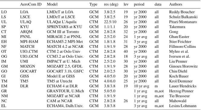
Table 2. Global models with aerosol component modules participating in model assessments.
AeroCom ID Model Type res (deg) lev period data Authors
LO LOA LMDzT at LOA GCM 3.8/2.5 19 yr 2000 all Reddy/Boucher
LS LSCE LMDzT at LSCE GCM 3.8/2.5 19 yr 2000 all Schulz/Balkanski
UL ULAQ ULAQat L’Aquila CTM 22.5/10 26 yr 2000 all Pitari/Montanaro
SP KYU SPRINTARS at KYU GCM 1.1/1.1 20 yr 2000 all Takemura
CT ARQM GCM III at Toronto GCM 2.8/2.8 32 yr 2000 all Gong
MI PNNL MIRAGE 2 at PNNL GCM 2.5/2.0 24 1 yr avg all Ghan/Easter
EH MPI-HAM ECHAM5.2 MPI-Met GCM 1.8/1.8 31 3 yr avg all Stier/Feichter
NF MATCH MATCH 4.2 at NCAR CTM 1.9/1.9 28 yr 2000 all Fillmore/Collins
OT UIO CTM CTM 2 at Oslo Univ CTM 2.8/2.8 40 yr 2000 all Myhre et al.
OG UIO GCM CCM3.2 at Oslo Univ. GCM 2.8/2.8 18 3 yr avg all Iversen et al.
IM UMI IMPACT at U. Mich CTM 2.5/2.0 30 yr 2000 all Liu/Penner
GM MOZGN MOZART 2.5, GFDL CTM 1.9/1.9 28 yr 2000 all Ginoux/Horowitz
GO GOCART GOCART 3.1b, GSFC CTM 2.0/2.5 30 yr 2000 all Chin/Diehl
GI GISS Model E at GISS GCM 4.0/5.0 20 yr 2000 all Koch/Bauer
TM TM5 TM5 at Utrecht CTM 4.0/6.0 25 yr 2000 all Krol/Dentener
EM DLR ECHAM 4 at DLR GCM 3.8/3.8 19 10 yr avg m Lauer/Hendricks
GR GRANTOUR, U.Mich CTM 5.0/5.0 1 yr avg m,aot Herzog/Penner
NM MOZART at NCAR CTM 1.9/1.9 1 yr avg m,aot Tie/Brasseur
NC CAM at NCAR CTM 2.8/2.8 26 1 yr avg all Mahowald
EL ECHAM4, Dalh.Univ. GCM 3.8/3.8 3 yr avg m,aot Lesins/Lohmann
note: only models with AeroCom IDs have submitted data according to the AeroCom request, definition: GCM - Global Circulation model (nudging preferred), CTM - Chemical Transport Model
A future intention of the AEROCOM initiative is that the least constrained “Experiment A” can be revisited to quantify improvements by future efforts in aerosol modeling. More insights on differences in aerosol modeling are expected from “Experiment B”, where model input is harmonized in terms of aerosol emissions for the year 2000. “Experiment Pre” is the counterpart to “Experiment B”, as it provides the reference in estimates of anthropogenic contributions and as-sociated forcing. A comparison and a general assessment of forcing simulations on the basis of these experiments is sum-marized in Schulz et al. (2006). The prescribed AeroCom (component) emissions for “Experiment B” and “Experiment Pre” can be downloaded at ftp://ftp.ei.jrc.it/pub/Aerocom/ . The choices made to arrive at a harmonized emission data set for all major aerosol components are explained in more detail in Dentener et al. (2006). “Experiment Indi” is dif-ferent in that it investigates the sensitivity of modeling and
the model diversity of processes and parameterizations es-sential to estimates of the aerosol indirect effect. Details can be found under http://nansen.ipsl.jussieu.fr/AEROCOM/ INDIRECT/indirect protocol.html.
3 Results
The database consists now of results from twenty modeling groups. Table 2 lists the 16 “Experiment A” AeroCom partic-ipants, who submitted full datasets and 4 contributors, who submitted at an earlier stage (e.g. in Kinne et al., 2003) or provided only partial information.
Here, only results of “Experiment A” are explored, prefer-ably those for the year 2000. Submissions to the three other experiments at this stage are incomplete or in preparation. Simulated properties for aerosol optical thickness (aot) and
1818 S. Kinne et al.: An AeroCom initial assessment
8
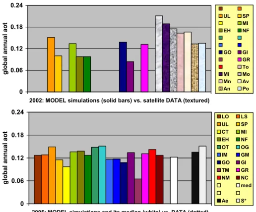
Figure 1. Comparison for the annual global average aerosol optical thickness at .55µm (aot) between simulations in global modeling and data derived from remote sensing measurements. The upper panel shows diversity in 2002 among models and satellite data (Kinne et al 2003). The lower panel displays model diversity in 2005 and compares the model median to two data references from remote sensing: AERONET (Ae) and a satellite-data composite (S*). Spatial deficiencies of remote sensing data-sets in both panels have been corrected with the bias, such sub-sampling would introduce to the model median value.
The lower panel of Figure 1 indicates the two recommended remote sensing based references for the global annual aot at 0.135 (Ae - AERONET) and at 0.151 (S* - satellite composite). The composite value (S*) is based on monthly 3ox 3o longitude/latitude monthly averages,
where preference is given to year 2000 data. Over land preference is given to MISR over TOMS, except in the central tropics, where MODIS is preferred over MISR. Over oceans MODIS is preferred over AVHRR-1ch, whereas this order in reversed at mid-(to high)
0 0.06 0.12 0.18 0.24
2002: MODEL simulations (solid bars) vs. satellite DATA (textured)
gl ob al an nual aot UL SP MI EH NF GO GI GR To Mi Mo Mn Av An Po 0 0.06 0.12 0.18 0.24
2005: MODEL simulations and its median (white) vs. DATA (dotted)
global annual aot
LO LS UL SP CT MI EH NF OT OG IM GM GO GI TM GR NM NC med Ae S*
Fig. 1. Comparison for the annual global average aerosol optical thickness at 55 µm (aot) between simulations in global modeling and data
derived from remote sensing measurements. The upper panel shows diversity in 2002 among models and satellite data (Kinne et al., 2003). The lower panel displays model diversity in 2005 and compares the model median to two quality data references from remote sensing: AERONET (Ae) and a satellite-data composite (S*). Spatial deficiencies of remote sensing data-sets in both panels have been corrected with the bias, such sub-sampling would introduce to the model median value.
aerosol absorption (aab) are compared among models and to measurements from ground-based networks and satellites. Also model differences for aerosol component mass extinc-tion efficiencies (mee) are explored, because this mass to aot conversion factor summarizes model assumptions for aerosol size and water uptake. Simulated global annual averages are addressed first to provide a general overview. Then more insights are provided from regional differences. Finally, sea-sonality issues are addressed.
3.1 Global annual averages
When validating aerosol module simulations on a global scale, it has become customary to compare simulated an-nual global aot values to those obtained from remote sens-ing. Comparisons among model simulations for the (annual and globally averaged) mid-visible aot (at 550 nm) are pre-sented in Fig. 1. Figure 1 demonstrates, how model simu-lations have changed from the work of Kinne et al. (2003) to now. Figure 1 also includes data from remote sensing. Since all remote sensing data are spatially incomplete adjust-ments needed to be applied to make global averages compa-rable. These adjustments involved the spatially and
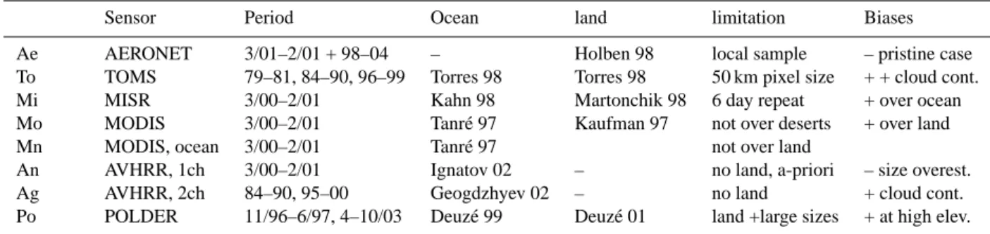
tempo-rally complete median field from modeling. A correction fac-tor for each remote sensing data set was applied from the ra-tio of the model median average over the model median sub-set average, sub-sampled at data locations only. The upper panel presents adjusted global annual averages from TOMS, MISR, MODIS, AVHRR and POLDER retrievals (corre-sponding global aot fields are presented later in Sect. 3). Ta-ble 3 summarizes contributing time-periods, retrieval refer-ences and known biases. Some of these biases were also dis-cussed in recent papers (Myhre et al., 2005; Jeong and Zi, 2005). In the lower panel the number of remote sensing ref-erences is reduced to two, though higher quality, selections: A satellite composite, which combines the regional strength of individual retrievals and an estimate based on statistics at AERONET ground sites.
The lower panel of Fig. 1 indicates the two recommended remote sensing based references for the global annual aot at 0.135 (Ae – AERONET) and at 0.151 (S* – satellite com-posite). The composite value (S*) is based on monthly 3◦×3◦ longitude/latitude monthly averages, where prefer-ence is given to year 2000 data. Over land preferprefer-ence is given to MISR over TOMS, except in the central tropics, where MODIS is preferred over MISR. Over oceans MODIS is
Table 3. Aot data-sets from remote sensing data used in comparisons to models.
Sensor Period Ocean land limitation Biases
Ae AERONET 3/01–2/01 + 98–04 – Holben 98 local sample – pristine case
To TOMS 79–81, 84–90, 96–99 Torres 98 Torres 98 50 km pixel size + + cloud cont.
Mi MISR 3/00–2/01 Kahn 98 Martonchik 98 6 day repeat + over ocean
Mo MODIS 3/00–2/01 Tanr´e 97 Kaufman 97 not over deserts + over land
Mn MODIS, ocean 3/00–2/01 Tanr´e 97 not over land
An AVHRR, 1ch 3/00–2/01 Ignatov 02 – no land, a-priori – size overest.
Ag AVHRR, 2ch 84–90, 95–00 Geogdzhyev 02 – no land + cloud cont.
Po POLDER 11/96–6/97, 4–10/03 Deuz´e 99 Deuz´e 01 land +large sizes + at high elev.
10
Figure 2. An illustration of modeling steps in aerosol components modules of global models –
from emissions(-fluxes) by dust (DU), sulfate (SU), particulate organic matter (POM), sea-salt (SS) and black carbon (BC), via predictions for dry mass (m) and aerosol optical thickness (aot) to estimates of climatic impacts (radiative forcing).
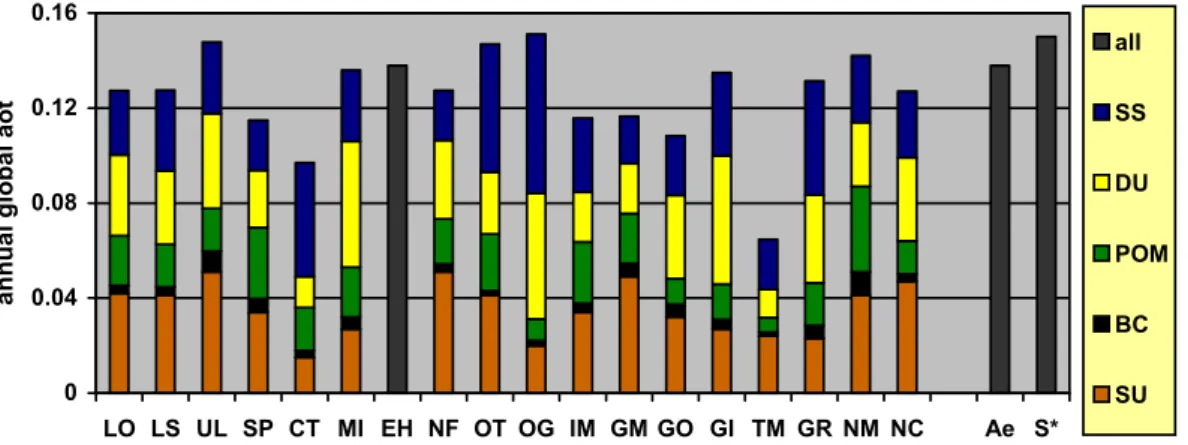
The simulated (aerosol) radiative forcing depends on both: aot and absorption as illustrated in Figure 2. Thus, the commonly tested aot agreement (to data) alone cannot guarantee accurate estimates in radiative forcing. It is possible that the agreement to now available higher quality aot data from remote sensing (see Figure 1) improved so quickly, because each model has enough freedom for any aerosol component to adjust data on (1) emission, (2) processes affecting aerosol lifetime and (3) aerosol size – also via aerosol water uptake? This suspicion is certainly supported by a comparison of aot contributions from the individual sub-components. Figure 3 reveals large model differences in compositional mixture (which has not changed since the last assessment in Kinne et al. 2003). It also demonstrates that the agreement for the sum of all components, which was presented in Figure 1 is a poor measure for overall model skill and model diversity. Model diversity for each of the five component aot contributions individually is significantly larger than for the combined total aot. This is also quantified in Table 4, where annual global averages - on a component basis - are compared among all aerosol modules. In the right-most column of Table 4, the diversity for just the 16 aerosol
Fig. 2. An illustration of modeling steps in aerosol components modules of global models – from emissions(-fluxes) by dust (DU), sulfate
(SU), particulate organic matter (POM), sea-salt (SS) and black carbon (BC), via predictions for dry mass (m) and aerosol optical thickness (aot) to estimates of climatic impacts (radiative forcing).
preferred over AVHRR-1ch, whereas this order in reversed at mid-(to high) latitudes. The AERONET value (Ae) is based on monthly statistics at all (ca. 120) ground-sites, which pro-vided quality data for the year 2000. The density of the land-sites is highest for the US and Europe, but very weak for Northern Africa and Asia (http://aeronet.gsfc.nasa.gov).
Figure 1 shows that the agreement among models im-proved for the global annual aot during the last couple of years. In 2005 the simulated aot (the total aot of all com-ponent combined) on a global annual basis in most models remains within 15% of a value of 0.125. This represents a marked improvement over the initial comparison of eight models in 2002. Most simulated global averages now agree well to both consolidated high-quality data from remote sens-ing (Ae and S* in the lower panel of Fig. 1). This raises the question, if consistency in aerosol processing improved in a similar fashion or if the better agreement largely reflects ad-justments to satisfy tighter constraints by remote sensing.
All participating global aerosol modules in this compar-ison distinguish between five different aerosol components: sulfate (SU), black carbon (BC), particulate organic matter
(POM), dust (DU) and sea-salt (SS). All models simulate (generally from emission inventories) global fields of aerosol component mass. Then this mass is converted into (spec-trally dependent optical) properties of aot and absorption, from which eventually estimates for the aerosol impact on the energy balance are derived (commonly quantified by the radiative forcing). Figure 2 illustrates these successive pro-cessing steps in aerosol modeling.
The simulated (aerosol) radiative forcing depends on both: aot and absorption as illustrated in Fig. 2. Thus, the com-monly tested aot agreement (to data) alone cannot guaran-tee accurate estimates in radiative forcing. Is it possible that the agreement to now available higher quality aot data from remote sensing (see Fig. 1) improved so quickly, be-cause each model has enough freedom for any aerosol com-ponent to adjust data on (1) emission, (2) processes affecting aerosol lifetime and (3) aerosol size – also via aerosol water uptake? This suspicion is certainly supported by a compari-son of aot contributions from the individual sub-components. Figure 3 reveals large model differences in compositional mixture (which has not changed since the last assessment
1820 S. Kinne et al.: An AeroCom initial assessment
11 modules of the AeroCom exercise is summarized by total diversity (TD) and in brackets by central diversity (CD): both TD and CD are defined by the ratio between the largest and smallest average. Thus, a value of one corresponds to perfect agreement and any amount larger than one is the adopted measure of diversity. TD refers to all models, whereas CD refers only to the central 2/3 of all models - as extremes in modeling for CD are excluded.
Figure 3. Individual contributions of the five aerosol components (SS-seasalt, DU-dust, POM-particulate organic matter, BC-black carbon, SU-sulfate) to the annual global aerosol optical thickness (at 550nm). For comparison, two ‘quality’ aot data references from remote sensing are provided: ground data from AERONET and a satellite-composite based on MODIS (ocean) and MISR (land) data. (No apportioning is possible for ‘EH’, due to inter-component mixing).
For aot, the CD of individual components contributions is between 2.0 and 2.7. This is three to six times larger than for the component combined total of 1.3 (which was illustrated by model comparison for 2005 in Figure 1). The largest component CDs for aot are associated with black carbon, dust and sea-salt. CDs for aot-to-mass conversions (mass-extinction-efficiency) indicate (see Table 4) that for sea-salt and dust differences in aerosol size are a major reason for their aot diversity. Aerosol size is not only influenced by assumptions to primary emissions but also by the permitted water uptake, which is controlled by assumptions to component humidification and local ambient humidity. Table 4 indicates that on a global annual basis the simulated aerosol water mass shows strong diversity and aerosol water mass is (at least) comparable to the aerosol dry mass of all sub-components combined. Thus, for the hydrophilic
0 0.04 0.08 0.12 0.16 LO LS UL SP CT MI EH NF OT OG IM GM GO GI TM GR NM NC Ae S* an nua l gl ob al a o t all SS DU POM BC SU
Fig. 3. Simulated contributions of the five aerosol components (SS-seasalt, DU-dust, POM-particulate organic matter, BC-black carbon,
SU-sulfate) to the annual global aerosol optical thickness (at 550 nm) by individual models in global modeling. For comparison, the two quality data references by AERONET (Ae) and by a satellite composite (S*) of the lower panel in Fig. 1 are repeated. (Note: No accurate apportioning is possible for the “EH”-model, due to inter-component mixing). For comparison, two “quality” aot data references from remote sensing are provided: ground data from AERONET and a satellite-composite based on MODIS (ocean) and MISR (land) data. (No apportioning is possible for “EH”, due to inter-component mixing).
Table 4. Comparison of annual global averages for aerosol optical depth (AOT), aerosol dry mass (M) and its ratio (ME) for 20 aerosol
component modules in global modeling.
LO1 LS1 UL1 SP1 CT1 MI1 EH1 NF1 OT1 OG1 IM1 GM1 GO1 GI1 TM1 EM1 GR1 NM1 NC1 EL1 Med2 MaxMin3 M,mg/m2 –SU4 4.2 5.3 1.8 2.1 3.3 3.9 4.6 3.3 3.7 2.8 4.3 5.2 3.8 2.8 1.8 5.1 2.7 4.3 4.7 3.0 3.9 2.9(1.6) –BC4 .35 .43 1.0 .73 .48 .37 .22 .37 .38 .36 .40 .50 .53 .44 .09 .29 .58 .45 .45 .35 .39 11(1.4) –POM4 3.5 3.2 4.1 4.5 5.0 4.0 1.9 3.3 4.0 2.0 3.3 3.1 3.4 2.9 0.9 2.6 2.3 2.8 1.4 3.7 3.3 5.6(1.5) –DU4 26.9 40.1 57.2 34.0 8.8 43.4 16.2 34.0 43.0 46.6 38.1 41.3 57.8 56.6 26.1 18.4 36.2 30.4 34.6 17.7 39.1 6.6(1.8) -SS4 8.9 24.7 12.8 14.4 18.5 10.8 20.4 8.1 18.0 8.9 7.0 6.8 25.8 12.3 4.8 15.8 15.0 25.9 27.5 3.0 12.6 5.4(2.3) –total 44 74 77 56 36 62 43 49 69 60 53 57 92 75 34 42 57 64 64 28 56 2.7(1.7) –water 48 115 55 35 147 255 54 47 36 54 7.1(3.1) –f5 MASS .18 .12 .09 .13 .24 .13 .16 .14 .12 .09 .15 .15 .08 .08 .08 .19 .10 .12 .10 .25 .13 2.9(1.7) r6 POM/BC 10 7.4 4.1 6.2 10.4 10.8 8.6 8.9 10.5 5.5 8.3 6.2 6.4 6.5 10 9.0 4.0 6.2 3.1 10.6 8.4 3.2(1.6) AOT550 nm –SU4 .042 .041 .051 .034 .015 .027 7 .051 .041 .020 .034 .049 .032 .027 .024 .023 .041 .047 .032 .034 3.4(2.0) –BC4 .0033 .0036 .0088 .0058 .0030 .0050 7 .0034 .0020 .0021 .0037 .0056 .0053 .0039 .0017 .0054 .0100 .0031 .0027 .004 5.2(2.7) –POM4 .021 .018 .018 .030 .018 .021 7 .019 .024 .009 .026 .021 .011 .015 .006 .018 .036 .014 .013 .019 5.0(2.1) –DU4 .034 .031 .040 .024 .013 .053 7 .033 .026 .053 .021 .021 .035 .054 .012 .037 .027 .035 .009 .032 4.5(2.5) –SS4 .027 .034 .030 .021 .048 .030 7 .021 .054 .067 .031 .020 .025 .035 .021 .048 .028 .028 .003 .030 3.3(2.3) –total .127 .128 .149 .115 .097 .136 .138 .127 .148 .151 .116 .117 .108 .134 .065 .131 .142 .127 .060 .127 2.3(1.3) –abs .0037 .0062 .0020 .0059 .0044 .0064 .0028 .0061 .0067 .005 3.2(2.2) f5T .45 .48 .52 .42 .37 .30 7 .51 .44 .27 .45 .57 .45 .33 .49 .35 .61 .50 .80 .50 3.1(1.6) Angstrom 0.70 0.68 0.71 0.63 0.97 0.86 0.13 0.48 1.01 .70 7.4(1.8) ME,m2/g SU4 10.2 7.8 28.3 18.0 4.2 6.3 7 17.8 11.1 7.2 7.8 8.5 8.4 9.5 13.3 8.9 9.2 14.5 13.0 8.5 6.7(2.5) BC4 9.4 8.2 8.8 8.0 6.5 13.1 7 9.2 5.3 5.7 9.3 10.4 10.0 8.9 18.9 9.3 15.9 9.1 7.6 8.9 3.5(1.6) POM4 6.4 5.7 4.4 9.1 3.7 5.0 7 4.6 6.0 4.4 8.0 6.3 3.2 5.1 6.7 8.2 11.4 3.9 5.3 5.7 2.8(1.5) DU4 1.38 .88 .70 1.04 2.05 1.62 7 1.07 .60 1.14 .68 .66 .60 .95 0.46 1.24 .98 .99 .52 .95 15.(2.3) SS4 3.10 1.46 2.34 1.51 3.13 3.38 7 1.78 3.05 7.53 4.33 2.37 .97 2.84 4.3 3.44 .90 .88 1.69 3.0 7.7(2.9)
1model abbreviations: LO=LOA (Lille, Fra), LS=LSCE (Paris, Fra), UL=ULAQ (L’Aquila, Ita), SP=SPRINTARS (Kyushu, Jap), CT=ARQM (Toronto, Can), MI=MIRAGE
(Rich-land, USA), EH=ECHAM5 (MPI-Hamburg, Ger), NF=CCM-Match (NCAR-Boulder, USA), OT=Oslo-CTM (Oslo, Nor), OG=OLSO-GCM (Oslo, Nor) [prescribed background for DU and SS], IM=IMPACT (Michigan, USA), GM=GFDL-Mozart (Princeton, NJ, USA), GO=GOCART (NASA-GSFC, Washington DC, USA), GI=GISS (NASA-GISS, New York, USA), TM=TM5 (Utrecht, Net), EM=ECHAM4 (DLR, Oberpfaffenhofen, Ger) [Exp B-data], GR=GRANTOUR (Michigan, USA), NM=CCM-Mozart (NCAR-Boulder, USA), NC=CCM-CAM (NCAR-Boulder, USA), EL=ECHAM4 (Dalhousie, Can) [bold letters indicate models participation in the AeroCom exercise]
2most likely value in modeling: global annual average of the median-ranked model [only the 15 AeroCom models with AOT calculations are considered]
3model diversity measures: ratio of global annual maximum and minimum among (AeroCom) models (in brackets: the ratio without the two largest and smallest model averages) 4aerosol component abbreviations: SU=sulfate, BC=black carbon, POM= particulate organic matter (1.4* OC), OC=organic carbon, DU=mineral dust, SS=sea-salt.
5fine-mode fraction of the total for aerosol dry mass (M) and aerosol optical depth (AOT), where the fine-mode here is approximated by contributions of only SU, BC and POM 6dry mass ratio between particulate organic matter (POM [( 1.4*OC]) and black carbon (BC)
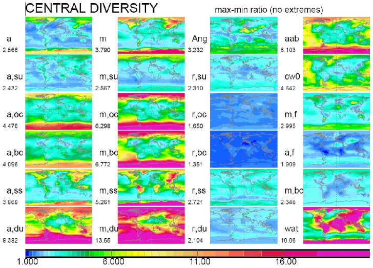
Fig. 4. Global fields for central diversity CD (max/min ratios of the central 2/3 in modeling) for yearly averages (of 16 AeroCom models).
Blue colors indicate better agreement among models, while colors towards yellow or red represent significant local diversity. The left two columns present central diversity fields of aot (a) and dry mass (m) for component combined totals (top panel) and for component contributions of sulfate (su), particulate org. matter (oc), black carbon (bc), sea-salt (ss) and dust (du). Also displayed are diversity fields of component mass extinction efficiency (r), the dry-mass to aot conversion factors. The remaining diversity fields relate to aerosol size (Ang: Angstrom parameter; m,f: dry-mass ratio between fine mode aerosol [su+oc+bc] and total, a,f: aot ratio between fine mode aerosol [su+oc+bc] and total), to aerosol absorption (aab: absorption aot, cw0: co-single scattering albedo [1−w0]), to carbon composition (m, bo: BC/POM dry-mass ratio) and to aerosol water (wat). Values associated with each field provide the area-weighted global annual CD. Note, that model-diversity has the judged in the context of aerosol loading (large diversities in remote regions are less important), thus, corresponding model median fields are provided in the Appendix.
in Kinne et al., 2003). It also demonstrates that the agree-ment for the sum of all components, which was presented in Fig. 1 is a poor measure for overall model skill and model diversity. Model diversity for each of the five component aot contributions individually is significantly larger than for the combined total aot. This is also quantified in Table 4, where annual global averages – on a component basis – are com-pared among all aerosol modules. In the right-most column of Table 4, the diversity for just the 16 aerosol modules of the AeroCom exercise is summarized by total diversity (TD) and in brackets by central diversity (CD): both TD and CD are defined by the ratio between the largest and smallest av-erage. Thus, a value of 1.0 corresponds to perfect agreement and any amount larger than 1.0 is the adopted measure of
di-versity. TD refers to all models, whereas CD refers only to the central 2/3 of all models – as extremes in modeling for CD are excluded.
For aot, the CD of individual components contributions is between 2.0 and 2.7. This is three to six times larger than for the component combined total of 1.3 (which was illustrated by model comparison for 2005 in Fig. 1). The largest component CDs for aot are associated with black carbon, dust and sea-salt. CDs for aot-to-mass conversions (mass-extinction-efficiency) indicate that for (see Table 4) sea-salt and dust differences in aerosol size are a major rea-son for their aot diversity. Aerosol size is not only influenced by assumptions to primary emissions but also by the per-mitted water uptake, which is controlled by assumptions to
1822 S. Kinne et al.: An AeroCom initial assessment component humidification and local ambient humidity.
Ta-ble 4 indicates that on a global annual basis the simulated aerosol water mass shows strong diversity and aerosol water mass is (at least) comparable to the aerosol dry mass of all sub-components combined. Thus, for the hydrophilic com-ponents of sea-salt and sulfate larger model diversities for aot than for dry mass are expected. For global sea-salt CDs, however, this trend is reversed. A possible explanation is the transport of larger sea salt particles in some models, which creates larger diversity near sources, more so for mass than for aot. A contributing factor is also the large sea-salt mass diversity over continents (see discussions in the next section and the presentation of diversity fields in Fig. 4). This illus-trates that even regions with significant lower concentrations can distort the global average and that the reliance on global averages can be misleading. Thus, local diversity fields are explored next.
3.2 Annual fields
Given the short-lived nature of aerosol, evaluations at suf-ficient resolution in time and space will allow more useful insights into issues of aerosol global modeling. To extend the model diversity assessments of Table 4, local CDs for 24 annual fields are presented in Fig. 4. All models were interpolated to the same horizontal resolution of 1◦×1◦ lat-itude/longitude. At each grid point all models were ranked according to the simulated magnitude into a probability dis-tribution function (PDF). The ratio between the 83% and the 17% values of the PDF (such that extremes in modeling are ignored) define the CDs in Fig. 4. It can be seen that model diversity usually increases towards remote regions, largely due to differences in transport and/or aerosol processing (e.g. removal). However, diversity has to be judged also in the context of the absolute concentration, as larger diversities are less meaningful in regions of overall low concentrations. Global fields of the model median (the 50% value of the PDF) are presented in figures of the Appendix, where Fig. A1 corresponds to Fig. 4.
Model diversity is usually larger over land than over oceans for total dry mass and total aot. The largest differ-ences occur in central Asia and extend eastwards to western regions of North America. Sub-component diversity is usu-ally stronger, but component diversity patterns differ. For sulfate the diversity for aot is increased over mass diversity at low latitude land regions and in the continental outflow re-gions. Large model diversity for aerosol water may provide an explanation. For organic and black carbon the diversities are usually larger than for sulfate. Particular large are car-bon diversities over some oceanic regions. This location over the ocean for the rather insoluble organic particles suggests model differences in transport and removal processes which affect the transport to remote regions. As differences in trans-port strongly contribute to model diversity, it does not sur-prise that for dust, whose global distributions are largely
de-fined by transport, display larger diversities away from dust source regions. The fact that dust diversity (and sea-salt di-versity over oceans) for aot is significantly smaller than for mass could indicate deliberate choices for size with the goal to match expectations. However, it should be pointed out, that different cut-off assumptions for the largest dust and sea-salt sizes create mechanically larger diversity for mass than for aot because the largest particles contribute a lot to mass but little to aot. The size-diversity for dust and sea-salt is also demonstrated in larger diversities for mass-to-aot conversion factors (the r-panels in the third column of Fig. 4), compared to carbon or sulfate species. Also, the largest model diversity for aerosol size, illustrated via the Angstrom parameter (label “Ang”), occurs in regions, where dust (Northern Africa and Asia) and sea-salt (southern mid-latitudes) are the dominant components.
A comparison of the panels in the upper corners of Fig. 4 between aerosol optical depth (label “a”) and its fraction as-sociated with absorption (label “aab”) illustrates that sity for aerosol absorption is significantly larger than diver-sity for aerosol optical thickness. This indicates that reduced uncertainties in aerosol direct forcing require primarily im-provements to the characterization of the local (or regional) aerosol composition. Larger diversities for absorption occur towards remote regions. This suggests that aerosol process-ing durprocess-ing long-range transport is a key issue for reductions of model diversity. Emissions which dominate the diversity near the sources over land seem to be more homogeneous in models, probably because similar emission inventories are used by different modeling groups.
3.3 Comparisons to observational data
Although model diversity is of interest, it is not necessarily a measure of the real uncertainty. Similar assumptions or ap-proaches in modeling can overshadow real uncertainties, as for example in the case of moderate diversity found for par-ticulate organic matter (organic carbon mass) despite large uncertainties for its emission factors, secondary production, humidification and absorption.
Model diversity is of limited value without quality ref-erence observations, which from now on is referred to as data, for simplicity. Unfortunately, reference data are only available for a few (and often integrated) properties. And even if data exist, they usually suffer from limitations to (of-ten poorly defined) accuracy and from restrictions of spatial and/or temporal nature. Subsequent comparisons focus on two properties that are critical in the context of aerosol radia-tive forcing: mid-visible values for aerosol optical thickness (aot) and its fraction linked absorption, the aerosol absorp-tion optical thickness (aab). Two data references based on year 2000 measurements were adopted.
The first data (local) reference is provided by quality as-sured data of sun-/sky-photometer robots distributed all over the world as part of the AERONET network (Holben et al.,
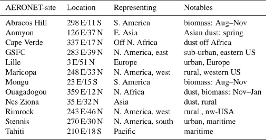
Table 5. AERONET references for monthly statistics of mid-visible aot and absorption aot.
AERONET-site Location Representing Notables
Abracos Hill 298 E/11 S S. America biomass: Aug–Nov
Anmyon 126 E/37 N E. Asia Asian dust: spring
Cape Verde 337 E/17 N Off N. Africa dust off Africa
GSFC 283 E/39 N N. America, east sub-urban, eastern US
Lille 3 E/51 N Europe urban, Europe
Maricopa 248 E/33 N N. America, west rural, western US
Mongu 23 E/15 S S. America biomass: Aug–Nov
Ouagadogou 359 E/12 N N. Africa dust, biomass: Nov–Jan
Nes Ziona 35 E/32 N Asia dust, rural
Rimrock 243 E/46 N N. America, west rural , nw-USA
Stennis 270 E/30 N N. America, south urban, maritime
Tahiti 210 E/18 S Pacific maritime
1998). Direct solar attenuation samples provide highly accu-rate data for aot. In addition, aab estimates are derived from less frequent sky-radiance sampling. However, to achieve a sufficient signal to noise ratio, aab data are only reliable at larger aot values (Dubovik et al., 2002). The association to a specific location can introduce biases when used as regional reference, because global modeling has a coarse horizontal resolution on the order of 200×200 km (see Table 2). In particularly, sites dominated by local pollution or sites near mountains are expected to introduce unwanted biases with respect to the regional average. Thus, comparisons were lim-ited to 12 sites, where local biases are believed to be small. Site details in Table 5 indicate that the selected 12 sites cover a variety of aerosol types and regions.
The second (regional) data reference is established by a satellite aot retrieval composite (S*). It combines individ-ual retrieval strength, giving regional preferences separately over land and ocean surfaces. Over land MISR is preferred over TOMS, except in the central tropics, where MODIS is preferred over MISR. Over tropical oceans MODIS is pre-ferred over AVHRR (1channel), while at mid-(to high) lati-tudes AVHRR (1 channel) is preferred over POLDER. The basis for the preferred regional retrieval choice and its next best substitute is provided in Table 6. In Table 6 regional annual retrieval averages are compared to AERONET based averages for the same region. Regional choices are based on climatological zones in each hemisphere and surface type (ocean, coast or land). To allow comparisons (on a regional basis), spatial sub-sampling of any data set was overcome by using the complete coverage of the median model. For each data-set, its regional average was adjusted, by multiplying it with the ratio of averages from modeling for the same re-gion. This ratio was defined of by the average involving all regional pixels over the average involving only those pixels that contributed to the regional data average. These adjusted regional annual averages are listed in Table 6 and allow a
di-rect comparison. Among all satellite retrievals, that with the minimum difference to the (adjusted) regional AERONET average was selected to contribute to the satellite composite S*.
3.3.1 Global
For a first impression on model performance in general, rel-ative aot deviations of the model median to the satellite com-posite (S* in Fig. 5) are presented on a monthly basis in Fig. 6. Values of +1/−1 indicate over-/under-estimates of 100%, with respect to the satellite reference.
Most noticeable are model overestimates for Europe dur-ing the summer months. This trend even extends durdur-ing the late summer into Northern Asia. Other median model bi-ases are the too early biomass burning season in South Amer-ica, too much dust in Northern Africa during the winter sea-son, and aot underestimates in tropical regions. Given that satellite retrievals over oceans are less uncertain than over land, the large discrepancy to modeling over tropical oceans is puzzling. More quantitative comparisons for regions of Fig. 7 are given in Table 6. Table 6 lists the regional aver-ages of the satellite composite (S*) and compares them to spatial adjusted AERONET averages (Ae), to those of indi-vidual satellite retrievals (see Table 3) and to the median in global modeling (med).
3.3.2 Regional and local
Comparisons in this section are illustrated in a similar format. For selected locations and regions, monthly averages are presented in a clock-hourly sense (12–1: January, . . . , 11–12: December). Purple (sectional) disks indicate monthly data at a magnitude according to the disk-size in the lower right. Following the same magnitude scale, green lines illustrate the mean in modeling, while blue and yellow sections indicate ranges between maximum and minimum
1824 S. Kinne et al.: An AeroCom initial assessment
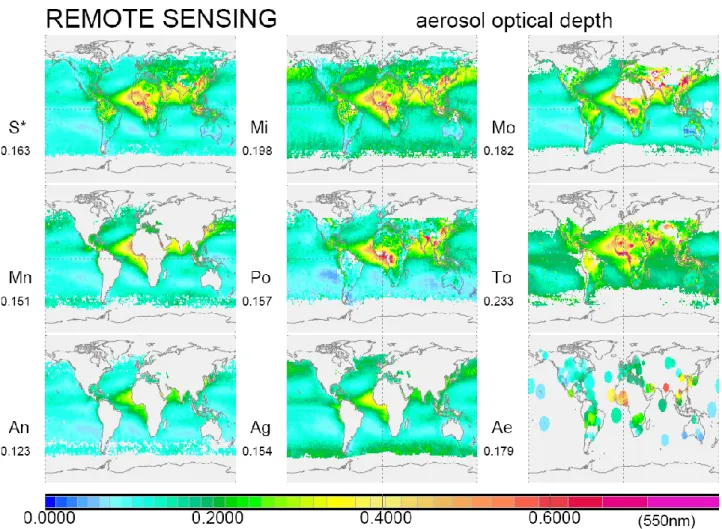
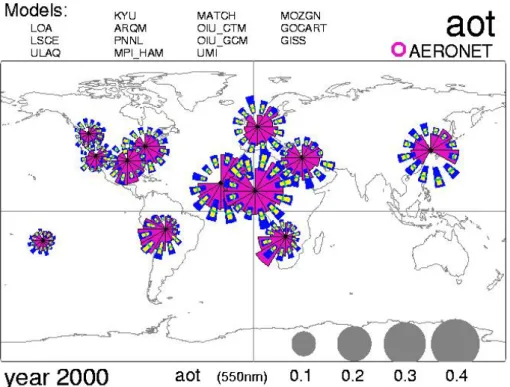
Fig. 5. Comparison of annual global fields for the mid-visible (550 nm) aerosol optical depth from remote sensing. These include available
multi-annual retrievals from different satellite sensors of MODIS (Mn, Mo), MISR (Mi), TOMS (To), Po (Polder) and AVHRR (Av, Ag) – for more details see Table 3. Based on high quality samples of AERONET (Ae, which have been artificially expanded for better visualization in the lower right panel) regional retrieval choices lead to a satellite composite (S*, upper left panel). Over oceans Mn is preferred in the tropics and An is preferred at high latitudes. Over land Mi is preferred except for the tropical biomass belt, where Mo is the first choice. Values below labels indicate global area-weighted annual averages of all available data. Due to spatial sampling differences, a direct comparison of these values is not possible without an adjustment, which was done with help of the median model in Table 6. Table 6 also provides the rationale for regional retrieval preferences in S*.
in modeling in reference to all models (TD) and central-2/3 models (CD). Disagreement is apparent, when the yellow range of modeling is completely within or outside the purple area of the data.
Aot data
Simulated aot values are compared locally in Fig. 8 at 12 sites to AERONET statistics and regionally in Fig. 9 for 21 (highlighted) regions to the satellite retrieval composite.
The two main model biases common to both data-references are (1) too large aots over Europe and (2) a too early biomass burning season in South America. Other mod-eling biases with respect to the two reference data do not match: AERONET suggests that models (1) underestimate
the strength of the tropical biomass burning season, (2) over-estimate Eastern Asia contributions in off-dust seasons and (3) overestimate during US winters. The satellite compos-ite suggests that (1) simulations are too low over tropical oceans, (2) the seasonality peak for central Asia is reversed and (3) dust transport from Asia to North America is too low. In light of retrieval issues, there is less confidence in biases to satellite over land. However, aot underestimates of most models to MODIS over tropical oceans are significant. Un-fortunately, ground data are too sparse to clarify this issue.
The intra-regional standard deviation for aot is compared in Fig. 10. Dust and dust-outflow regions display the largest aot variability in modeling. Common to most models is a stronger variability over (1) central Asia during summer and fall (related to dust), (2) Eastern Asia, (3) Northern
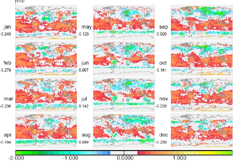
Fig. 6. Local relative deviations for aot of the (16 AeroCom) models median with respect to the satellite composite (S*) of Fig. 5 on a
monthly basis: (S* – model)/S*. Blue to green indicate an overestimate and red to yellow an underestimate of the medina model. In light of satellite retrieval errors deviations with 25% (corresponding to a 0.25 value) are ignored.
Africa and (4) Europe, during winters. Variability is weaker over (1) North America and (2) Southern Africa during the biomass season. Most models display significantly stronger inter-regional variability for monthly aot averages than the satellite reference. An explanation in part, is the spatial limitation of satellite retrievals, as essential periods of the seasonal cycle are excluded (e.g. no retrievals over snow cover in winter at mid-latitudes), although discrepancies are largest in regions, where retrievals are difficult and often sparse to start with.
Absorption data
Aerosol absorption is best quantified by the product of aot and co-single scattering albedo, the absorption aot (aab). Local comparisons at AERONET sites are given in Fig. 11.
Models overestimate absorption strength in the Eastern US and in the Mid-East. On the other hand tropical biomass absorption strength is underestimated and the peak occurs
too early in South America. Notable are disagreements for the central African AERONET site, where the simulated (biomass) absorption at year’s end is too large, but too weak in the opposite season.
Values for aab were only provided by about half of the models. To capture the diversity for the absorption potential involving all models a different approach was selected by de-riving for all models the mid-visible (.55 µm) imaginary part of the Refractive Index (RFi) from simulated component dry mass contributions. For the total RFi, assumed component RFi values (0.0015 for dust, 0.03 for particulate organic mat-ter, 0.6 for black carbon and zero for all other components) were multiplied by corresponding fractional volume weights and combined with aerosol water (of the model median) con-tributions to RFi. Regional and monthly RFi statistics of Ae-roCom models are presented in Fig. 12.
The modeled absorption potential is strongest in the tropi-cal biomass regions, with a seasonal peak which occurs prior to the seasonal peak for aot. Also the absorption potential
1826 S. Kinne et al.: An AeroCom initial assessment
Table 6. Regional aot averages of the model median (med) and of remote sensing data from ground (Ae) and space (To,Mi,Mo,Ag,An,Po).
Individual space-sensors have different regional aot retrieval capabilities, as best agreements to ground remote sensing (Ae) are highlighted. Based on regional strengths of individual aot retrievals a satellite composite (S*) was formed.
zonal reg surface % med Ae S* To Mi Mo Ag An Po
global All % 100.0 .122 .135∗ .151* .220∗ .189 .182∗ .172∗ .138∗ .143∗ 1 50–90 N ocean 47 5.53 .106 .076∗ .089* .234∗ .130∗ .126∗ .139∗ .077* .097∗ 2 30–50 N ocean 45 5.98 .148 .122∗ .131 .224∗ .238 .177∗ .165 .130 .154∗ 3 8–30 N ocean 61 10.95 .128 .109∗ .177 .208∗ .220 .178* .159 .146 .173∗ 4 8 N–25 S ocean 70 19.75 .079 .131∗ .133 .197 .179 .134* .139 .119 .146∗ 5 25–55 S ocean 87 17.28 .095 .060∗ .111 .204∗ .167 .132∗ .140 .101 .103∗ 6 55–90 S ocean 70 6.31 .088 no data .076* .158∗ .138∗ .106∗ .148∗ .070∗ .064∗ 7 30–50 N coast 19 2.51 .222 .173∗ .195 .277∗ .231 .287∗ .212∗ .153∗ .144∗ 8 8–30 N coast 15 2.75 .204 .199∗ .280 .351 .297 .324 .231∗ .217∗ .218∗ 9 8 N–25 S coast 13 3.50 .106 .200∗ .207 .337 .258 .228 .206∗ .160∗ .199∗ 10 25–55 S coast 6 1.18 .080 .103∗ .106 .221 .124 .136∗ .123∗ .082∗ .081∗ 11 50–90 N Land 53 6.16 .112 .102∗ .114* .223∗ .109* .149∗ .154∗ .074∗ .083∗
12 30–50 N Land 36 4.81 .200 .155∗ .206 .240∗ .206 .321∗ no data no data .151∗
13 8–30 N land 24 4.34 .348 .377∗ .333 .358 .330 .448∗ no data no data .240∗
14 8 N–25 S land 17 4.83 .136 .194∗ .252 .282 .243 .248 no data no data .172∗
15 25–55 S land 7 1.36 .086 .075∗ .098 .181∗ .098 .148∗ no data no data .112∗
16 55–90 S land 30 2.73 .018 no data no data .143∗ .201∗ .051∗ no data no data .024∗
note: a * indicates a spatial sampling correction with the aot field of the median model
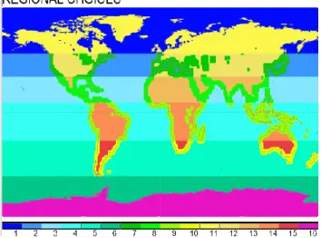
Fig. 7. Regional choices for aot-comparison among modeling and
remote sensing. A distinction was made between land- ocean- and coastal surfaces for selected zonal bands.
is larger for Europe than for Asia or North America. Rela-tive low is the absorption potential for the Eastern U.S. Low-est values are modeled for ocean regions away from sources. However, the main point is that there is significant model di-versity for the absorption potential as a consequence from large difference in aerosol composition. This diversity is at least as large as the diversity for aot (see also Fig. 4).
3.3.3 Discussion
Larger values for aot over Europe are probably related to emission overestimates in older inventories, which were gen-erally used in modeling. Similarly, the too early biomass burning season in South America strongly suggests the use of incorrect emission data. The biases found here provide an additional motivation for the AeroCom “Experiment B”, where updated emissions are required to be used as model input. More difficult are explanations for aot discrepancy in remote regions of tropical and Southern Hemisphere oceans between modeling and satellite retrievals, which are believed to have good cloud-detection capabilities, such as MODIS. Although absolute aot differences generally do not exceed 0.1, relative differences often exceed a factor of two. It re-mains unclear, if deviations are to be blamed on modeling (e.g. transport) or retrieval error (e.g. cloud contamination). Unfortunately, surface observations currently are too sparse to clarify this issue in the southern ocean regions.
In terms of aerosol absorption, it should be pointed out, that there are large differences in aerosol composition among models. The absorption potential of sub-components dif-fers strongly. Thus, significant absorption differences among models are expected. However, only a few models provided data on single scattering albedo (ω0), as a measure of
spe-cific absorption, from (less clear) assumptions to component absorption or water uptake. Thus, to demonstrate diversity of all models, fixed values for component absorption and water uptake (of the model median) were assumed and RFi
21
Figure 8: Comparisons of monthly average mid-visible aot data between local statistics at
AERONET sites (of Table 4) and model simulations. Monthly data are presented in a clock-hourly sense (12-1: Jan, 1-2: Feb, , 11-12: Dec). Purple pie disk sections indicate AERONET data according to the grey disks in the lower right. For (locally interpolated) simulations (of models listed on top) at the same scale, green lines indicate averages, maximum-minimum ranges among all models are in blue and those of just the central 2/3 models are in yellow.
The two main model biases common to both data-references are (1) too large aots over Europe and (2) a too early biomass burning season in South America. Other modeling biases with respect to the two reference data do not match: AERONET suggests that models (1) underestimate the strength of the tropical biomass burning season, (2) overestimate Eastern Asia contributions in off-dust seasons and (3) overestimate during US winters. The satellite composite suggests that (1) simulations are too low over tropical oceans, (2) the seasonality peak for central Asia is reversed and (3) dust transport from Asia to North America is too low. In light of retrieval issues, there is less confidence in biases to satellite over land. However, aot
Fig. 8. Comparisons of monthly average mid-visible aot data between local statistics at AERONET sites (of Table 4) and model simulations.
Monthly data are presented in a clock-hourly sense (12–1: January, 1–2: February, , 11–12: December). Purple pie disk sections indicate AERONET data according to the grey disks in the lower right. For (locally interpolated) simulations (of models listed on top) at the same scale, green lines indicate averages, maximum-minimum ranges among all models are in blue and those of just the central 2/3 models are in yellow.
underestimates of most models to MODIS over tropical oceans are significant. Unfortunately, ground data are too spare to clarify this issue.
Figure 9: Comparisons of mid-visible aot data between the satellite retrieval composite (see S*
in Figure 5) and simulations for 21 high-lighted regions. (Symbols are explained in Figure 8.)
The intra-regional standard deviation for aot is compared in Figure 10. Dust and dust-outflow regions display the largest aot variability in modeling. Common to most models is a stronger variability over (1) central Asia during summer and fall (related to dust), (2) Eastern Asia, (3) Northern Africa and (4) Europe, during winters. Variability is weaker over (1) North America and (2) Southern Africa during the biomass season. Most models display significantly stronger inter-regional variability for monthly aot averages than the satellite reference, although discrepancies are largest in regions, where retrievals are difficult and often sparse to start with.
Fig. 9. Comparisons of mid-visible aot data between the satellite retrieval composite (see S* in Fig. 5) and simulations for 21 high-lighted
regions. (Symbols are explained in Fig. 8.)
1828 S. Kinne et al.: An AeroCom initial assessment
23
Figure 10: Comparisons of mid-visible aot intra-regional standard deviation between the
satellite retrieval composite (S* in Figure 5) and simulations within 21 high-lighted regions. (Symbols are explained in Figure 7).
3.3.2.2. absorption data
Aerosol absorption is best quantified by the product of aot and co-single scattering albedo, the absorption aot (aab). Local comparisons at AERONET sites are given in Figure 11.
Fig. 10. Comparisons of mid-visible aot intra-regional standard deviation between the satellite retrieval composite (S* in Fig. 5) and
simu-lations within 21 high-lighted regions. (Symbols are explained in Fig. 7).
Figure 11: Comparisons of monthly mean mid-visible absorption (aerosol) optical depth
[aot*(1-ω0)] between local statistics at AERONET sites (of Table 5) and model simulations. (Symbols are explained in Figure 8).
Models overestimate absorption strength in the Eastern US and in the Mid-East. On the other hand tropical biomass absorption strength is underestimated and the peak occurs too early in South America. Notable are disagreements for the central African AERONET site, where the simulated (biomass) absorption at year’s end is too large, but too weak in the opposite season. Values for aab were only provided by about half of the models. To capture the diversity for the absorption potential involving all models a different approach was selected by deriving for all models the mid-visible (.55µm) imaginary part of the Refractive Index (RFi) from simulated component dry mass contributions. For the total RFi, assumed component RFi values (0.0015 for dust, 0.03 for particulate organic matter, 0.6 for black carbon and zero for all other components) were multiplied by corresponding fractional volume weights and combined with aerosol water (of the model median) contributions to RFi. Regional and monthly RFi statistics of AeroCom models are presented in Figure 12.
Fig. 11. Comparisons of monthly mean mid-visible absorption (aerosol) optical depth [aot*(1-ω0)] between local statistics at AERONET
sites (of Table 5) and model simulations. (Symbols are explained in Fig. 8).
25
Figure 12: Model inter-comparisons of mid-visible refractive index imaginary parts (models
listed on top) on a regional basis. Estimates are based on dry mass volume weights, model median aerosol water and prescribed dry component imaginary parts: They are .0015, .03 and .6, for dust, particulate organic matter and black carbon, respectively and zero for sea-salt and sulfate. Monthly data are shown in a clock-hourly sense (12-1: Jan, 1-2: Feb, …, 11-12: Dec). The model median is purple, the average is green and simulation-ranges are blue (all models) or yellow (central models).
The modeled absorption potential is strongest in the tropical biomass regions, with a seasonal peak which occurs prior to the seasonal peak for aot. Also the absorption potential is larger for Europe than for Asia or North America. Relative low is the absorption potential for the Eastern US. Lowest values are modeled for ocean regions away from sources. However, the main point is that there is significant model diversity for the absorption potential as a consequence from large difference in aerosol composition. This diversity is at least as large as the diversity for aot (see also Figure 4).
Fig. 12. Model inter-comparisons of mid-visible refractive index imaginary parts (models listed on top) on a regional basis. Estimates are
based on dry mass volume weights, model median aerosol water and prescribed dry component imaginary parts: They are .0015, .03 and .6, for dust, particulate organic matter and black carbon, respectively and zero for sea-salt and sulfate. Monthly data are shown in a clock-hourly sense (12–1: January, 1–2: February, . . . , 11–12: December). The model median is purple, the average is green and simulation-ranges are blue (all models) or yellow (central models).
for individual models were derived based on volume weights (using data on component mass). Regional comparisons for RFi were presented in Fig. 12 and demonstrate the (poten-tially – due to fixed values) large model diversity for absorp-tion. (Further Ri conversion into ω0(Ri is proportional to
[1–ω0]) failed, because this conversion is size dependent (e.g.
coarser aerosol is associated with larger values for [1–ω0] for
the same RFi). For models that provided values for ω0,
sim-ulated absorption strength can be compared to local statis-tics of AERONET, from the ratio of aab (Fig. 11) and aot (Fig. 8). Based on these ratios, models underestimate the spe-cific aerosol absorption over industrial areas in North Amer-ica and Europe. (only very large aot overestimates lead to total absorption overestimates in Europe). A location of the AERONET sites near sources of pollution and the expected bias to more absorption at low aot values in AERONET ra-diance data inversion (e.g. see the Tahiti site in Fig. 11) are potential explanations, but underestimates for BC emissions in the models cannot be ruled out either.
4 Conclusion
Comparisons of aerosol properties simulated by newly de-veloped aerosol component modules for/in global modeling have demonstrated a surprising good agreement for the
an-nual global aerosol optical depth, quite in agreement with re-cent efforts to obtain improved remote sensing observations. However, the notion that uncertainties for the (aerosol) direct forcing have reduced in a similar way are premature. This aot agreement is not supported on a sub-component level for aerosol optical depth and even less for component aerosol dry mass and aerosol water from which these (component) aerosol optical depths are derived. The large differences in compositional mixture for aerosol dry mass and water uptake affect aerosol absorption. Thus, despite general agreement for aot, strong diversity for aerosol absorption will introduce large uncertainties to the aerosol associated solar radiative (direct) forcing. In particular, uncertainties for the climate forcing term (the changes for the solar energy balance at the top of the atmosphere) will be large, because this term repre-sents a difference of two values with similar magnitude but opposite in sign (a loss term due to solar scattering and a gain term due to aerosol absorption). To summarize: Good ment for total aot (-fields) does not guarantee good agree-ment for aerosol forcing and diversity for total aot among models is an insufficient measure for forcing diversity.
In the initial AeroCom “Experiment A” comparisons, models were allowed the input of their choice. Diversity patterns are large enough, to recommend further investiga-tions into modeling differences. Better constraints to input in
1830 S. Kinne et al.: An AeroCom initial assessment
Fig. A1. Annual median fields of global modeling for aerosol properties, corresponding to diversites (and notation) of Fig. 4. For better
viewing each field is scaled, whereby the value below each label indicates to the multiplier to the linear scale at the bottom. Aerosol dry mass in the 2nd column and aerosol water in the lower right panel are is in units of g/m2and the mass extinction efficiencies in the 3rd column are in m2/g. All other properties are without units.
“Experiment B” and “Experiment Pre” should enhance cur-rent capabilities to reveal strength and weaknesses on issues associated with aerosol processing and aerosol transport. The AeroCom effort has developed a transparent strategy to doc-ument overall model diversity and individual model bias to a multitude of observational data. Further progress for model evaluations is expected in the near future from more capa-ble data sensors (e.g. active remote sensing from space for vertical profiles [A-train]), higher temporal and spatial reso-lution (e.g. more capable geostationary satellites [MSG]) and new and improved ground (e.g. AERONET) and in-situ (e.g. commercial airlines) networks. On the other hand, as aerosol modules in global modeling strive to include more processes and feedbacks, the complexity of aerosol modules will in-crease, and so will the need for more specific measurement detail.
Appendix A
Global reference fields for aerosol properties from modeling
Given the short lifetime of quite different types and processes of aerosol, there is a need for reliable references on regional and seasonal distributions of aerosol properties in the global context. Observational data-sets (e.g. from remote sensing) should be the first choice. But measurements are only avail-able for a few often integrated properties. And even then these data are usually spatial and temporal restricted and/or suffer from severe accuracy limitations.
Aerosol modules in global modeling can provide complete and consistent global fields for all aerosol properties. Rather than relying on one single module, here the whole suite of all 16 modules participating in the AeroCom is the basis to the reference data on aerosol properties. The data presented
Fig. A2. Monthly median fields in global modeling for the mid-visible aerosol optical depth.
1832 S. Kinne et al.: An AeroCom initial assessment
Fig. A4. Monthly median fields in global modeling for the Angstrom parameter based on simulated aerosol optical depths a mid-visible
(0.55 µm) and a near-IR (0.865 µm) wavelength.
Fig. A5. Monthly median fields in global modeling for aerosol mass in g/m2. (Mass is dominated by larger particles, thus mainly reflecting distributions of dust and sea-salt.)