HAL Id: halshs-02563356
https://halshs.archives-ouvertes.fr/halshs-02563356v2
Preprint submitted on 19 Jan 2021
HAL is a multi-disciplinary open access
archive for the deposit and dissemination of
sci-entific research documents, whether they are
pub-lished or not. The documents may come from
L’archive ouverte pluridisciplinaire HAL, est
destinée au dépôt et à la diffusion de documents
scientifiques de niveau recherche, publiés ou non,
émanant des établissements d’enseignement et de
Optimal Prevention and Elimination of Infectious
Diseases
Hippolyte d’Albis, Emmanuelle Augeraud-Véron
To cite this version:
Hippolyte d’Albis, Emmanuelle Augeraud-Véron. Optimal Prevention and Elimination of Infectious
Diseases. 2021. �halshs-02563356v2�
WORKING PAPER N° 2020 – 21
Optimal Prevention and Elimination of Infectious Diseases
Hippolyte d’Albis
Emmanuelle Augeraud-Véron
JEL Codes: I18, C61, E13
Optimal Prevention and Elimination of
Infectious Diseases
1
Hippolyte d’ALBIS
2Paris School of Economics, CNRS
Emmanuelle AUGERAUD-VÉRON
3GREThA, University of Bordeaux
January 18, 2021
1We are grateful to Andrés Carvajal and the Special Editors of this issue, two
anonymous referees, and to Jean-Pierre Amigues, Eric Benoît, Martial Dupaigne, Al-bert Marcet and participants in seminars at Universities of Exeter, Paris and Toulouse, at European University Institute and ETH Zurich for their valuable comments and suggestions. The usual disclamer applies.
2
Correspondence: 48 boulevard Jourdan, 75014 Paris, France. E-mail: hdal-bis@psemail.eu
3Correspondence: 6 avenue Léon Duguit, 33600 Pessac, France. E-mail:
Abstract
This article studies the optimal intertemporal allocation of resources devoted to the prevention of deterministic infectious diseases that admit an endemic steady-state. Under general assumptions, the optimal control problem is shown to be formally similar to an optimal growth model with endogenous discounting. The optimal dynamics then depends on the interplay between the epidemiological characteristics of the disease, the labour productivity and the degree of inter-generational equity. Phase diagrams analysis reveal that multiple trajectories, which converge to endemic steady-states with or without prevention or to the elimination of the disease, are feasible. Elimination implies initially a larger prevention than in other trajectories, but after a …nite date, prevention is equal to zero. This “sooner-the-better” strategy is shown to be optimal if the pure discount rate is su¢ ciently low.
JEL Classi…cation: I18, C61, E13
1
Introduction
Infectious diseases constitute major health issues for which there is large con-sensus on the legitimacy of governments interventions. Yet few analysis has been undertaken to determine the socially optimal allocation of resources to control the evolution of the disease. In this article, we derive a welfare criterion from individual preferences and give precise foundations on a generally held belief, according to which intervention should begin as soon as possible and involve large expenses. We focus our analysis on expenditure that reduce the number of contacts relevant for infection transmission per unit of time and, con-sequently, reduce the spread of the disease. They include prevention campaigns that modify individuals’ behaviors, by e.g. the di¤usion of masks or condoms that reduce the probability of a contact to be infectious, and any measures that reduce physical contacts such as lockdowns of populations. Throughout the ar-ticle, all those policies will be named as prevention measures, and the aim will be to determine the optimal intensity over time of the prevention in a economy that faces an infectious disease.
Infectious disease’prevention is a legitimate topic for economics since, as ar-gued by Bloom and Canning [10], there is little doubt that resource constraints play an important role in the spread of the disease. Moreover, as other diseases, they importantly a¤ect labor and capital markets, and thus growth. However, and despite the fact that past diseases were recognized as economic tragedies,
Gersovitz and Hammer [28] pointed out that it is only since the 1990’s that economists have entered the …eld. The interest has skyrocketed recently with the Covid-19 outbreak. Most articles in the literature adopt a positive approach focusing on private behaviors, such as individual choices on self-exposure to the risk (as in Geo¤ard and Philipson [30] and Kremer [39]), health expenditure (Momota et al. [42]), human capital accumulation (Bell and Gersbach [6], Cor-rigan et al. [20] and Boucekkine et al. [13]), fertility (Young [51]), income distribution ([14]) or biodiversity (Bosi and Desmarchelier [11]). Some papers analyzes the e¤ect of public policies on private behavior (e.g. Geo¤ard and Philipson [31]), while others consider optimal policy correcting for the obvious externalities produced by infectious diseases (e.g. Gersovitz and Hammer [29], Francis [25], Gersovitz [27], Bethune et al. [9] or Eichenbaum et al. [23]).
While few papers in economics adopt a normative perspective, one observes there exists an abundant mathematical epidemiology literature, which dates back from Bernouilli [8]! Following Sethi [47] and Wickwire [50], it is common to use optimal control techniques to de…ne the desirable timing of vaccination, screening or health promotion campaigns. In most cases these studies use as a criterion a convex combination of the dynamic costs of the control and of the number of infected individuals. Moreover, the time horizon is usually …nite and, in analytical models, the problem is linear with respect to the control. Based on this approach Behncke [7] …nds that the optimal control of an epidemics is, in general, such that the prevention e¤ort is maximal on some initial time
interval and then set to zero (see also Buonomo et al. [17] Morris et al. [43]). When the case of disease elimination is considered, the problem is more complex since terminal conditions are free (Barrett and Hoel [5]). Some economic studies (in particular Gersovitz and Hammer [28], Francis [25], Feichtinger et al. [24], Alvares and al. [2] or Rowthorn and Toxvaerd [46]) have used a slightly more sophisticated criterion as they consider the present discounted value of total income net of the costs of the disease and of the control.
We propose an optimal control model in the tradition of Ramsey [45], Cass [18] and Koopmans [38] in which the whole population is a¤ected by an infectious disease, whose dynamics is rather general while admitting an endemic steady-state. The social welfare function is the present discounted value of the product of individual utility and the size of the population. We notably show how this criteria relies on preferences. The introduction of population in the objective is key to avoid the problem stressed by the optimal population literature (see notably Dasgupta [21]) about maximizing the welfare of alive individuals only. By considering an endogenous population in the welfare function, our work distinguishes itself and extends important theoretical contributions of Del…no and Simmons [22], Boucekkine et al. [12], Goenka and Liu [32] or Goenka et al. [34], who in most cases consider speci…c epidemiological processes and study local dynamics. It also complement works such as those of Gersovitz and Hammer [29] or Eichenbaum et al. [23], who proceed by simulations.
which is of pure exchange, i.e. without physical capital, which allow us to com-pletely characterize the model despite a general formulation for the dynamics of the infectious disease. The dynamics of the optimal prevention then depends on the interplay between the epidemiological characteristics of the disease, labour productivity and intergenerational equity. We believe it’s important to charac-terize the global dynamics of the optimal system as it permits to visualize both the objective that should be reached in the short run, and some trajectories that could be hidden while performing local long-run analysis.
We …nd that it may be optimal to reduce the prevalence rate of the infectious disease in the long run only if labour productivity is above some minimal level. If this threshold is not reached, prevention is then at best temporary, simply slowing down the spread of the infectious disease. However, it may not be optimal to undertake temporary prevention. When instead labour productivity is su¢ ciently high, permanent allocation of resources to prevention is feasible though not necessarily optimal. If permanent prevention is socially optimal, the prevention e¤ort monotonically increases with time for low initial prevalence rate, and is hump-shaped or decreasing otherwise. Hence, our paper establishes that under a welfare criterion for social intertemporal optimization a “sooner-the-better” strategy may not be the optimal one, in contrast to Behncke [7]. This statement is however reversed when we consider paths that may yield to the elimination of the infectious disease. We …rst show that a simple modi…cation of usual deterministic models describing endemic infectious diseases can be made
to allow for elimination in …nite time.1 Trajectories that drive to elimination are
characterized by an increasing prevention for a …nite interval of time and, once the infectious disease is eliminated, the prevention is zero. We show that upon existence, such paths are optimal if the pure discount rate is su¢ ciently small. In that case, it consequently is socially desirable that prevention should begin as soon as possible. Moreover, the e¤ort initially devoted to prevention is larger for elimination than for any other dynamics. This is a theoretical foundation for a “whatever it costs” response to a disease outbreak.
We begin by presenting the dynamics of the population a¤ected by an infec-tious disease in section 2. The epidemiological assumptions are put forward and discussed using standard examples of HIV and ‡u. In section 3 we set up the so-cial planner’s problem, then prove the existence of a solution and characterize it. The dynamics of the optimal prevention is analyzed in section 4. The question on whether it is socially optimal to eliminated the infectious disease is studied section 5, and illustrated with a hand solved example. Section 6 concludes.
2
Dynamics of the infectious disease
This section presents the general characterization of the dynamics of the disease that encompasses a number of models proposed in the epidemiological litera-ture. It’s a two-compartment model in which the total population is allowed
1Note that stochastic models are usually considered to explain why …nite time elimination
of the disease is possible (Britton [16], Allen and Lahodny [1]). Contrary to what happens with deterministic models, it is there possible that the disease never breaks out when a small number of infectives are initially present in the whole population, even if the reproduction number is greater that one.
to change with the prevalence rate. The evolution of the disease is constrained by some assumptions that are satis…ed, for instance, in classical compartmental models (Kermack and Mac Kendrick [37]). We also propose to introduce an arbitrarily small threshold below which the disease is considered as eliminated. This modelling feature will be key in the subsequent analysis.
2.1
A two-class framework
Time is continuous and indexed by t 2 R+. The population at time t, whose size
is denoted Pt, is a¤ected by an infectious disease and is thus decomposed in two
classes of individuals: the susceptible, who are healthy, and the infected, who may transmit the disease. The number of individual of each class is respectively
denoted St > 0 and It 0, and satisfy: Pt = St+ It. It will be convenient
to de…ne the relative share of infected individuals with respect to share of
sus-ceptible ones as follows: at = It=St. This ratio is a monotonically increasing
transformation of the traditional prevalence, given by: It=Pt= at= (1 + at), and
will be named as the prevalence index throughout the remaining of the paper.
Moreover, we consider the following general law of motion for at:
_at= g (ht; at) at; (1)
where the dot indicates the …rst derivative with respect to time and where ht
stands for the per capita expenditure devoted to the disease’s control. These expenditure can be interpreted as prevention campaigns and any preventive measures that reduce the number of contacts relevant for infection transmission
per unit of time and, consequently, reduce the spread of the disease (see, for instance, Castilho [19]). Note that these expenditure can not stand for vacci-nation campaigns or screening and isolation strategies, as they produce a third class of individuals within the population; a case that is not considered here. In the rest of the paper, htwill be referred as the level of prevention at time t.
The growth rate of the prevalence index, characterized by function g, is supposed to satisfy:
H1. g : R2
+! R, is C2, g10(ht; at) < 0, g20 (ht; at) < 0 and g1100 (ht; at) > 0: There
exist a > 0 and h > 0 such that g (0; a ) = g (h ; 0) = 0.
Assumption H1 fully describes the kind of disease we are dealing with. The
growth rate of the prevalence index is supposed to decrease with at which, of
course, does not imply a monotonic relationship between _at and at. If there is
no prevention, the disease lasts forever but stabilizes within the population: the prevalence index converges to the endemic state a . The other steady-state, given for a = 0, and named in the epidemiological literature the disease-free equilibrium, can easily be check as being unstable as Assumption H1 implies
g (0; 0) > 0. The reproduction number2, i.e. the number of secondary cases
that can appears when one infected individual is added in a population of fully susceptible individuals for the duration of her illness, denoted R0, is here larger
2Formally, we can write: ag (h; a) = F (h; a) + V (a) where F include the terms related
to the transmission of the disease and V those related to other causes (death, etc.). The derivative at a = 0 of the pervious equation is given by: g (h; 0) = F0(h; 0) + V0(0). Then
the (controled) reproduction number is de…ned as Rc= F0(h; 0)=V0(0), while the (classical)
than 1 (van den Driessche [49]). Figure 1a represents this dynamics. 6 -g(0; at)at at a -
-Figure 1a: The dynamics ofatwhenht= 0
Prevention may modify the dynamics of the disease. To …x ideas, let
as-sume that ht is an exogenous constant. If this constant belongs to (0; h ), the
prevalence index converges to another stable steady-state characterized by a prevalence rate that is lower than a ; the reproduction number with positive
control Rcremains larger than 1. However, if the constant is larger than h , the
disease dynamics are dramatically modi…ed as the prevalence index converges to zero; the control is su¢ cient to eliminate the disease in the long run and
we now have Rc < 1. Figure 1b illustrates such dynamics with two di¤erent
exogenous ht: h12 (0; h ) and h2> h . In the remaining of the paper, ht will
be the control variable optimally chosen by a benevolent social planner.
6 -g(h1; at)at at a -6 -g(h2; at)at at a
Figure 1b: The dynamics ofatwhenht> 0
dynamics. An alternative dynamics without prevention could be obtained by
assuming: a < 0. Such an disease would not exhibit an endemic
steady-state. The unique stable steady-state being the one with a zero prevalence index. Prevention may then be used to accelerate the convergence process. Moreover, assuming that a ! +1, allow to consider a disease whose prevalence inde…nitely increases if there is no control of it.
By de…nition, the population growth rate writes as follows: _ Pt Pt = 1 1 + at _ St St +I_t It at ! : (2)
For computational reasons, we assume that the growth rate is characterized by a function denoted n (:) that satis…es:
H2. _Pt=Pt= n (at). n : R+! [n
¯; n (0)], is C
2, n0(a t) 0.
Assuming that the population growth rate does not depend on (St; It; ht) is
rather strong but is widely used in the epidemiological literature, notably in the examples presented below. Moreover, the assumption concerning non positivity of n0(at) is not only more realistic -infectious diseases increase the death
rates-but also, as it will be discussed throughout the paper, more meaningful.
2.2
A minimal threshold for infectious diseases
We now consider a simple generalization of equation (1), which is given by:
_at=
g (ht; at) at if at> amin
0 if at amin;
where 0 amin 1. Equation (3) introduces a threshold below which the
infec-tious disease is considered as eliminated. The threshold can be arbitrarily low and below it the infectious disease can not survive and spread within the pop-ulation. Above this threshold, the dynamics has the same qualitative property as the one we have considered before (Assumption H1 is left unchanged).
Tech-nically, the main di¤erence between the case amin > 0 and the case amin = 0
that is usually considered in the epidemiology literature, is that steady-state
amin can be reached in …nite time, which will appear as a key property below.
We will then assume that when amin is reached, the disease is eliminated.
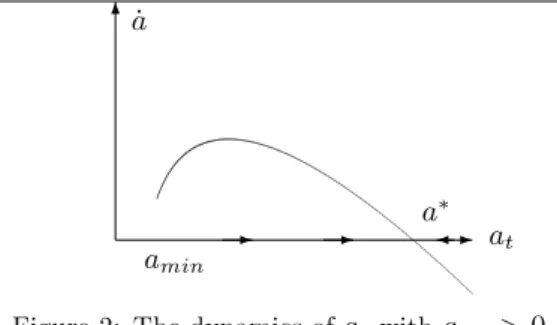
The dynamics of at is represented in Figure 2, in the case of no prevention.
6 -_a at a -amin
Figure 2: The dynamics ofatwithamin> 0
Our framework generalizes most works in economics that have analytically studied the optimal dynamics of an infectious disease: Del…no and Simmons [22], Gersovitz and Hammer [28] and Barrett and Hoel [5] study a dynamics similar to (1), but for a function g which is speci…ed, while Boucekkine et al. [12] consider a shock on the initial stock of the population describing an infectious disease with instantaneous e¤ects and no endemic steady-state.
2.3
Examples
Our assumptions on functions g and n are now confronted to two examples presented e.g. in Zhou and Hethcote [52]: a SI model, which can describe the HIV (similar to May and Anderson [40]) and a SIS model, which can describe a ‡u. In SIS models, infected individuals may recover for the disease but are not immunized and may again be infected. This is relevant for ‡u if one considers a mutating virus. However, most current models of the SARS-CoV-2 assume this is not the case and use three-compartments models of the SIR type (Avery et al. [4]). Such models can be covered by our analysis provided that the size of the population is kept constant.
Example 1. SI model (HIV)
Let us …rst suppose that amin = 0 and ignore the possibility to control the
disease. The natural growth rate of the susceptible population is given by ,
where > 0 and > 0 respectively stand for the birth and the death rates,
while the growth rate of the infected population is ; parameter 0
measures the over-mortality yield by the disease. Both vertical and horizontal
transmission are considered: …rst a proportion 2 [0; 1] of the children of
infected people are born healthy, while the others are infected. Moreover, as in May and Anderson [40], it is assumed that the transmission is given by a frequency-dependent transmission function: transmission is proportional, up to
The dynamics of each subpopulation is therefore given by: _ St = ( ) St+ It St It St+ It ; (4) _ It = [ (1 ) ] It+ St It St+ It : (5)
It can be easily shown that this system does not generically admit a steady-state
except: St = It = 0. Hence, the dynamics of the disease is better understood
using per capita variables or, equivalently, by using our prevalence index at
(de…ned as at= It=St). Using (4) and (5), the dynamics of at solves:
_at= [ at] at; (6)
which is a logistic equation. Therefore, if 2 (0; 1], the dynamics of atwrites:
at=
( )
a0
a0+ ( ) a0 e ( )t
: (7)
Equation (6) admits (i) two steady-states if > + : namely, ^a = 0, which
is unstable and a = ( ) = , which is stable, (ii) one steady-state if
+ : namely, ^a = 0, which is stable. Consequently, if the
transmis-sion coe¢ cient is su¢ ciently low, the infectious disease ultimately disappears.
Conversely, if is high, the disease survives as the prevalence index stabilizes.3
If there is full vertical transmission (i.e. if = 0), the only possible steady state
is ^a = 0, whose stability is given by the sign of .
3Alternatively, one may present the stability results using the reproduction number which
is here given by R0= ( ) = :The dynamics of a can be rewritten as:
_at= R0 1 at at ;
Using (4) and (5), the population growth rate n (at) solves:
n (at) =
at
1 + at
; (8)
which decreases in at; moreover, n (at) < . The higher bound
for n (:) being the population growth rate without infectious disease.
Suppose now that prevention may a¤ect the disease dynamics through the transmission parameter by reducing the number of e¤ective contacts by time
unit. Let ht be the per capita expenditure devoted to prevention and the
transmission coe¢ cient at time t be a function that writes (ht) and satis…es
0(h
t) < 0. The dynamics of at is now given by:
_at= [ (ht) at] at: (9)
It is immediate to check that Assumption H1 is satis…ed only if > 0 and if
(0) > + and that Assumption H2 is always satis…ed. Hence, full vertical
transmission is excluded here.
Remarkably, our example easily extends to the case amin > 0, for which
equation (7) holds for at amin only. The stability analysis is modi…ed as
follows: if > + , a remains a stable steady-state while if < + ;
amin is stable and can be reached in …nite time.
Example 2. SIS model (Flu)
dynam-ics for the susceptible and the infected: _ St = (St+ It) St+ It St It St+ It ; (10) _ It = ( + + ) It+ St It St+ It : (11)
The main di¤erence are that there is no vertical transmission of the disease,
and that infected individuals recover at rate > 0: Then, the dynamics of the
prevalence index satis…es:
_at= [ at( + )] at; (12)
while the population growth rate is the same as (8). The stability analysis is
similar to that of the previous example.4 Again, we can assume that is a
decreasing function of the level of prevention h.
3
The optimal control problem
This section establishes the optimal control problem we are going to study. It is an in…nite horizon framework with an economic structure and the population dynamics described in section 2. We …rst present and discusses the social welfare function and then prove the existence of an optimal solution.
3.1
The social welfare function
The social welfare function we introduce is derived from the aggregation of individual’s preferences. Each individual is supposed to belong to a dynasty
4The reproduction number is now given by R
0= = ( + + )and the dynamics of the
prevalence index can be rewritten as:
_at= ( + + ) R0 1 at
+ + + at:
of altruistic individuals. Without infectious diseases, the growth rate of the dynasty is equal to n (0). However, at each point of time, members of a given dynasty may die from the disease, which reduces the growth rate of the dynasty.
We denote by t the probability as of time t = 0 that the dynasty is still
alive at time t. If alive at time t, the utility of a dynasty member depends on
consumption ctand is independent of the health status. The utility function is
denoted u (ct). If not alive at time t, the utility is supposed to be a constant
that is normalized to the value of the utility with non consumption: u (0) :
Importantly, we suppose that u (0) 1. The expected utility of the dynasty
at time t = 0 is therefore:
Z +1
0
e ( n(0))t[ tu (ct) + (1 t) u (0)] dt; (13)
where is the pure discount rate which satis…es the following restriction:
H3. > n (0) :
Moreover, function u satis…es the following assumption:
H4. u : R+ ! R+, u 2 C3, u0 > 0, u00< 0 and limc!0u0(c) = +1.
To obtain the social welfare function, we assume that the population is composed
by a continuum of identical dynasties, whose total size at time t = 0 is P0.
By the law of large numbers, the probability t is, at the aggregate level, the
ratio between the size of the population and the size that would prevail in the
absence of infection. Thus: t = Pt=P0en(0)t = e
Rt
welfare function at time t = 0 is therefore simply obtained by multiplying the function (13) by the initial size of the population P0, and rearranging to obtain:
P0
Z +1
0
e R0t[ n(as)]ds[u (ct) u (0)] dt + P0u (0)
n (0): (14)
Maximizing this latter function is, in fact, equivalent to maximizing:
Z 1
0
e tPtu (ct) dt: (15)
The social planner function is thus the discounted value of the product of the size of the population, Pt, and of the instantaneous utility of each individual. In
this total utilitarism (i.e. Bentamite) function, we observe that for a given path of consumption, a larger population increases the social welfare. Consequently,
the assumption n0(a
t) < 0, implies that reducing the number of infected
indi-viduals increases welfare, everything being equal. Observe …nally that the limit case n0(a
t) = 0, which features infectious diseases that have no impact on the
population growth, implies t= 1 and a standard objective function. We notice
that most theoretical works (by most notably Boucekkine et al. [12], Goenka and Liu [32], Goenka et al. [34] or Rowthorn and Toxvaerd [46]) consider either that the infectious disease has no impact on population growth or that the popu-lation does not enter the social welfare function. Del…no and Simmons [22] is an exception as they assume that the disease dynamics impact the instantaneous utility but they do not provide a theoretical foundation for their speci…cation.
3.2
The social planner’s program
The social planner faces the resource constraint of the economy. There is one material good produced using labor and it is assumed that the productivity of an infected individual is lower than the one of an susceptible individual. Production per capita is assumed to be a function of prevalence that is written
as f (at) where is a measure of the productivity of labor and f is a measure
of the quantity of labor. It is assumed that labor is a decreasing and concave function of prevalence: f (:) > 0; f0(:) < 0 and f00(:) 0. The produced good can be used for consumption or for the expenditure devoted to the control of the infectious disease. The resource constraint written in per capita units is therefore:
ct+ ht= f (at) : (16)
Moreover, consumption, prevention and the prevalence index should be non negative. The program of the social planner is to maximize (15) subject to (1) and (16). It writes: max ht Z 1 0 e R0t (as)dsu ( f (a t) ht) dt; s:t: _at= g (ht; at) at if at> amin 0 if at amin;
0 ht f (at) and a02 (amin; a ) given.
(17)
where (at) := n (at). We note that since n is a decreasing function and given
Assumption H3, one has (:) > 0 and 0(:) > 0. As discussed in Boucekkine et
growth model with endogenous discounting.
To reduce the length of the proofs and to focus on the meaningful cases, we
solved the problem for a0 2 (amin; a ) but the analysis can be generalized to
a0> a . Let us notice that the problem is trivial if the initial prevalence of the
infectious disease is below the minimal threshold (i.e. a0 amin): the optimal
consumption is equal to the production f (amin) and the prevention is equal
to zero.
The intertemporal trade-o¤ is the following: an increase in ht yields a
re-duction of both the immediate per-capita consumption and the prevalence of the infectious disease. The latter implies …rst an increase in future per-capita production and therefore the expenditure devoted to prevention can be under-stood as an investment. Moreover, reducing prevalence leads to a modi…cation of the spread between the discount rate and the population growth rate. As
0(a
t) > 0, an increase in htimplies a reduction of the spread, meaning a more
equal treatment between individuals of di¤erent generations as it increases the weight associated to the utility of future generations.
3.3
An existence result
The program (17) is a non autonomous problem with endogenous discounting but can be equivalently analyzed as an exogenous discounting problem using the virtual time method described by Uzawa [48]. The following results are then derived.
Lemma 1 There exists an optimal solution to program (17). The optimal so-lution satis…es ht< f (at).
Proof. See Appendix.
We now turn to the characterization of the solution by analyzing …rst the
case such that amin= 0, which is standard in mathematical epidemiology. The
main goal is to characterized the dynamics of the optimal prevention strategy. Then, we turn to the case amin> 0 to analyze the issue of elimination.
4
Is prevention optimal?
This section studies the system of equations (18) that characterizes the dynam-ics of prevalence and prevention when there is no minimal threshold for the
infectious disease (i.e. for amin = 0). Local dynamics around steady-state are
…rst studied and a geometrical analysis using phase diagrams is then provided.
4.1
The optimal dynamics for
a
min= 0
Let us …rst give the equations describing the optimal trajectories.
Lemma 2 An optimal path is necessarily a solution of the following system:
8 > > < > > : _at= g(ht(a;att))at _ht= (ht;at;ct)
(at) u00 ( f (at) ht)u0 ( f (at) ht)+
g0011(ht;at) g01(ht;at)
if ht> 0;
_at= g(0;a(att)a)t if ht= 0;
with ct= f (at) ht and: (ht; at; ct) = f0(at) u00(ct) u0(ct) + g00 12(ht; at) g0 1(ht; at) + 0(a t) (at) g (ht; at) at + f0(at) + u (ct) u0(ct) 0(a t) (at) g01(ht; at) at g20 (ht; at) at+ (at) : (19)
Proof. See the Appendix.
From Lemma 2, it is straightforward to derive the optimal dynamics of con-sumption, which is always positive (see Lemma 1).
4.2
Prevention in the long run
Let us …rst consider the local dynamics in the neighborhood of the steady-states of (18). We de…ne a ‘corner steady-state’as a steady-state for which the optimal prevention is zero and an ‘interior steady-state’as a steady-state for which the optimal prevention is positive.
Given Assumption H1, the pairs (a ; 0) and (0; 0) are the two corner steady-states of our system. The …rst one satis…es the following properties:
Lemma 3 Provided that there exists an optimal path that converges to the
cor-ner steady-state (a ; 0), it satis…es ht= 0 for t large enough.
Proof. See the Appendix.
Whatever its initial dynamics, the optimal prevention is thus equal to zero after a …nite date if the prevalence index converges to an endemic steady-state without
prevention. The intuition is that (a ; 0) is not a steady-state for the interior dynamics of system (18). Optimal prevention may hence not converge to zero but only reach zero in a …nite time. Since it is never optimal to reach a in a
…nite time, we conclude that ht = 0 in the neighborhood of (a ; 0). Note that
this argument rules out local indeterminacy. This results con…rms the initial …ndings of Goenka et al. [34] who provide conditions for local uniqueness in a setting in physical capital.
Concerning the second corner steady-state, we obtained the following:
Lemma 4 There is no optimal path that converges to (0; 0) :
Proof. See the Appendix.
The disease elimination is not a possible output of models with a traditional representation of infectious diseases. The intuition, which is illustrated in the phase diagrams below is the following. A trajectory that would converges to
the disease-free-equilibrium would necessary imply _ht > 0 forever, which is
not possible because of the budget constraint. The same result is obtained by Rowthorn and Toxvaerd [46] in a similar setting. Below, we show how going beyond this basic statement as we obtain a trajectory leading to elimination that can be optimal.
Let us now study interior steady-states, upon which prevention is positive. Using (18), such a steady-state is a pair (a; h) that satis…es a 2 (0; a ) ; h 2
(0; f (a)) and solves: g (h; a) = 0; (20) [g20 (h; a) a (a)] = f0(a) + u (c) u0(c) 0(a) (a) g 0 1(h; a) a; (21)
where c = f (a) h. Then, a necessary condition for existence of an interior
steady-state is the positivity of equation (21)’s right hand side, which rewrites as follows:
d da
u ( f (a) h)
(a) < 0: (22)
Condition (22) means that the discounted welfare of a generation in the long run should be increased by a reduction of the disease. The increase in
util-ity implied by a marginal decreases of a (measured by f0(a) u0(c) = (a))
should be larger than the negative impact on the endogenous discount (given
by 0(a) u (c) = ( (a))2). Necessary and su¢ cient conditions (20) and (21) may
be rewritten in the following way:
u0(u ( f (a) (a))) (a) = d _a dh d da u ( f (a) (a)) (a) ; (23)
where (a) is the implicit relation between h and a derived from Assumption H1.
The contemporaneous desutility induced by a marginal increase in prevention should equal the bene…ts of the reduction of the prevalence of the disease.
The following lemma studies the existence of interior steady-states.
Lemma 5 i) There exists > 0, such that there is no interior steady-states
^. iii) Upon existence, interior steady-states are locally unstable.
Proof. See the Appendix.
Lemma 5 shows the importance of labor productivity, or equivalently, of the level of wealth per capita, on the prevalence index in steady-state: there are thresholds below which there is an high prevalence and no prevention, and above which there is lower prevalence with some prevention. The intuition of this result hinges on the concavity and on the Inada condition imposed on the utility function: when the average production is low, resources are exclusively devoted to consumption since a marginal decrease of it produces a large desu-tility and since the marginal impact of prevention is independent of the level of productivity. Consequently, an interior steady-state is more likely to exist if the labor productivity is increased: the immediate marginal desutility of prevention (i.e. the LHS of (23)) is then lowered while its impact on future generations’ discounted utility (i.e. the RHS of (23)) is increased.
Importantly, interior steady-states are locally unstable. As it will be done be-low, it is possible to characterize, under further conditions, saddle-path steady-states. Hence, from Lemmas 3 and 5, we conclude there are at most two kinds of paths that converge to a steady-state. First, we have a family of paths con-verging to corner states. Second, upon existence of a saddle-path steady-state, we have the stable arm converging to one interior steady-state. All paths are candidates for optimality. We note that in related settings, the multiplicity
of interior steady-states was established and studied in Del…no and Simmons [22], Goenka and Liu [32] and Goenka et al. [34]. In particular, Goenka et al. [34] give conditions for local uniqueness and show that complex dynamics can occurs. In an decentralized economy with endogenous growth, Goenka and Liu [33] show the existence of multiple steady-state that feature either sustained growth or poverty trap. The optimal health policy is larger in the former than in the latter.
Suppose now there exists at least one saddle-path steady-state. Let us com-pare the unique path that converges to this steady-state to the family of those which converge to the corner steady-state.
Lemma 6 Suppose there exists a saddle-path interior steady-state, denoted by
a; h . The stable arm that converges to a; h may not be optimal.
Proof. See the Appendix.
Lemma 6 shows that the existence of an interior steady-state does not implies that the stable arm is necessarily optimal. In the proof, we show that using a particular case where the long run cost of prevention is higher that the bene…t in terms of production of having a lower share of infected individuals. Then, there exist sets of initial condition such that the intertemporal utility yield by the stable arm is lower than the one yield by the path converging to the corner steady-state. Conversely, there exists initial conditions, upon which the saddle-path is always preferred to those converging to the corner steady-state.
4.3
The global dynamics of prevention
We now propose a geometrical representation of the results that have been previously established by drawing the phase diagram associated to the system of equations (18). To reduce the length of the proofs, an additional set of restrictions is assumed:
H5. g00
12(h; a) = 0, and u000(c) =u00(c) u00(c) =u0(c).
Assumption H5 is su¢ cient to ensure that isocline _h = 0; derived from
func-tion given in equation (19) is well de…ned for g > 0. The disease dynamics
considered in Assumption H1 is now constrained by further assumptions on the
impact of prevention on _at: it is now convex and proportional to at. Moreover,
the utility function restricts to a representative individual with absolute risk aversion lower than absolute prudence, a property satis…ed by standard utility functions including those with harmonic absolute risk aversion. We established the following properties.
Lemma 7 i) The _a = 0 locus is downward slopping in the plane (a; h) and
is such that _a > 0 below the locus. ii) For g > 0; the _h = 0 locus is
de-…ned by a function h = (a) that satis…es lima!0 (a) = 1 and is such
that _h > 0 above the locus. iii) As increases, the _h = 0 moves upward in
(a; h) 2 R2; g (h; a) > 0 .
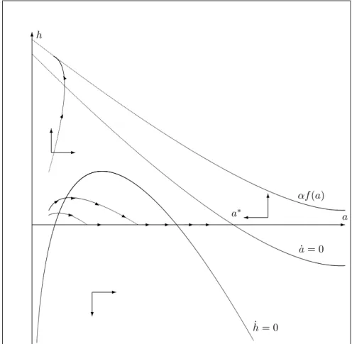
Lemma 7 gives enough information to draw the phase diagram associated to system (18). Depending on the existence of interior steady-states, optimal paths can hence be represented. Possible phase diagrams are given by …gure 3a if there is no interior steady-states and by …gure 3b if there are two interior steady-states.
6 -a h _a = 0 a _h = 0 -? -6 6 - - -j j -* f (a) -K
Figure 3a: Possible trajectories when there is no interior steady-state
Note that we have represented the upper limit for h, given by function f (a),
above the _a = 0 locus, but it as well can be below for some value of a. For
an initial condition a02 (0; a ), there is hence a family of feasible paths: they
converge toward the corner steady-state (0; a ) and provided that the _h = 0 locus is above the horizontal axis, a positive level of prevention is possible for
a …nite interval of time. The di¤usion of the disease may be slowed down for a while but, ultimately, the prevalence index reaches the long-run level with no intervention. Another family of paths is drawn in Figure 3a: they move to the vertical axis with a high level of prevalence. These paths are however not feasible since the prevention monotonously increases with time and reaches in
…nite time the upper limit given by f (a). The consumption is there equal to
zero and, consequently, the path is not optimal.
Labor productivity, which has been shown in the previous section to be crucial for the existence of interior steady-states, has an impact on the dynamics.
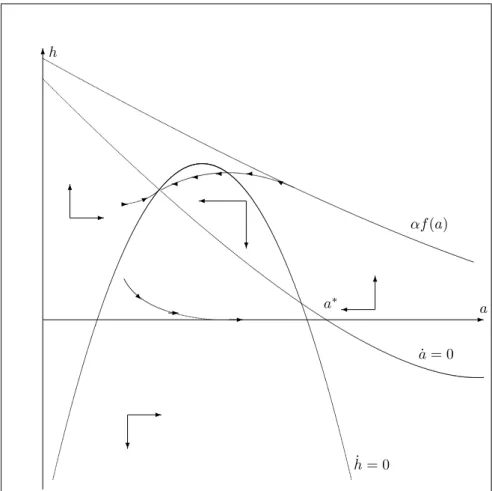
Geometrically, as increases, the _h = 0 locus and the constraint f (a) move
up. Since the _a = 0 locus is left unchanged, interior steady-states are more likely to appear, as stated in lemma 5 and drawn in Figure 3b.
Two interior steady-states are represented in the phase diagram of Figure 3b: a …rst one with a higher level of prevention and a lower prevalence, which is saddle-path and a second one which is a repulsive cycle. Hence, in addition to the families of paths that have been considered in the case without interior states, there is a unique path that converges to the saddle-path steady-state. Remark that if there exist more than two interior steady-states, the phase diagram would exhibit alternatively saddle-paths and cycles. If the stable arm converging to the steady-state h; a is optimal, the prevention monotonically
increase with time if a0 < a and can be an hump shaped function of time if
6 -a h _a = 0 a _h = 0 -? -6 6 ? Y * -R - -f (a)
Figure 3b: Possible trajectories when there are two interior steady-states
In this phase diagram analysis, we have insisted on the fact that on the neighborhood of the vertical axis, the growth rate of prevention is always positive (i.e. _h > 0). This behavior is induced, using (18), by the assumption of a "not too concave" relationship between the infectious disease growth rate and the prevention. More precisely, it is true if:
lim h!0 g00 11(h; 0) g0 1(h; 0) < u00( f (0)) u0( f (0)); (24)
Note …nally that any path that may converge to the vertical axis, and thus to the elimination of the infectious disease, necessarily reaches in …nite time the resource constraint and is therefore not optimal. Assuming the opposite inequality than that of (24) would not change the statement about the impos-sibility to eliminate, but simply the phase diagram. In the next section, we assume that amin> 0, which allows to consider the elimination of the infectious
disease.
5
Elimination of infectious diseases
Lemma 4 has shown that elimination was not possible in the case a amin= 0. We
now consider the case with a positive threshold below which the infectious dis-ease remains constant at a negligible prevalence rate. Below, we …rst show that a trajectory that converges to amin> 0 is feasible and then give the conditions
for its optimality.
5.1
The trajectory toward elimination
We start with the following result.
Lemma 8 An optimal path that converges to the corner steady-state (amin; 0)
may exist. It satis…es ht= 0 for t large enough.
Proof. See the Appendix.
If amin > 0 is allowed, the elimination is feasible in our model. Since amin can
no impact when at= amin.
5.2
Global dynamics with elimination
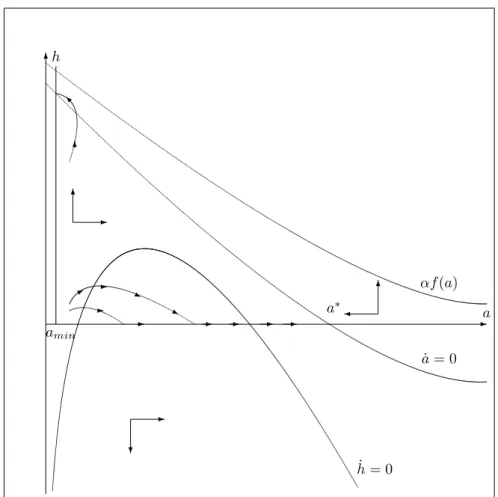
Let us now see how our phase diagrams are modi…ed: a new feasible path appears, which yields to the elimination of the infectious disease in …nite time. Figure 4a represents a possible phase diagram when there is no interior steady-state. 6 -a h _a = 0 a _h = 0 -? -6 6 - - -j j -* f (a) -6 I amin
Figure 4a: Elimination with no interior steady-state
The family of paths that converges to the corner steady-state (0; a ) is still represented in Figure 4a. Moreover, there is a path that reaches the vertical axis in …nite time, along which prevention monotonically increases. Moreover,
the path is unique as it necessarily goes through the intersection between the vertical line at aminand the _a = 0 locus. A necessary condition for the existence
of such a path is simply that those coordinates are feasible, meaning that the
h such that g h; amin = 0 satis…es the following condition: h < f (amin). A
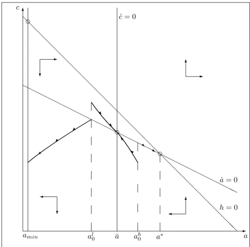
path leading to elimination also appears when there are interior steady-states, as it is shown by Figure 4b. 6 -a h _a = 0 a _h = 0 -? -6 6 ? Y * -R - -f (a) 6 I amin
Figure 4b: Elimination with two interior steady-states
In the following lemma, we give a condition for the optimality of the elimination of the infectious disease.
in-fectious disease. There is a threshold for the pure discount rate, denoted , such
that for < , this path is optimal.
Proof. See the Appendix.
When elimination is achieved, the discounted utility of generation t, which is given by u (ct) = (at), is the highest possible since there is no prevention and
the prevalence index is zero. This however implies that generations that have lived before the elimination have supported large reduction of their welfare due to the necessarily high levels of prevention devoted to the control of the disease. The path that yields to elimination is thus optimal if the pure discount rate is su¢ ciently small. In a rather di¤erent setting, Barrett and Hoel [5] show that elimination is optimal if the exogenous cost of the control is not too large. In our setting, the cost is endogenous and satis…es a budget equation. Our result rather hinges on the comparison of intertemporal utilities. By comparing intertemporal pro…ts of obtained by various vaccination strategies, Geo¤ard and Philipson [31] also show that the discount rate is a key variable but they show that elimination is preferred if discounting is large.
5.3
A hand solved example
Let us illustrate our dynamics with a simple example that encompass the two cases described in Section 2. Concerning the infectious disease, we …rst assume
that the over-mortality rate of infected persons is zero ( = 0), which
of parameters, we assume n (0) = 0, which simply means that the death rate equals the birth rate. While unrealistic, those assumptions are often made in theoretical works (see e.g. Rowthorn and Toxvaerd [46]). We notice that both restrictions are consistent with H1 and H3. We also suppose that the impact of
prevention on the infectious contacts is linear by writing: (h) = 0 h; and
assuming that h 2 [0; 0]. The dynamics of the prevalence index is thus given
by: _at = at[ 0 ht (1 + at)] where = for the model describing the
HIV case and = + for the model describing a case of ‡u. The endemic
steady-state without control is thus a = 0= 1, which is positive provided
that 0> . Concerning the economy, we assume u (c) = ln c and f (a) = 1 a,
which imposes a 1:
The optimal control problem is thus:
Z 1 0 e tln ctdt s:t: _at= at[( 0 ) + ct ( ) at] if at> amin 0 if at amin max f0; at 0g ct at
a02 (amin; min fa ; 1g) , given.
(25)
For at> amin, the optimal dynamics is given by the following system:
8 < : _ct= ct[ + ( ) at] _at= at[( 0 ) + ct ( ) at] (26)
while the optimal prevention is given by ht= (1 at) ct.
Two di¤erent cases shall be considered and > . For , the
the isocline _at= 0 and the line given by ct= (1 at), which represents the
upper limit for ct and the situation such that ht= 0; the isocline _ct= 0 does
not appear here as it is in the negative quadrant. In this diagram, there is thus no interior steady-state, which is consistent with Lemma 7 as the labor
productivity, given by ; is low. For an initial prevalence a0; two trajectories
are feasible, which converge to the corner steady-states, amin and a . The …rst
one features a temporary decline in consumption till the prevalence reaches
amin; then, consumption jumps to its highest possible level. In this trajectory,
prevention …rst increases with time and fall to zero when the infectious disease is eliminated (Lemma 8). We see that such a trajectory is not likely to be optimal
if amin = 0 as consumption would converge to zero (Lemma 4). The second
trajectory features a in…nite decline in consumption as the infectious disease converges to the endemic steady-state; the prevention is always zero in that case (Lemma 3). Among those two trajectories, one is optimal and Figure 5a is a nice illustration of Lemma 9. Compared to the second one, the trajectory that lead to elimination indeed imposes initially a lower consumption that is compensated later by a higher one. Such a strategy can be optimal only if the
discount rate is low. 6 -a c amin @ @ @ @ @ @ @ @ @ @ @ @ @ @ @ @ @ @ @ @ @ @ @ @ @ @ @ @@ _a = 0 h = 0 a d d d d a0 ? -? R R
Figure 5a: Possible trajectories for an initial prevalence index (case < )
For > (i.e. if the level of productivity is su¢ ciently large), the phase
diagram analysis (Figure 5b5) now represents the two isoclines _a
t= 0 and _ct= 0
and the line ct= (1 at). We see there exists an interior steady-state, which
is given by a = = ( ), c = + 0; and h = 0 [1 + = ( )],
and is saddle-path (as established in Lemma 5). We represented the trajectories for two initial prevalence index al
0and ah0: The trajectory that converges to the
interior steady-state features a consumption that decreases over time for the
5The diagram represents three lines: the isoclines _c
t= 0and _at= 0and the ct= at,
low initial prevalence and increase for the large one. There are, moreover, two
additional trajectories that converge to amin or a : The second corner
steady-state can be reached only if the initial prevalence is larger than a. As in the case with a low , the choice between those trajectories depends on the pure discount rate: the more the initial prevention, the higher the long run consumption.
6 -a c amin a _c = 0 @ @ @ @ @ @ @ @ @ @ @ @ @ @ @ @ @ @ @ @ @ @ @ @ @ @ @ @@ HH HH HH HH HH HH HH HH HH HH HH HH HH HHH_a = 0 h = 0 a d d d al0 ah0 R R I I R R ? 6 -? -6
Figure 5b: Possible trajectories for two initial prevalence index (case > )
6
Conclusion
In this article, we have exhibited the relative role of resource constraints and individual preferences on the dynamic of the optimal prevention. Resources constraints are crucial for de…ning which paths are feasible, while preferences,
and notably the discount rate, are used to characterize optimality. In the limit case of no pure discounting, as in Ramsey [45], "the-sooner-the-better" strategy is always optimal, provided there is an minimal threshold below which the in-fectious disease is considered as eliminated. This strategy is initially very costly in term of prevention but permits to set future expenses to zero. The is a the-oretical ground for a “whatever it costs” response when economies face a new infectious disease.
Possible extensions of the present work may include the traditional decom-position of the population in three classes to include the infected people that recovered from illness, a production economy (as in Goenka et al. [34]) and/or some endogenous growth factors (Goenka and Liu [33]). The size of the dynamic system would then increase making the analytical resolution of the model more di¢ cult. Future researches should also incorporate delay and age structure ef-fects (Boucekkine et al. [12]) as they are crucial for most infectious diseases. Importantly, we aim at incorporating individual behaviors and decentralizing the optimum. The role of …scal and debt policies, in particular, are in our research agenda.
Appendix
Proof of Lemma 1. The program (17) is a non autonomous problem with en-dogenous discounting. Let us rewrite it as an exogenous discounting problem
using the virtual time method6 notably used by Uzawa [48]. This method is
based on a change of time scale, which can be applied as the state dynamics is
autonomous. First de…ne: t=
Rt
0 (as) ds; since is invertible from R+to R+,
it is possible to characterize t = ( ); moreover, d = (at) dt. According to
Assumption H3, (a) > 0: The social planner’s program (17) is then equivalent
to: max ~ h Z 1 0 e u f (~a ) ~h (~a ) d ; s:t: d~a d = g(h ;~~ a )~a (~a ) if ~a > amin 0 if ~a amin;
0 h~ f (~a ) and ~a02 (amin; a ) given.
(27)
where ~a ; ~h a ( ); h ( ) . Since there is no ambiguity, we will nevertheless
keep the usual notations (at; ht). Let us denote a (:; t0; a0; h (:)) the unique
solution of the state dynamics with initial condition a0at time t0: Let
K = fh (:) piecewise continuous such that 0 h (t) f (a (:; t0; a0; h (:)))g :
(28) The existence problem is then standard (Ani¸ta et al. [3]). Let us denote
J h; ah = Z 1 0 e tu f a h h (ah) dt; (29)
6Francis and Kompas [26] propose a nice presentation of the method and of its conditions
where ah is the solution of _a = g(h;a)a (a) if a > amin 0 if a amin; (30) and a (0) = a02 (amin; a ).
We start by proving that K is convex. Let us consider h1and h2in K, then
0 h1 f (h1) and 0 h2 f (h2): (31)
Let us consider 2 [0; 1] and h = h1+ (1 )h2. Then
0 h ( f (h1) + (1 )f (h2)): (32)
Concavity of f then enables to end the proof of the convexity of K.
We now follow the three steps of the existence proof presented in Ani¸ta et al. ([3]) page 63.
Observe …rst that the application a 7 ! g (h; a) a= (a) is locally lipschitz for
a 2 (amin; a ) and that, given the assumptions on g, for any admissible control,
_a g (0; amin) amin (amin)
: (33)
We conclude that: amin ah a0e
g(0;amin)amin
(amin) < a . Moreover, according to
the properties of u; f and , one has:
0 < u f a h t ht ah t < u f a h t (amin) <u ( f (amin)) (amin) ; (34)
from which we deduce that maxh2KJ h; ah is positive and …nite.
Let
For n 2 N , there exists hn2 K such that
d 1
n J h n; a
hn d (36)
As K is bounded, there exists a subsequence fhnk; a
hnk
g such that (hnk; a
hnk)
converges weakly to (~h; ~a) is L2. As K is a closed convex set, then ~h 2 K. As ahnk is bounded, (ahnk) converges to ~a in C.
Let us now establish the necessary conditions.
Let H (ht; at; t) be the current value of the Hamiltonian associated with
problem (27) that is given by:
H (ht; at; t) = u ( f (at) ht) (at) + tg (ht; at) at (at) ; (37)
and t be the associated costate variable. Denoting by p and q the Lagrange
multipliers associated with the inequality constraints, the Lagrangian in the current value is written as:
L (ht; at; t; pt; qt) = u ( f (at) ht) (at) + tg (ht; at) at (at) + ptht+ qt( f (at) ht) : (38)
Let us consider an optimal pair (~a; ~h). According to the previous remark and
applying the maximum principle (Grass et al. [35], Proposition 3.52), there
exists a continuous function , which is piecewise continuously di¤erentiable,
and two piecewise continuous multipliers (qt; pt) that satisfy:
H ~ht; ~at; t = max ht 2KH (h
Notice that the condition limc!0u0(c) = +1 prevents constraint ht= f (at)
to be binding. Extrema of H (ht; ~at; t) for ht2 K satisfy
u0( f (at) ht) (at) + tg 0 1(ht; at) (at) at+ pt= 0; (40)
together with the slackness condition:
ptht= 0; pt 0; ht 0: (41)
According to Assumptions H1 and H4, if the interior solution is an extrema, it
is necessary that t 0. As the second order derivative yields
u00( f (at) ht) (at) + tg 00 11(ht; at) (at) at (42)
and using Assumptions H1 and H4, if the interior solution is an extrema, it is a maximum.
Pontryagin’s Maximum principle also requires at every time t where h is continuous: _t = f0(at) u0( f (at) ht) (at) t g20(ht; at) at+ g (ht; at) (at) 1 qt f0(at) + 0(a t) (a) H (ht; at; t) (43)
where the notation ~: has been dropped to ease the reading. Finally, the transversality condition (see Michel [41]) is:
lim
t!1e t
Proof of Lemma 2. For ht > 0, pt = 0. The expression for _ht is obtained by
di¤erentiating (40) with respect to t and rearranging using (43). For ht = 0,
the derivation of the system is immediate.
Proof of Lemma 3. In the neighborhood V of (a ; 0) the interior solution of ht
solves: _ht (a ;0)= [g20(0; a ) a (a )] + h f0(a ) + uu( f (a ))0( f (a )) 0(a ) (a ) i g10(0; a ) a (a ) h u00( f (a )) u0( f (a )) + g00 11(0;a ) g0 1(0;a ) i : (45) Thus, _ht
(a ;0) can be positive or negative, depending on the exogenous values
of ( ; a ). If _ht
(a ;0)> 0, the constraint ht 0 implies ht= 0. If _ht(a ;0)< 0,
the trajectory reaches h = 0 in …nite time t0and then ht= 0 for all t t0.
Proof of Lemma 4. In the neighborhood V of (0; h), c > 0 and h is …nite, the interior solution of (at; ht) solves:
_ht (0;h)= 1 h u00( f (0) h) u0( f (0) h) + g00 11(h;0) g0 1(h;0) i ; (46)
which given H1 and H4 is positive. Due to _at = g (ht; at) at, a = 0 is not
achieved in …nite time. Thus the constraint h = f (0) is reached in …nite time. According to lemma 2, this solution is not optimal.
Proof of Lemma 5. As a preliminary, use (20) as an implicit equation to de…ne
replace it in (21) to de…ne the function (a; ) such that:
(a; ) = [g20( (a) ; a) a (a)]
+ f0(a) + u ( f (a) (a))
u0( f (a) (a))
0(a)
(a) g
0
1( (a) ; a) a: (47)
Function (a; ) 2 C2(D ( ) R+; R) where:
D ( ) = a 2 R+= f (a) (a) > 0 : (48)
Then, an interior steady-state is a a 2 (a ; 0) such that (a; ) = 0.
To prove claim i), use Lemma 2 and Assumption H4 to establish the following limit:
lim
!0 (a; ) = [g
0
2(0; a) a (a)] > 0; (49)
and conclude using the continuity of (:; :) with respect to .
Claim ii): since 7 ! f (a) is strictly increasing and since lim !1 f (a) =
1, there exists such that D ( ) = R+. Suppose . Under Assumptions
H1 and H4, (a; ) decreases with , (0; ) = (0) > 0 and:
(a ; ) = [g20(0; a ) a (a )] + f0(a ) + u ( f (a )) u0( f (a )) 0(a ) (a ) g 0 1(0; a ) a ; (50)
is negative for su¢ ciently large .
Claim iii): the stability property is obtained by computing the trace of the Jacobian matrix of system (18) on the neighborhood of any interior
steady-state. Since: @ (ht; at) @ht (ht;at)=0 = 1 g20 (htat) at (at) ; (51) @g (ht; at) at @at g(ht;at)=0 = g02(htat) at (at) ; (52)
the trace is consequently equal to 1. The steady-states are not stable.
Proof of Lemma 6. Let us denote by a; h the interior steady-state and by
(a ; 0) the corner steady-state. To prove the lemma, we compute the intertem-poral utilities for each paths in a particular case.
Suppose that a0= a < a . Consider two paths that are candidates for
optimal-ity: the …rst one is given by: ht= h and at = a, and the second one is given
by ht = 0 and at = ^a (a; t) (where according to notations used in the proof
of Lemma 1 ^a (a; t) = a (t; 0; a; 0)). The intertemporal utility yield by the …rst path is: Z 1 0 e tu f (a) h (a) dt = u f (a) h (a) : (53)
The intertemporal utility yield by the second path is denoted U (a) and satis…es:
U (a) =
Z 1
0
e tu ( f (^a (a; t)))
(^a (a; t)) dt: (54)
As g (0; a) a is C2according to Assumption H1, ^a (a; t) has a derivative according
to a and d da u ( f (^a (a; t))) (^a (a; t)) = d^a (a; t) da f0(^a (a; t)) u0( f (^a (a; t))) (^a (a; t)) 0(^a (a; t)) u ( f (^a (a; t))) 2 (^a (a; t)) < 0
Since U0(a) < 0, conclude that U (a) > U (a ). Hence, the …rst path is not optimal if: u f (a) h (a) < u ( f (a )) (a ) ; (55)
It is easy to check that the inequality in (55) may not be satis…ed for a pair h; a that satis…es (20) and (21).
Proof of Lemma 7. We consider successively the _a = 0 locus and the _h = 0 locus.
Claim i). The _a = 0 locus for all a > 0 is given by the implicit function g (h; a) = 0. Given Assumption H1, the locus is downward slopping in the plane (a; h), and is such that _a > 0 below the locus and _a < 0 above.
Claim ii). Using the de…nition of _h in (18) and Assumption H5, the _h = 0 locus is given by the function (h; a; ) = 0 where:
(h; a; ) = f0(a)u00( f (a) h) u0( f (a) h) + 0(a) (a) g (h; a) a + f0(a) + u ( f (a) h) u0( f (a) h) 0(a) (a) g 0 1(h; a) a g02(h; a) a + (a) ; (56) 0 1(h; a; ) = " f0(a)u
(3)( f (a) h) u0( f (a) h) + u(2)( f (a) h) 2
(u0( f (a) h))2 # g (h; a) a + 0(a) (a) " u ( f (a) h) u(2)( f (a) h) (u0( f (a) h))2 # g01(h; a) a + f0(a) + u ( f (a) h) u0( f (a) h) 0(a) (a) g 0 11(h; a) a; (57)
below the _a = 0 locus (i.e. for g (h; a) > 0). It is then possible to de…ne the
function such that h = (a; ), which satis…es: lima!0 (a; ) = 1.
Using (18), compute, on the neighborhood of (0; 0), the interior solution of htto obtain: _ht (0;0)= u00( f (0)) u0( f (0)) + g00 11(0; 0) g0 1(0; 0) 1 ; (58)
which is positive given the convexity of g (Assumption H5). Conclude that _h > 0 above the locus and that _h < 0 below.
Claim iii). De…ne R = (a; h) 2 R2; g (h; a) > 0 . Using Assumptions H1,
H4 and H5, we have 03(h; a; ) < 0 for all (h; a) such that g (h; a) > 0. As
0
1(h; a; ) > 0 on R; the claim is proved.
Proof of Lemma 8. In the neighborhood V of (amin; h), c > 0 and h is …nite, the
interior solution of (at; ht) solves:
_ht (amin;h) ' _ht (0;h)= 1 h u00( f (0) h) u0( f (0) h) + g00 11(h;0) g0 1(h;0) i > 0; (59)
which given H1 and H4 is positive. As the optimal trajectory (a; h) reaches amin
in …nite time t1, for t > t1; a (t) = amin; which does not depends on h. Thus,
for t > t1; h = 0.
Proof of Lemma 9. A path that leads to elimination in a …nite time T can be
characterized by fhe
t; aetg for all t < T and by ht= 0 and at= aminfor all t 0.
This yields the following intertemporal utility:
Z T 0 e tu ( f (a e t) het) (ae t) dt + e Tu ( f (amin)) (amin) : (60)
For amin > 0 but small, then (amin) is close to zero, and therefore the
in-tertemporal utility is very large while inin-tertemporal utilities yield by any other path is smaller. We conclude by continuity.
References
[1] L. J. Allen and G. E. Lahodny Jr, Extinction thresholds in determinis-tic and stochasdeterminis-tic epidemic models, Journal of Biological Dynamics 6(2), (2012) 590-611.
[2] F. E. Alvarez, D. Argente, and F. Lippi, A simple planning problem for COVID-19 lockdown, NBER Working Paper No. 26981, 2020
[3] S. Ani¸ta, V. Arn¼autu and V. Capasso, An Introduction to Optimal Control
Problems in Life Sciences and Economics, Birkhäuser, 2011.
[4] C. Avery, W. Bossert, A. Clark, G. Ellison, and S. Fisher Ellison, Pol-icy implications of models of the spread of Coronavirus: Perspectives and opportunities for economists, NBER Working Paper No. 27007, 2020 [5] S. Barrett and M. Hoel, Optimal disease eradication, Environment and
Development Economics 12, (2007) 627-652.
[6] C. Bell and H. Gersbach, Growth and enduring epidemic diseases, Journal of Economic Dynamics and Control 37 (2013) 2083-2103.
[7] H. Benhcke, Optimal control of deterministic epidemics, Optimal Control Applications and Methods 21, (2000) 269-285.
[8] D. Bernoulli, Essai d’une nouvelle analyse de la mortalité causée par la petite vérole et des avantages de l’inoculation pour la prévenir, Memoire de mathématiques et de physique, Académie Royale des Sciences (1760) 1-45. [9] Z. A. Bethune and A. Korinek, Covid-19 infection externalities: Trading
o¤ lives vs. livelihoods, NBER Working Paper No. 27009, 2020.
[10] D. E. Bloom and D. Canning, Epidemics and economics, PGDA working paper No. 9, Harvard School of Public Health.
[11] S. Bosi and D. Desmarchelier, Biodiversity, infectious diseases, and the dilution e¤ect. Environmental Modeling & Assessment 25 (2020), 277-292. [12] R. Boucekkine, B. Diene and T. Azomahou, Growth economics of epi-demics: A review of the theory, Mathematical Population Studies 15 (2008), 1-26.
[13] R. Boucekkine, B. Diene and T. Azomahou, HIV/AIDS and development: A reappraisal of the productivity and factor accumulation e¤ects, American Economic Review 106, (2016) 472-477.
[14] R. Boucekkine and J.-P. La¤argue, On the distributional consequences of epidemics, Journal of Economic Dynamics and Control 34 (2010) 231-245.
[15] R. Boucekkine, B. Martínez and R. J. Ruiz-Tamarit, Optimal population growth as an endogenous discounting problem: The Ramsey case. In: Lec-ture Notes in Economics and Mathematical Systems, pp. 321-347, Springer, Cham, 2018.
[16] T. Britton, Stochastic epidemic models: a survey. Mathematical biosciences 225(1), (2010) 24-35.
[17] B. Buonomo, P. Manfredi and A. d’Onofrio, Optimal time-pro…les of public health intervention to shape voluntary vaccination for childhood diseases, Journal of Mathematical Biology 78, (2019) 1089-1113
[18] D. Cass, Optimum growth in an aggregative model of capital accumulation, Review of Economic Studies 32 (1965), 233-240.
[19] C. Castilho, Optimal control of an epidemic through educational cam-paigns, Electronic Journal of Di¤erential Equation 125, (2006) 1-11. [20] P. Corrigan, G. Glomm and F. Méndez, AIDS crisis and growth, Journal
of Development Economics 77, (2005) 107-124.
[21] P. Dasgupta, On the concept of optimal population, Review of Economic Studies 36, (1969) 295-318.
[22] D. Del…no and P. J. Simmons, Positive and normative issues of economic growth with infectious disease, working paper, University of York, 2000. [23] M. S. Eichenbaum, S. Rebelo and M. Trabandt, The macroeconomics of
epidemics, NBER Working Paper No. 26882, 2020.
[24] G. Feichtinger, V. M. Veliov and T. Tsachev, Maximum principle for age and duration structured systems: A tool for optimal prevention and treat-ment of HIV, Mathematical Population Studies 11, (2004) 3-28.
[25] P. J. Francis, Optimal tax/subsidy combinations for the ‡u season, Journal of Economic Dynamics and Control 28, (2004) 2037-2054.
[26] J. Francis and T. Kompas, Uzawa’s transformation and optimal control problems with variable rates of time preference, working paper, 1998. [27] M. Gersovitz, Mathematical epidemiology and welfare economics, in P.
Manfredi and A. D’Onofrio, Eds., Modeling the Interplay Between Human Behavior and the Spread of Infectious Diseases, Springer, 2013.
[28] M. Gersovitz and J. S. Hammer, The economical control of infectious dis-eases, Economic Journal 114, (2004) 1-27.
[29] M. Gersovitz and J. S. Hammer, Tax/subsidy policies toward vector-borne infectious diseases, Journal of Public Economics 89, (2005) 647-674.
[30] P.-Y. Geo¤ard and T. Philipson, Rational epidemics and their public con-trol, International Economic Review 37, (1996) 603-624.
[31] P.-Y. Geo¤ard and T. Philipson, Disease eradication: Private versus public vaccination, American Economic Review 87, (1997) 222-230.
[32] A. Goenka and L. Liu, Infectious diseases and endogenous ‡uctuations, Economic Theory 50, (2012) 125-149.
[33] A. Goenka and L. Liu, Infectious diseases, human capital and economic growth, Economic Theory 70, (2020) 1-47.
[34] A. Goenka, L. Liu and M. Nguyen, Infectious diseases and economic growth. Journal of Mathematical Economics 50, (2014) 34-53.
[35] D. Grass, J. P. Caulkins, G. Feichtinger, G. Tragler and D. A. Behrens, Op-timal control of nonlinear processes with applications. In Drugs, Corruption and Terror, 2008 Springer-Verlag Berlin Heidelberg.
[36] H. W. Hethcote and J. A. Yorke, Gonorrhea transmission dynamics and control, Lecture Notes in Biomathematics 56, 1984. Springer-Verlag Berlin. [37] W. O. Kermarck and A. G. Mac Kendrick, A contribution to the mathe-matical theory of epidemics, Proc. Royal Soc. London 115, (1927) 700-721. [38] T. C. Koopmans, On the concept of optimal economic growth. In The Econometric Approach to Developpement Planning, North Holland, Ams-terdam, 1965.
[39] M. Kremer, Integrating behavioral choice into epidemiological models of AIDS, Quarterly Journal of Economics 111, (1996) 549-573.
[40] R. M. May and R. M. Anderson, The transmission dynamics of Human Immunode…ciency Virus, in S. A. Levin, T. G. Hallam and L. J. Gross, Eds., Applied Mathematical Ecology, Springer-Verlag, Berlin, 1989. [41] P. Michel, Some clari…cations on the transversality condition, Econometrica
58, (1990) 705-723
[42] A. Momota, K. Tabata and K. Futagami, Infectious disease and preven-tive behavior in an overlapping generations model, Journal of Economic Dynamics and Control 29, (2005) 1673-1700.
[43] D. Morris, F., Rossine, J., Plotkin and S. Levin, Optimal, near-optimal, and robust epidemic control. Working paper. 2020. https://osf.io/rq5ct/ [44] R. Naresh, A. Tripathi and S. Omar, Modelling the spread of AIDS
epi-demic with vertical transmission, Applied Mathematics and Computation 178, (2006) 262-272.