Impact of acute health shocks on cigarette consumption: A combined DiD-matching strategy to address endogeneity issues in the French Gazel panel data

HAL Id: halshs-01626187

https://halshs.archives-ouvertes.fr/halshs-01626187

Preprint submitted on 30 Oct 2017

HAL is a multi-disciplinary open access

archive for the deposit and dissemination of sci-entific research documents, whether they are pub-lished or not. The documents may come from teaching and research institutions in France or abroad, or from public or private research centers.

L’archive ouverte pluridisciplinaire HAL, est destinée au dépôt et à la diffusion de documents scientifiques de niveau recherche, publiés ou non, émanant des établissements d’enseignement et de recherche français ou étrangers, des laboratoires publics ou privés.

Impact of acute health shocks on cigarette consumption:

A combined DiD-matching strategy to address

endogeneity issues in the French Gazel panel data

Antoine Marsaudon, Lise Rochaix

To cite this version:

Antoine Marsaudon, Lise Rochaix. Impact of acute health shocks on cigarette consumption: A com-bined DiD-matching strategy to address endogeneity issues in the French Gazel panel data. 2010. �halshs-01626187�

WORKING PAPER N° 2017 – 47

Impact of acute health shocks on cigarette consumption: A

combined DiD-matching strategy to address endogeneity issues in

the French Gazel panel data

Antoine Marsaudon Lise Rochaix

JEL Codes: C23, I10, I12

Keywords: health shock, panel data, France, lifestyles, propensity score matching

P

-

S

E

48, BD JOURDAN – E.N.S. – 75014 PARIS

TÉL. : 33(0) 1 43 13 63 00 – FAX : 33 (0) 1 43 13 63 10

www.pse.ens.fr

Impact of acute health shocks on cigarette consumption:

A combined DiD-matching strategy to address endogeneity issues

in the French Gazel panel data

Antoine Marsaudon

Lise Rochaix

October 26, 2017

Abstract

This paper investigates the relationship between an acute health shock, namely the first onset of an accident requiring medical care, and cigarette consumption, using the French Gazel panel data. To identify the causal effect of such shocks, we use a difference-in-differences approach combined with a propensity score. Results suggest that there is a significant effect running from the shock to the number of cigarettes smoked with impact duration of eight years after the shock. Individuals subject to such a shock smoke, on average, 2 cigarettes less (per week) than those not exposed to such a shock. Further, the findings show heterogeneous effects among smokers: heavy smokers are more likely to reduce tobacco consumption than occasional smokers.

Keywords: health shock, panel data, France, lifestyles, propensity score matching JEL: C23, I10, I12

∗_{We give special thank to C´elia Lemaire (Humanis, EM Strasbourg), to Carole Treibich (Grenoble, UMR GAEL), to}

Jean-Pierre Messe (GAINS-TEPP, Le Mans), to Thomas Barney (ERUDITE, Cr´eteil), to Alexandre Sauquet (LEMETA), and to Andrew Jones (York University). We also thank all participants of the 13th Doctorissimes (Paris 1), of the 16th Louis-Andr´e G´erard-Varet, and of the 2017 iHEA. We gratefully acknowledge No´emie Kiefer, L´ea Toulemon, Laurie Rachet-Jacquet for their feedbacks on panel data and on matching strategies. The authors express their thanks to EDF-GDF, especially to the Service G´en´eral de M´edecine de Contrˆole, and to the “Caisse centrale d’action sociale du personnel des industries ´electrique et gazi`ere”. We also wish to acknowledge the Cohortes team of the Unit UMS 011 Inserm - Versailles St-Quentin University responsible for the GAZEL data base management. The GAZEL Cohort Study was funded by EDF-GDF and INSERM, and received grants from the ”Cohortes Sant´e TGIR Program”, Agence nationale de la recherche (ANR) and Agence francaise de s´ecurit´e sanitaire de l’environnement et du travail (AFSSET).

†_{Corresponding author. Hospinnomics (PSE – ´Ecole d’ ´Economie de Paris, Assistance Publique des Hˆopitaux de Paris –}

AP-HP), Paris 1 Panth´eon Sorbonne University. Addresse: 1 Parvis Notre-Dame, Bˆatiment 1, 5e ´Etage 75004 Paris, France. Tel: +33 6 30 00 20 32. E-mail: antoine.marsaudon@psemail.eu.

‡_{Hospinnomics (PSE – ´Ecole d’ ´Economie de Paris, Assistance Publique des Hˆopitaux de Paris – AP-HP), Paris 1 Panth´eon}

1

INTRODUCTION

By investigating the relationship between an acute health shock (i.e. the first1 _{onset of an}

accident requiring medical cares) and lifestyles (i.e. cigarette consumption), this paper con-tributes to a better understanding of smoking patterns. Drawing on behavioral economics, the analysis considers the health shock experience as the provision of new and credible infor-mation, which can be used to update personal health risk beliefs and which may subsequently affect individuals’ lifestyles.

Negative health shocks may both have beneficial (i.e. leading to reduce cigarette con-sumption) and detrimental (i.e. leading to increase cigarette concon-sumption) effects on lifestyles. Regarding beneficial effects, two channels may be defined. First, there may be an increased social pressure to quit smoking through more frequent interactions with health care pro-fessionals and/or the urging of family members. Second, since health shocks are strongly associated with labor market inactivity and disability (Garcia Gomez and Lopez Nicola

(2006);Garcia-Gomez(2011);Garcia-Gomez et al.(2013);Jones et al. (2016);Trevisan and Zantomio (2016)), resulting in lower individual and household incomes (Riphahn (1999);

Garcia Gomez and Lopez Nicola (2006); Garcia-Gomez et al. (2013)), individuals may re-duce or quit smoking because of new financial constraints. Detrimental effects may arise, due to the medical properties of nicotine that may become increasingly important as individuals have to cope with post-traumatic stress and/or fear due to reduced life expectancy (Op den Velde et al.(2002);Kelly et al.(2015)). Determining the direction and the magnitude of the effect of health shocks on cigarette consumption is thus an empirical issue.

Several studies have shown that health shocks can induce healthy changes among British adults (Clark and Etil´e(2002)), on middle aged and retired Americans (Smith et al.(2001);

Falba (2005); Khwaja et al. (2006); Keenan (2009)), or on ageing Germans (Sundmacher

(2012)). Some studies also offer theoretical foundations for these behavioral changes ( Gross-man (1972); Becker and Murphy (1988); Clark and Etil´e (2002)). Although studies differ with respect to the mechanism explored, they all predict a positive correlation between a decline in individuals’ health and decisions to adopt healthier lifestyles. In addition, (Clark and Etil´e (2002))’s learning model assumes that individuals can learn over time from

personal experiences (spouse or friends facing a shock2).

Very little, however, is known in France, either on the impact of such shocks on both cigarette consumption levels, or on the duration of this effect. This paper proposes to bridge this gap by improving upon the existing literature in three ways. First, the measure of health shock, i.e. the first onset of an accident requiring medical care is comparatively less noisy than previously used measures, with less severe endogeneity issues. Facing an accident is more precise than a serious decline in self-reported health status (Garcia Gomez and Lopez Nicola(2006);Garcia-Gomez(2011);Sundmacher(2012)), a drop in the level of health satisfaction (Riphahn (1999)) or hospital admission (Garcia-Gomez et al. (2013)). These measures might reflect very different health situations (e.g. chronic or acute health shocks, physical or psychological deteriorations). Further, our measure of shock might present less severe endogeneity issues. Accidents may suffer less from reverse causality than the onset of heart attack (Smith et al. (2001); Sahm (2012)). This last measure could be partly the consequences of individuals’ lifestyles. Second, data allows us to assess the impact of such a shock up to eight years after its occurrence. Most studies encompass shorter timelines, with the exception of (Clark and Etil´e (2002))’s study covering 7 years. Third, we provide empirical evidence on how people learn from personal experiences to change lifestyle choices. By doing so, this paper contributes to understand health shocks as a nudge used to modify health behaviors.

We use a very rich French panel data (Gazel3_{), which covers 20.000 individuals (15.000}

men and 5.000 women) working for the French electricity board (EDF-GDF) over the 1989 to 2014 period, for the whole of France. Using this yearly panel data highlights both inter-individual differences and intra-inter-individual dynamics and helps capture part of the complexity of decisions in this domain.

To identify the causal effect of the accident, a matching based on pre-accident covari-ates and pre-accident outcomes is performed. Specifically, we compute a propensity score for facing a shock one year before its occurrence using a Probit estimation which includes: demo-graphic (age, gender, and marital status), and socioeconomic indicators (monthly household income, personal educational attainment, father’s socioeconomic status, professional status,

2_{See alsoBala and Goyal(1998);Jones(1994).}

marital status, alcohol consumption, place of residence and self-reported health), along with the pre-outcome variable (number of cigarettes smoked). We then associate a treated indi-vidual (i.e. facing a health shock) with a control indiindi-vidual (i.e. not facing a health shock) based on this propensity score. Additionally, we restrict the analysis to observations within the common support range, and individuals with other types of shocks are excluded from sample and thus not included in the control group. Further, to take into account both un-observed time-invariant individual effects (e.g. race, genetic factors, or innate ability), and unobserved individual-invariant time effects (e.g. cigarettes’ relative prices, or anti-smoking campaigns4) we combine this matching with a difference-in-differences (DiD, hereafter) ap-proach.

Results suggest that there is a significant effect running from the shock to the number of cigarettes smoked, with impact duration of eight years after the shock. Individuals subject to such a shock smoke on average 2 cigarettes less per week than those who do not face a shock. The findings are robust to a series of robustness checks.

The paper proceeds as follows. Section 2 describes the data. Section 3 presents our em-pirical strategy. Section 4 shows the results and reports the effectiveness of the identification strategy through the robustness check. The last section concludes and highlights avenues for future research.

2

DATA

The Gazel dataset is a yearly panel with approximately 20.000 individuals throughout all regions of France. It provides 25 waves of individual data on health status, lifestyles, socioe-conomic and occupational factors collected via a standardized questionnaire. This question-naire is sent to all participants every year by mail. The cohort was set up in January 1989, with an invitation to participate sent to all GDF-EDF male employees aged from 40 to 50, and to all female employees aged 35 to 50. Invitation letters only mention a participation in a long-term health study to improve medical research. Less than 5% of the global cohort

4_{Smoking in France was first restricted on public transport by the Loi Veil launched in 1976. Further}

restrictions were established in 1991 due to the Loi Evin. This law contains a variety of measures against alcoholism and tobacco consumption. On February 2007 smoking is ban from public places, such as offices, schools or restaurants.

had died (861 men, and 155 women) by the end of 2005. Further, only 126 subjects (0.6%) dropped out during the first 17 years of follow-up (1989-2005).

To measure the health shock, we rely on the first onset of an accident requiring medical care and examine whether individuals stop, start or reduce their cigarette consumption thereafter. Specifically, we use the following question: “over the last twelve months, have you ever had accidents that led to medical care?” The shock measure adopted here is a dummy variable set to one if individuals face such a shock, and zero otherwise. The outcome variable is the number of cigarettes smoked per day and is a continuous variable ranging from 0 to 57. We also exploit a broad set of covariates, in particular age, gender5, household income6, father’s socioeconomic status7_{, individual educational attainment}8_{, occupational status}9_,

marital status10, self-reported health11, alcohol consumption12, and place of residence13.

3

EMPIRICAL STRATEGY

3.1

Design

We aim at estimating the impact of health shocks on cigarette consumption. Yet the treated individuals may have some specific characteristics not shared with those of the control group. For instance, since our measure of shock focuses on accidents (both work and traffic

acci-5_{Gender is a dummy that values one for women and zero for men.}

6_{Income is an index ranging from one (the poorest) to 10 (the richest). More precisely: 1 stands for}

”earn less than 991 euros”; 2 for ”earn more than 991 euros but less than 1144 euros”; 3 for ”earn more than 1144 euros but less than 1372 euros”; 4 for ”earn more than 1372 euros but less than 1601 euros”; 5 for ”earn more than 1601 euros but less than 1982 euros”; 6 for ”earn more than 1982 euros but less than 2592 euros”; 7 for ”earn more than 2592 euros but less than 3811 euros”; 8 for ”earn more than 3811 euros but less than 4574 euros”; 9 for ”earn more than 4574 euros but less than 6098 euros”; 10 for ”earn more than 6098 euros”.

7_{Father’s socio-economic status contains six measures. Specifically, 1 stands for farmers; 2 for craftsman;}

3 for chief executive officer or for executive; 4 for intermediary profession; 5 for employee; 6 for worker.

8_{Individual level of education is coded as follow: 1 for ”lower than high school degree”; 2 for ”higher than}

high school degree”.

9_{Occupation status equals to 1 if the individual is employed; 2 if the individual is in sick leave; 3 if the}

individual is retired; 4 if the individual is retired but still working.

10_{Family status is coded as follow: 1 stands for being single; 2 for being in couple; 3 for being divorced or}

separated.

11_{Individuals who identify them as is very good health are coded 1 and those in very bad health are coded}

8. Answers could rank from 1 to 8.

12_{Alcohol consumption is ranked from 0 to 4. More precisely, 1 for occasional drinker; 2 regular drinker;}

3 for frequent drinker; 4 heavy drinker.

dents), only those with a private mode of transportation will be concerned by the latter14. Second, blue and white collars do not have the probability to face work accidents. Skilled blue collars are more likely to face a professional accident than white collars15. Individuals in the treatment group could be more risk-taking (e.g. smoke more, eat fatter foods, or be less cautious drivers). Clearly, the probability for these individuals to face such shocks is not random. Taking into account the non-randomness of the occurrence of health shocks calls for a quasi-experimental design. Such will be the empirical strategy adopted here, with a balancing score matching approach as a first step, and a difference-in-differences (DiD, here-after) approach as a second step. This is similar to other studies trying to disentangle the impact of shocks on labor outcomes (Garcia Gomez and Lopez Nicola(2006);Garcia-Gomez et al. (2013);Barnay et al. (2015); Trevisan and Zantomio (2016);Jones et al. (2016)).

The first step entails matching treated and non-treated individuals based on a single variable called a balancing score. A balancing score is a function of X, denoted by f (X) that must satisfy the following balancing assumption (1):

T

⊥

⊥

This means that, conditional on the balancing score, the set of observables X is inde-pendent of assignment to treatment (T ). For observations with the same balancing score, the distribution of observables is the same among the treatment and the control group. One possible balancing score is the propensity score (PS, hereafter) matching. The PS is the probability for an individual to participate in the treatment given his or her observed characteristics X.

The first identifying assumption that underlies a propensity score matching is the

as-14_{In 2012, 80,68% of French households have at least one car. Major cities are less likely}

to be motorized, Paris has a motorized rate of 38,01%, Marseille and Lyon have respectively a rate of 41,03%, and 59,70% (see more on: http://map.datafrance.info/). However, Ile-de-France, Paca, and Rhˆone-Alpes regions gather 38% of all the motorbikes in France (see more on: http://www.statistiques.developpement-durable.gouv.fr/, and face more sever acci-dent than cars (see more on: http://www.driea.ile-de-france.developpement-durable.gouv.fr/ accidentologie-deux-roues-motorises-en-ile-de-a1519.html). These figures show that even if there’s heterogeneity in the type of private mode of transportation used, individuals in Ile-de-France, PACA and Rhˆone-Alpes may be more likely to face severe shocks.

15_{Blue and white collars may not have the same probability to face a shock. Skilled blue collars are more}

likely to face a work accident than white collars (see more on: http://www.statistiques.public.lu/ stat/ebook/Regards052014/files/assets/basic-html/page1.html.)

sumption of unconfoundedness (or the assumption of selection on observables). It assumes that selection to treatment is based only on observable characteristics (i.e. all variables that influence both treatment assignment and outcomes are observed). To ensure non-violation of the unconfoundedness assumption, all variables that influence both treatment assignment and the outcome variables must be included in the PS. This assumption can be written as (2):    Y (0)

⊥

⊥

⊥

⊥

In equation (2), (Y (0)) refers to the outcomes for control group and (Y (1)) for the treatment group; (T ) equals one if individual are treated, and zero otherwise.

A further requirement is the common support (or the overlap) condition. It rules out the possibility of perfect predictability of the treatment given X (3):

0 < P (D = 1 | X) < 1 (3) This ensures that individuals with the same X values have a positive probability of being both treated and non-treated (Heckman et al.(1999)).

If both unconfoundedness and common support assumptions hold, the PS estimates the average treatment on the treated (ATT, hereafter) (4):

τ_{AT T}P SM = EP (X)|D=1{E[Y (1) | D = 1, P (X)] − E[Y (0) | D = 0, P (X)]} (4)

The PS matching consists in computing the average difference between the mean outcome of treated individuals characterized by a specific PS, and the mean outcome of control individuals characterized by a similar PS. The propensity score matching implies pairing each treated individual i with (one or more) comparable control individual(s) j. Specifically, we compute the matched outcomes (i.e. YP SM

j , hereafter) using the weighted outcomes of

the nearest neighbors j of a treated individual i (5):

Y_jP SM =XwijYj (5)

outcome of control individual j before the matching16. Thus, the ATT is given by (6):

AT T = 1 N

X

[Yi − YjP SM] (6)

Where N is the number of treated individuals in the sample for which a matched control individual exists.

By combining this propensity score matching with a DiD approach, we remove both unobservable individual specific effects which are constant over time, and common time effects. A common time effect could be tobacco prices, for instance. In France, since the mid-nineties, tobacco prices have more than doubled17_{and since price elasticities of younger}

and older individuals are comparatively higher (Chaloupka and Wechsler (1997);Chaloupka and Warner(2000)), this must be explicitly taken into account. The validity of this empirical strategy relies on the assumption that, in the absence of the shock, the treated and the control group would have had the same time trends, relative to their outcomes. This is formally written as: (7):

αDiD = [E(Pi,b = 1 | T = 1)−E(Pi,a= 1 | T = 1)]−[E(Pi,b = 1 | T = 0)−E(Pi,a= 1 | T = 0)]

(7) Where b stands for before shocks, and a for after shocks.

3.2

Implementation

The matching strategy requires that all variables influencing both treatment assignment and the outcome variable should be included in the PS. We first compute a propensity score with a Probit estimation (Wooldridge(2000);Imbens and Wooldridge(2009);Lechner et al.(2011)). The Probit estimation contains demographic variables (age, gender, and marital status) and socioeconomic variables (monthly household income, personal and father’s socioeconomic status, professional status), as well as self-reported health, alcohol consumption, place of residence, and the number of cigarettes smoked per day.

16_{For example, if the three neighbors for individual i weight are 0.8; 0.1; and 0.1, with Y}

j respectively

equals to 19; 20; and 17 then, YP SM

j is 18,9 cigarette smoked ((0,8*19)+(0,1*20)+(0,1*17)). 17_{See more on: http://en.ofdt.fr/BDD/publications/docs/eftaalu5.pdf.}

We then compute the PS one year before the occurrence of the health shock for the treated individuals, and for all years for the control group. We then perform an exact matching based on the year before the occurrence of shocks. This ensures that individuals have the same probability to face shocks for that year. The treated individual is then matched with a non-treated individual based on his or her PS the year before the shock. This controls, among other sources of heterogeneity, for the fact that individuals at the end of the period will have had more exposure to tobacco prevention campaigns than those experiencing the shock at the beginning of the period. After matching, individuals in both groups therefore have the same probability of facing a shock one year before its occurrence. We apply a 3-nearest neighbors matching procedure that selects, for each treated individual, the 3 closest controls (i.e. those that have the closest propensity score). The choice of the nearest neighbors is bounded to the common support range18_{(and thus respects the common}

support assumption). We calibrate the maximum difference in the propensity score between matched and control subjects to be at 0.00119_{. This ensures that matched individuals have}

very similar propensity scores. Further, matching is performed with replacement20. Allowing matching with replacement involves a trade-off between bias and variance. It increases the average quality of the matching (i.e. treated individuals are more likely to be matched with a control individual with the same PS), thereby decreasing the bias. However, it also reduces the number of distinct controls used to construct the counterfactual outcomes, and therefore, increases the variance of the estimator (Smith and Todd(2005)).

3.3

Matching quality

To assess the matching validity, we display the following tables and figures. Figure 1 shows the distributions of the propensity score for treated (continuous line) and control (dashed line) individuals before (left-hand side), and after (right-hand side) the matching procedure. While some overlap in distributions is visible before matching, post-matching distributions exhibit a better fit. Table 1 further documents the efficiency of the matching strategy. Before

18_{Treatment observations whose PS is higher than the maximum or less than the minimum PS of the}

controls are discarded.

19_{This means, for example, that a treated individual with a propensity score of 0.6720 is matched with an}

individual in the control group with a propensity score of 0.6721 or 0.6719.

20_{The same potential control individual could serve as a nearest neighbor-matched control for more than}

matching, substantial and statistically significant differences exist between the treatment and the control groups in the means of the variables. After matching, none of the differences in average characteristics are statistically significant at any conventional level. Table 1 also provides some descriptive statistics of our sample. Individuals facing a health shocks are more likely to be an employee, with low level of education, and live in big cities. Further, they also are more likely to be a male aged between 50 to 55 years old. Figure 1 and Figure 2 display the region of common support to ensure that the overlap between both groups is sufficient to make comparisons. The histograms display the propensity scores for treatment and control cases. Control and treated individuals span the full range of the propensity scores, which gives further support to our empirical strategy.

The matching strategy relies on the assumption that only observable data drives the probability to face health shocks. This is, however, unlikely to be the case, due to omitted variables (e.g.: individuals’ readiness to adopt preventive strategies, or their risk and time preferences21_{).) in equation (5). These variables may both influence individuals’ lifestyles}

and their probability to have such a shock. Following the literature, it appears that this omitted variable problem is partly alleviated by the fact that individual preferences are correlated with marital status (Schmidt(2008)), educational attainment (Wardle and Steptoe

(2003); Jaroni et al. (2004); Dom et al. (2006); Sahm (2012)), and gender (Byrnes et al.

(1999); Siegrist et al. (2002); Daruvala (2007); Jusot and Khlat (2013)), all of which are used in the matching step.

4

RESULTS

4.1

Main results

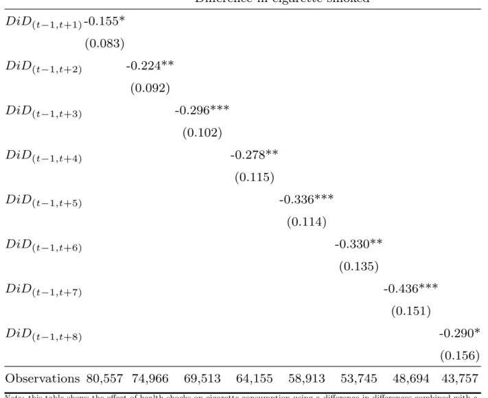
Table 2 shows the effect of a health shock on cigarette consumption using the difference-in-differences approach combined with a propensity score matching, as described in equation 7. We report results as follows. Column 1 gives the difference between the average number of cigarettes smoked one year after the shock and one year before the shock. Column 2 provides the same difference but 2 years after the shock. Likewise, columns 3 to 7 report

21_{SeeGoto et al.(2009);Fieulaine and Martinez(2010);Hall et al.(2012);Jusot and Khlat(2013)) for a}

the effect of health shocks from 3 to 7 years after the shock. Individuals facing shocks reduce their cigarette consumption by comparison with individuals who do not face such shocks. More precisely, individuals facing such shocks reduce their consumption, on average, by 2 cigarettes per week and this reduction seems to be become more important as time goes by. This could indicate that as ,addiction recedes, individuals are increasingly able to further reduce their cigarette consumption. This corroborates epidemiological findings showing that reducing cigarette consumption reduces dependency (McNeill(2004);Benowitz and Henningfield (2013); Begh et al.(2015)).

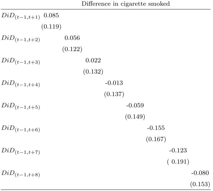
While facing a health shock reduces the number of cigarette smoked on average, signifi-cant disparities may exist in the population and need to be further documented. To study heterogeneous effects, we compare occasional and heavy smokers, the former being defined as smoking at most 5 cigarettes per day and the latter at least 15 cigarettes per day. The results (Table 3 and 4) show that heavy smokers are more likely to reduce their cigarette consumption, compared to occasional smokers, for whom no significant effect was found.

Our results are in line with other international studies. In the US, in the UK, and in Denmark heavy smokers are more likely to remain abstinent after trying to stop smoking than occasional smokers (Burns (2000);Godtfredsen et al. (2001); Kotz et al.(2012)). This may be because heavy smokers receive more advice from their GP than occasional smokers (Kotz et al.(2013)). Further, our findings contribute to a growing literature on the stability of health preferences (Craig et al. (2014); Ami et al. (2017); Bunn et al. (2006); Masanja et al. (2012)). Health preferences here refer to the individuals’ readiness to adopt healthy behaviors. Smokers could therefore be seen as individuals with low health preferences. If health preferences were stable over time, then smokers would not reduce their cigarette consumption after shocks. We observe the opposite, which may suggest individuals are not endowed with constant health preferences. Several explications could be offered to better understand this finding. First, the cost of smoking becomes more important for heavy smokers once the shock occurs. This finding is consistent with (Orphanides and Zervos

(1995))’s theoretical model suggesting that individuals learn from their own experience. Second, the impact of shocks could also contribute to modify time preferences (i.e. the degree to which one values the future more than the present) and/or risk preferences. Health shocks could lead to increase individuals’ preferences for the future, which is in line with

previous research on the impact of information campaigns on smoking patterns (Kenkel

(1991); Chaloupka and Wechsler (1997); Clark and Etil´e (2002)). Health shocks may also increase risk aversion, nudging individuals to be more cautious about their health.

4.2

Robustness checks

Two robustness checks were performed to assess the sensitivity of our results to the matching strategy, by testing alternative types of matching strategy.

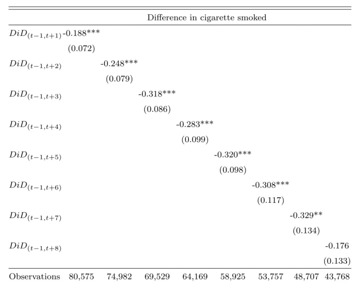
First, we use a radius matching approach (Dehejia and Wahba (2002)), which includes not only the nearest neighbors within the caliper, but also all comparison members within the caliper. Using a 0.5 radius, an individual in the treatment group is thus matched with all individuals in the control group with a propensity score within a 0.5 difference. By using all comparison individuals available within the radius, it extends the number of units when good matches are available, thereby reducing the risk of bad matches. Table 5 shows robust and significant results.

Second, we implement a Kernel matching (Heckman et al.(1997);Heckman et al.(1998)). This is a non-parametric matching estimator using weighted averages of all individuals in the control group to construct the counterfactual outcomes. In this case, an individual in the treatment group is matched with all individuals in the control group and control individuals who are closer to the treated individual are given higher weights. One major advantage of this approach is to lower the variance as more information is used. Further, to avoid bad matches, we only keep individuals belonging to the common support. Table 6 shows results in line with the propensity score matching.

Overall, our results are robust to these two alternative matching strategies, which indi-cates that the reduction in cigarette consumption could, thus, reasonably be attributed to the health shock experienced.

A further robustness check is carried out, comparing individuals who experience shocks at different times over the 25 years span. In order to take into account this heterogeneous situation, we split the group and run separate regressions for two subgroups: those who experience the shock before 1991 and those who experience it after 2004 (in Table 7). We find that the difference in cigarette smoked is higher for the first group. The fact that results differ across the two time periods is an indication of the existence of trend, with an

increasing level of information on tobacco toxicity. These findings validate the matching approach adopted in this paper.

5

CONCLUSION

The paper offers informative evidence on how French workers from the national Gaz and Electricity board have changed their tobacco intake following an acute health shock. The findings suggest that there is a significant effect running from the shock to the number of cigarettes smoked with impact duration of eight years after the shock. Individuals subject to a shock smoke on average 2 cigarettes less (per week) than those who did not face such a shock. Further, heavy smokers are more likely to reduce tobacco consumption than occa-sional smokers. More generally, our results suggest both that health shocks nudge individuals to change their health behaviors and that individuals do not seem to display stable health preferences.

Our results, nonetheless, face external and internal validity limitations. External limita-tion is related to the fact that the sample is not representative of the French populalimita-tion. We only have information for individuals working in the public sector and aged 36 to 75; Males are over represented (73,26%) by comparison to their general population share (48,41%). There are more blue collars in the Gazel data, compared to the French population (31% versus 12,8%)22_{. Internal validity limitation is due to unobserved heterogeneity. Individual}

preferences (i.e. risk and time preferences) are not observed, and are likely to influence both the probability of being treated, and of smoking. If these preferences are stable over time, the first differences of our DiD alleviates this problem. Further, we are not able to document the severity level in the health shock variable, and neither can we distinguish between traffic or work accident.

The policy implications of our research suggests designing information campaigns that are as close as possible to individuals’ own experiences, mimicking the effects of health shocks or relying on peers’ experience sharing. A possible illustration could be the campaign in Uruguay: pictures of newborn defects on cigarette packs will induce future mothers to quit smoking (Harris et al.(2015)). Likewise, our results seem to emphasize the fact that the time

at which information is released matters (in our case, after the shock). Indeed individuals may be more sensitive to preventive information once they experienced a negative health shock. Yet, the present analysis cannot inform as to the individual’s motivation behind the decision to reduce or stop smoking. To do so, detailed information on individuals’ preferences would be needed here, such as that collected on a regular basis in the innovation panel of the UK Understanding Society panel. This would help identify the precise pathways that influence these complex decisions.

References

Ag¨uero, J. M. and Beleche, T. (2017). Health shocks and their long-lasting impact on health behaviors: Evidence from the 2009 h1n1 pandemic in mexico. Journal of Health Economics, 54:40–55.

Ami, D., Aprahamian, F., and Luchini, S. (2017). Stated preferences and decision-making: Three applications to health. Revue ´economique, 68(3):327–333.

Bala, V. and Goyal, S. (1998). Learning from neighbours. The review of economic studies, 65(3):595–621.

Barnay, T., Halima, M. A. B., Duguet, E., Lanfranchi, J., and Le Clainche, C. (2015). La survenue du cancer: effets de court et moyen termes sur l’emploi, le chomage et les arrets maladie. Economie et statistique, 475(1):157–186.

Becker, G. S. and Murphy, K. M. (1988). A theory of rational addiction. Journal of political Economy, 96(4):675–700.

Begh, R., Lindson-Hawley, N., and Aveyard, P. (2015). Does reduced smoking if you can’t stop make any difference? BMC medicine, 13(1):257.

Benowitz, N. L. and Henningfield, J. E. (2013). Reducing the nicotine content to make cigarettes less addictive. Tobacco control, 22(suppl 1):i14–i17.

Bunn, H., Lange, I., Urrutia, M., Sylvia Campos, M., Campos, S., Jaimovich, S., Campos, C., Jacobsen, M. J., and Gaboury, I. (2006). Health preferences and decision-making needs of disadvantaged women. Journal of advanced nursing, 56(3):247–260.

Burns, D. M. (2000). Cigarette smoking among the elderly: disease consequences and the benefits of cessation. American Journal of Health Promotion, 14(6):357–361.

Byrnes, J. P., Miller, D. C., and Schafer, W. D. (1999). Gender differences in risk taking: A meta-analysis.

Callen, M., Isaqzadeh, M., Long, J. D., and Sprenger, C. forthcoming. violent trauma and risk preference: experimental evidence from afghanistan. American Economic Review.

Chaloupka, F. J. and Warner, K. E. (2000). The economics of smoking. Handbook of health economics, 1:1539–1627.

Chaloupka, F. J. and Wechsler, H. (1997). Price, tobacco control policies and smoking among young adults. Journal of health economics, 16(3):359–373.

Clark, A. and Etil´e, F. (2002). Do health changes affect smoking? evidence from british panel data. Journal of health economics, 21(4):533–562.

Craig, B. M., Reeve, B. B., Cella, D., Hays, R. D., Pickard, A. S., and Revicki, D. A. (2014). Demographic differences in health preferences in the united states. Medical care, 52(4):307. Daruvala, D. (2007). Gender, risk and stereotypes. Journal of Risk and Uncertainty,

35(3):265–283.

Decker, S. and Schmitz, H. (2016). Health shocks and risk aversion. Journal of health economics, 50:156–170.

Dehejia, R. H. and Wahba, S. (2002). Propensity score-matching methods for nonexperi-mental causal studies. The review of economics and statistics, 84(1):151–161.

Dom, G., Dhaene, P., Hulstijn, W., and Sabbe, B. (2006). Impulsivity in abstinent early-and late-onset alcoholics: differences in self-report measures and a discounting task. Addiction, 101(1):50–59.

Falba, T. (2005). Health events and the smoking cessation of middle aged americans. Journal of behavioral medicine, 28(1):21–33.

Fieulaine, N. and Martinez, F. (2010). Time under control: Time perspective and desire for control in substance use. Addictive Behaviors, 35(8):799–802.

Garcia-Gomez, P. (2011). Institutions, health shocks and labour market outcomes across europe. Journal of health economics, 30(1):200–213.

Garcia Gomez, P. and Lopez Nicola, A. (2006). Health shocks, employment and income in the spanish labour market. Health economics, 15(9):997–1009.

Garcia-Gomez, P., Van Kippersluis, H., O’Donnell, O., and Van Doorslaer, E. (2013). Long-term and spillover effects of health shocks on employment and income. Journal of Human Resources, 48(4):873–909.

Godtfredsen, N. S., Prescott, E., Osler, M., and Vestbo, J. (2001). Predictors of smoking reduction and cessation in a cohort of danish moderate and heavy smokers. Preventive medicine, 33(1):46–52.

Goldberg, M., Leclerc, A., Bonenfant, S., Chastang, J. F., Schmaus, A., Kaniewski, N., and Zins, M. (2006). Cohort profile: the gazel cohort study. International journal of epidemiology, 36(1):32–39.

Goto, R., Takahashi, Y., Nishimura, S., and Ida, T. (2009). A cohort study to exam-ine whether time and risk preference is related to smoking cessation success. Addiction, 104(6):1018–1024.

Grossman, M. (1972). On the concept of health capital and the demand for health. Journal of Political economy, 80(2):223–255.

Guiso, L. and Paiella, M. (2008). Risk aversion, wealth, and background risk. Journal of the European Economic association, 6(6):1109–1150.

Hall, P. A., Fong, G. T., Yong, H.-H., Sansone, G., Borland, R., and Siahpush, M. (2012). Do time perspective and sensation-seeking predict quitting activity among smokers? findings from the international tobacco control (itc) four country survey. Addictive behaviors, 37(12):1307–1313.

Harris, J. E., Balsa, A. I., and Triunfo, P. (2015). Tobacco control campaign in uruguay: Impact on smoking cessation during pregnancy and birth weight. Journal of health eco-nomics, 42:186–196.

Heckman, J. J., Ichimura, H., and Todd, P. (1998). Matching as an econometric evaluation estimator. The review of economic studies, 65(2):261–294.

Heckman, J. J., Ichimura, H., and Todd, P. E. (1997). Matching as an econometric evaluation estimator: Evidence from evaluating a job training programme. The review of economic studies, 64(4):605–654.

Heckman, J. J., LaLonde, R. J., and Smith, J. A. (1999). The economics and econometrics of active labor market programs. Handbook of labor economics, 3:1865–2097.

Imbens, G. W. and Wooldridge, J. M. (2009). Recent developments in the econometrics of program evaluation. Journal of economic literature, 47(1):5–86.

Jaroni, J. L., Wright, S. M., Lerman, C., and Epstein, L. H. (2004). Relationship between education and delay discounting in smokers. Addictive behaviors, 29(6):1171–1175. Jones, A. M. (1994). Health, addiction, social interaction and the decision to quit smoking.

Journal of health economics, 13(1):93–110.

Jones, A. M., Rice, N., and Zantomio, F. (2016). Acute health shocks and labour market outcomes.

Jusot, F. and Khlat, M. (2013). The role of time and risk preferences in smoking inequalities: a population-based study. Addictive behaviors, 38(5):2167–2173.

Keenan, P. S. (2009). Smoking and weight change after new health diagnoses in older adults. Archives of Internal Medicine, 169(3):237–242.

Kelly, M. M., Jensen, K. P., and Sofuoglu, M. (2015). Co-occurring tobacco use and posttrau-matic stress disorder: Smoking cessation treatment implications. The American journal on addictions, 24(8):695–704.

Kenkel, D. S. (1991). Health behavior, health knowledge, and schooling. Journal of Political Economy, 99(2):287–305.

Khwaja, A., Sloan, F., and Chung, S. (2006). The effects of spousal health on the deci-sion to smoke: Evidence on consumption externalities, altruism and learning within the household. Journal of Risk and Uncertainty, 32(1):17–35.

Kotz, D., Fidler, J., and West, R. (2012). Very low rate and light smokers: smoking patterns and cessation-related behaviour in england, 2006–11. Addiction, 107(5):995–1002.

Kotz, D., Willemsen, M. C., Brown, J., and West, R. (2013). Light smokers are less likely to receive advice to quit from their gp than moderate-to-heavy smokers: a comparison of

national survey data from the netherlands and england. The European journal of general practice, 19(2):99–105.

Lechner, M. et al. (2011). The estimation of causal effects by difference-in-difference methods. Foundations and Trends in Econometrics, 4(3):165–224.R

Malmendier, U. and Nagel, S. (2011). Depression babies: do macroeconomic experiences affect risk taking? The Quarterly Journal of Economics, 126(1):373–416.

Margolis, J., Hockenberry, J., Grossman, M., and Chou, S.-Y. (2014). Moral hazard and less invasive medical treatment for coronary artery disease: the case of cigarette smoking. Technical report, National Bureau of Economic Research.

Masanja, I. M., Lutambi, A. M., and Khatib, R. A. (2012). Do health workers’ preferences influence their practices? assessment of providers’ attitude and personal use of new treat-ment recommendations for managetreat-ment of uncomplicated malaria, tanzania. BMC Public Health, 12(1):956.

McNeill, A. (2004). Abc of smoking cessation: Harm reduction. BMJ: British Medical Journal, 328(7444):885.

Op den Velde, W., Aarts, P. G., Falger, P. R., Hovens, J. E., van Duijn, H., de Groen, J. H., and van Duijn, M. A. (2002). Alcohol use, cigarette consumption and chronic post-traumatic stress disorder. Alcohol and Alcoholism, 37(4):355–361.

Orphanides, A. and Zervos, D. (1995). Rational addiction with learning and regret. Journal of Political Economy, 103(4):739–758.

Richards, M. R. and Marti, J. (2014). Heterogeneity in the smoking response to health shocks by out-of-pocket spending risk. Health Economics, Policy and Law, 9(4):343–357. Riphahn, R. T. (1999). Income and employment effects of health shocks a test case for the

german welfare state. Journal of Population Economics, 12(3):363–389.

Sahm, C. R. (2012). How much does risk tolerance change? The quarterly journal of finance, 2(04):1250020.

Schmidt, L. (2008). Risk preferences and the timing of marriage and childbearing. Demog-raphy, 45(2):439–460.

Siegrist, M., Cvetkovich, G., and Gutscher, H. (2002). Risk preference predictions and gender stereotypes. Organizational Behavior and Human Decision Processes, 87(1):91–102. Sloan, F. A., Smith, V. K., and Taylor, D. H. (2003). The smoking puzzle: Information, risk

perception, and choice. Harvard University Press.

Smith, J. A. and Todd, P. E. (2005). Does matching overcome lalonde’s critique of nonex-perimental estimators? Journal of econometrics, 125(1):305–353.

Smith, V. K., Taylor Jr, D. H., Sloan, F. A., Johnson, F. R., and Desvousges, W. H. (2001). Do smokers respond to health shocks? The Review of Economics and Statistics, 83(4):675–687.

Sundmacher, L. (2012). The effect of health shocks on smoking and obesity. The European Journal of Health Economics, 13(4):451–460.

Trevisan, E. and Zantomio, F. (2016). The impact of acute health shocks on the labour supply of older workers: Evidence from sixteen european countries. Labour Economics, 43:171–185.

Wardle, J. and Steptoe, A. (2003). Socioeconomic differences in attitudes and beliefs about healthy lifestyles. Journal of Epidemiology & Community Health, 57(6):440–443.

Wooldridge, J. M. (2000). The initial conditions problem in dynamic, nonlinear panel data models with unobserved heterogeneity. University of Bristol, Department of Economics.

6

TABLES & FIGURES

Figure 1: Distribution of the propensity scores by groups before and after the matching.

.004 .005 .006 .007 .008 D e n si ty 19900 19950 20000 20050 Propensity scores before matching

Treated Control .004 .005 .006 .007 .008 D e n si ty 19900 19950 20000 20050 Propensity scores after matching

Treated Control

Note: this figure shows the distribution of the propensity scores and its density among the treated and the control group. It displays that before the matching there are some differences between these two groups. After the matching, however, the two groups seem to be more comparable. The distribution of the propensity score does not run from 0 to 1 as it is the result of the

Figure 2: Distribution of the propensity score among control and treatment groups. 0 2 4 6 8 D e n si ty .1 .2 .3 .4 .5 .6 Pr(individu_accident) Treated Control

Note: this figure displays that most of the treated individuals have a matched control with propensity score close to their own (most are less than a 0.005 differences).

Table 1: Achieved balancing on conditioning variables. Before matching After matching

Variables Treated Matched P-value Treated Matched % bias P-value

Father’s profession Farmer 0.107 0.105 0.877 0.107 0.094 4.2 0.374 Artisan 0.123 0.122 0.953 0.123 0.116 1.9 0.694 Executive or manager 0.216 0.223 0.594 0.216 0.240 -6.0 0.220 Intermediate profession 0.061 0.059 0.679 0.062 0.072 -4.3 0.398 Employee 0.297 0.321 0.136 0.297 0.302 -1.2 0.807 Worker 0.110 0.090 0.045 0.110 0.091 6.4 0.185 Educational attainment Higher degree 0.267 0.270 0.866 0.886 0.876 3.4 0.498 Marital status Couple 0.886 0.901 0.149 0.886 0.876 3.4 0.498 Divorced or separated 0.076 0.071 0.613 0.076 0.084 -3.3 0.508 Household income 6,5000 to less than 7,500 0.002 0.007 0.085 0.002 0.003 -1.4 0.704 7,500 to less than 9,000 0.022 0.032 0.112 0.022 0.015 5.0 0.207 9,000 to less than 10,500 0.085 0.098 0.199 0.085 0.088 -0.7 0.887 10,500 to less than 13,000 0.115 0.113 0.904 0.115 0.114 0.1 0.980 13,000 to less than 17,000 0.216 0.194 0.114 0.216 0.204 2.9 0.544 17,000 to less than 25,000 0.287 0.265 0.145 0.287 0.305 -4.1 0.402 25,000 and more 0.271 0.288 0.249 0.271 0.272 -0.3 0.943 Professional status Sick leave 0.009 0.006 0.299 0.009 0.007 2.4 0.625 Retired 0.349 0.267 0.000 0.349 0.342 1.4 0.782

Retired with professional activities 0.018 0.015 0.365 0.018 0.015 2.4 0.620

Cigarette smoked 13.564 14.012 0.258 13.564 14.067 -4.3 0.358 Self-reported health Very bad 0.254 0.273 0.212 0.254 0.261 -1.4 0.770 bad 0.344 0.314 0.057 0.344 0.319 5.4 0.263 Average 0.191 0.203 0.389 0.191 0.192 -0.2 0.968 Sufficient 0.103 0.106 0.814 0.103 0.114 -3.5 0.473 good 0.060 0.042 0.010 0.060 0.050 4.3 0.391 Very good 0.004 0.008 0.256 0.004 0.009 -5.8 0.247 Excelent 0.003 0.003 0.987 0.003 0.005 -3.3 0.547 Sexe 0.246 0.257 0.461 0.246 0.224 5.1 0.271 Age 53.196 53.451 0.219 53.196 53.107 1.5 0.760 Place of residence Big cities 0.324 0.312 0.426 0.324 0.342 -3.7 0.441 Suburb 0.066 0.084 0.059 0.066 0.085 -7.2 0.136 Isolated city 0.139 0.146 0.523 0.139 0.115 6.7 0.144 Alcohol consumption Occasional drinkers 0.479 0.459 0.224 0.479 0.493 -2.8 0.555 Frequent drinkers 0.218 0.237 0.180 0.218 0.235 -4.3 0.371 Heavy drinkers 0.113 0.126 0.263 0.113 0.116 -0.9 0.842

Note: This table reports the balancing between the two groups. There is no statistical differences between groups after matching. The standardised % bias is measured as the difference of the means in the treated and non-treated as a percentage of the square root of the average of

Table 2: Difference-in-differences with propensity score matching

Difference in cigarette smoked DiD_(t−1,t+1)-0.155* (0.083) DiD_(t−1,t+2) -0.224** (0.092) DiD_(t−1,t+3) -0.296*** (0.102) DiD_(t−1,t+4) -0.278** (0.115) DiD_(t−1,t+5) -0.336*** (0.114) DiD_(t−1,t+6) -0.330** (0.135) DiD_(t−1,t+7) -0.436*** (0.151) DiD_(t−1,t+8) -0.290* (0.156) Observations 80,557 74,966 69,513 64,155 58,913 53,745 48,694 43,757

Note: this table shows the effect of health shocks on cigarette consumption using a difference-in-differences combined with a propensity score matching. Individuals facing health shocks are more likely to reduce smoking. This effect lasts at least 8

Table 3: Heterogeneous effect:

Difference-in-differences with propensity score matching for occasional smokers

Difference in cigarette smoked

DiD

0.085

(0.119)

DiD

0.056

(0.122)

DiD

0.022

(0.132)

DiD

-0.013

(0.137)

DiD

-0.059

(0.149)

DiD

-0.155

(0.167)

DiD

-0.123

( 0.191)

DiD

-0.080

(0.153)

Observations 24,218 22,475 20,781 19,119 17,499 15,914 14,353 12,835

Note: this table shows the effect of health shocks on cigarette consumption using a difference-in-differences combined with a propensity score matching. Occasional smokers do not reduce their cigarette consumption after shocks. Standard deviations

Table 4: Heterogeneous effect:

Difference-in-differences with propensity score matching for heavy smokers

Difference in cigarette smoked DiD_(t−1,t+1)-0.315*** (0.132) DiD_(t−1,t+2) -0.452*** (0.144) DiD_(t−1,t+3) -0.559*** (0.161) DiD(t−1,t+4) -0.434*** (0.191) DiD_(t−1,t+5) -0.483** (0.188) DiD_(t−1,t+6) -0.475** (0.167) DiD_(t−1,t+7) -0.558** (0.258) DiD_(t−1,t+8) -0.459* (0.270) Observations 39,153 36,515 33,934 31,404 28,926 26,465 24,074 21,721

Note: this table shows the effect of health shocks on cigarette consumption using a difference-in-differences combined with a propensity score matching. Heavy smokers reduce their cigarette consumption after shocks. Standard deviations in

Table 5: Robustness checks:

Difference-in-differences with Radius matching

Difference in cigarette smoked

DiD_(t−1,t+1)-0.188*** (0.072) DiD_(t−1,t+2) -0.248*** (0.079) DiD_(t−1,t+3) -0.318*** (0.086) DiD_(t−1,t+4) -0.283*** (0.099) DiD_(t−1,t+5) -0.320*** (0.098) DiD_(t−1,t+6) -0.308*** (0.117) DiD_(t−1,t+7) -0.329** (0.134) DiD_(t−1,t+8) -0.176 (0.133) Observations 80,575 74,982 69,529 64,169 58,925 53,757 48,707 43,768

Note: this table shows robust coefficients of the effect of health shocks on cigarette consumption. Individuals facing health shocks are more likely to reduce smoking. Standard deviations in parentheses. * p < 0.05, ** p < 0.01, *** p < 0.001.

Table 6: Robustness checks:

Difference-in-differences with Kernel matching

Difference in cigarette smoked DiD_(t−1,t+1)-0.178** (0.072) DiD_(t−1,t+2) -0.237*** (0.079) DiD_(t−1,t+3) -0.307*** (0.087) DiD_(t−1,t+4) -0.269*** (0.098) DiD_(t−1,t+5) -0.306*** (0.098) DiD_(t−1,t+6) -0.291** (0.117) DiD_(t−1,t+7) -0.316** (0.134) DiD_(t−1,t+8) -0.166 (0.133) Observations 80,575 74,982 69,529 64,169 58,925 53,757 48,707 43,768

Note: this table shows robust coefficients of the effect of health shocks on cigarette consumption. Individuals facing health shocks are more likely to reduce smoking. Standard deviations in parentheses. * p < 0.05, ** p < 0.01, *** p < 0.001.

Table 7: Heterogeneous effect of health shocks: Differences between groups before 1991 and after 2004

Difference in cigarette smoked

Difference in cigarette smoked

Before 1991

After 2004

DiD

-0.694*

-0.172*

(0.391)

(0.102)

Observations

5,497

43,237

Note: This table reports heterogeneous effect of cigarette consumption between groups depending on time horizon. Individuals living in the beginning of the 90’s are less likely to be exposed to long and continous preventive (and information) campaings than individuals living after 2004. Therefore, the later could benefit from those policies which help them to reduce