Temporal and spatial structure of multi-millennial temperature changes at high latitudes during the Last Interglacial

(1)

HAL Id: hal-02180978

https://hal.archives-ouvertes.fr/hal-02180978

Submitted on 11 Jul 2019

HAL is a multi-disciplinary open access

archive for the deposit and dissemination of

sci-entific research documents, whether they are

pub-lished or not. The documents may come from

teaching and research institutions in France or

abroad, or from public or private research centers.

L’archive ouverte pluridisciplinaire HAL, est

destinée au dépôt et à la diffusion de documents

scientifiques de niveau recherche, publiés ou non,

émanant des établissements d’enseignement et de

recherche français ou étrangers, des laboratoires

publics ou privés.

Temporal and spatial structure of multi-millennial

temperature changes at high latitudes during the Last

Interglacial

Émilie Capron, Aline Govin, Emma Stone, Valérie Masson-Delmotte, Stefan

Mulitza, Bette L. Otto-Bliesner, Tine L. Rasmussen, Louise C. Sime, Claire

Waelbroeck, Eric W. Wolff

To cite this version:

Émilie Capron, Aline Govin, Emma Stone, Valérie Masson-Delmotte, Stefan Mulitza, et al..

Temporal and spatial structure of multi-millennial temperature changes at high latitudes

dur-ing the Last Interglacial.

Quaternary Science Reviews, Elsevier, 2014, 103, pp.116-133.

(2)

Temporal and spatial structure of multi-millennial temperature

changes at high latitudes during the Last Interglacial

Emilie Capron

a,*

_{, Aline Govin}

b

_{, Emma J. Stone}

c

_{, Val!erie Masson-Delmotte}

d

_,

Stefan Mulitza

b

_{, Bette Otto-Bliesner}

e

_{, Tine L. Rasmussen}

f

_{, Louise C. Sime}

a

_,

Claire Waelbroeck

d

, Eric W. Wolff

g

a_{British Antarctic Survey, High Cross, Madingley Road, CB3 0ET Cambridge, UK}

b_{MARUM/Center for Marine Environmental Sciences, University of Bremen, Leobener Strasse, 28359 Bremen, Germany} c_{BRIDGE, School of Geographical Sciences, University of Bristol, Bristol BS8 1SS, UK}

d_{Institut Pierre-Simon Laplace/Laboratoire des Sciences du Climat et de l'Environnement, UMR 8212, CEA-CNRS-UVSQ, 91191 Gif-sur-Yvette, France} e_{Climate and Global Dynamics Division, National Center for Atmospheric Research (NCAR), Boulder, CO 80305, USA}

f_{CAGE-Centre for Arctic Gas Hydrate, Environment and Climate, UiT, the Arctic University of Norway, Tromsø, Norway} g_{Godwin Laboratory for Palaeoclimate Research, Department of Earth Sciences, University of Cambridge, CB2 3EQ Cambridge, UK}

a r t i c l e i n f o

Article history: Received 31 March 2014 Received in revised form 20 August 2014 Accepted 22 August 2014 Available online Keywords:

Last Interglacial period Marine sediment cores Ice cores

Data synthesis

Climate model simulations

a b s t r a c t

The Last Interglacial (LIG, 129e116 thousand of years BP, ka) represents a test bed for climate model feedbacks in warmer-than-present high latitude regions. However, mainly because aligning different palaeoclimatic archives and from different parts of the world is not trivial, a spatio-temporal picture of LIG temperature changes is difﬁcult to obtain.

Here, we have selected 47 polar ice core and sub-polar marine sediment records and developed a strategy to align them onto the recent AICC2012 ice core chronology. We provide the ﬁrst compilation of high-latitude temperature changes across the LIG associated with a coherent temporal framework built between ice core and marine sediment records. Our new data synthesis highlights non-synchronous maximum temperature changes between the two hemispheres with the Southern Ocean and Antarctica records showing an early warming compared to North Atlantic records. We also observe warmer than present-day conditions that occur for a longer time period in southern high latitudes than in northern high latitudes. Finally, the amplitude of temperature changes at high northern latitudes is larger compared to high southern latitude temperature changes recorded at the onset and the demise of the LIG.

We have also compiled four data-based time slices with temperature anomalies (compared to present-day conditions) at 115 ka, 120 ka, 125 ka and 130 ka and quantitatively estimated temperature un-certainties that include relative dating errors. This provides an improved benchmark for performing more robust model-data comparison. The surface temperature simulated by two General Circulation Models (CCSM3 and HadCM3) for 130 ka and 125 ka is compared to the corresponding time slice data synthesis. This comparison shows that the models predict warmer than present conditions earlier than documented in the North Atlantic, while neither model is able to produce the reconstructed early Southern Ocean and Antarctic warming. Our results highlight the importance of producing a sequence of time slices rather than one single time slice averaging the LIG climate conditions.

1. Introduction

Due to numerous positive feedbacks, polar regions act as am-pliﬁers of climate change (e.g. CAPE Last Interglacial Project

Members, 2006; Masson-Delmotte et al., 2013; Nikolova et al., 2013). During the last decade, the Arctic has experienced the strongest warming trend observed at the Earth's surface, and further climate change is expected to produce large environmental changes in the near future including Arctic glaciers and Greenland ice sheet contributions to projected sea level rise (Church et al., 2013). By contrast, recent sea ice and temperature trends in and around Antarctica appear more complex, and this area is expected

*Corresponding author. Tel.: þ44 1223 221 368; fax: þ44 1223 362 616. E-mail address:ecap@bas.ac.uk(E. Capron).

Contents lists available atScienceDirect

Quaternary Science Reviews

j o u r n a l h o m e p a g e : w w w . e l s e v i e r . c o m / l o c a t e / q u a s c i r e v

http://dx.doi.org/10.1016/j.quascirev.2014.08.018

(3)

to respond on longer time scales to increased greenhouse gas emissions, with large uncertainties on associated sea level risks. The ability of climate models to correctly capture feedbacks involved in polar ampliﬁcation remains uncertain and past climatic changes provide benchmarks against which the realism of climate models can be assessed (Braconnot et al., 2012; Schmidt et al., 2014). In particular, studying past warm periods such as recent interglacial periods, provide unique insights to assess polar ampliﬁcation feedbacks in a range of temperature changes com-parable to projected future changes (e.g.Otto-Bliesner et al., 2013). The Last Interglacial period (hereafter LIG; 129e116 thousand of years BP, hereafter ka) is of particular interest since large parts of the globe were characterised by a warmer-than-present day climate (e.g. CAPE Last Interglacial Project Members, 2006; Turney and Jones, 2010). While orbital insolation was distinctly different to present-day (Laskar et al., 2004), atmospheric CO2concentration

levels were close to pre-industrial values (Lüthi et al., 2008). The LIG is not an analogue for future climate change because orbital forcing is fundamentally different from anthropogenic forcing, and because the geographical pattern of LIG temperature changes strongly differ from those expected in the future (Masson-Delmotte et al., 2011a). Nonetheless, it offers an opportunity to assess the effect of warmer-than-present-day polar climate on climate-sensitive parts of the Earth system, most notably polar ice sheets and sea level. Previous work suggests that global sea level was 5.5e9 m higher than today (e.g.Kopp et al., 2009; Thompson et al., 2011). Combined with earlier evidence for LIG ice at the bottom of the Greenland ice sheet (e.g.

GRIP members, 1993), the NEEM ice core data demonstrate the resilience of the central Greenland ice sheet to LIG local warming (NEEM community members, 2013). Ice sheet simulations compatible with NEEM elevation estimates suggest that the Greenland ice sheet contribution to the sea level rise should be in the range of 1.4e4.3 m (Robinson et al., 2011; Born and Nisancioglu, 2012; Masson-Delmotte et al., 2013; Quiquet et al., 2013; Stone et al., 2013). However, different input climates arising from climate simulations have been used as inputs for these ice sheet simulations. Also, the study of the LIG beneﬁts from numerous snapshot and transient climatic simulations with state of the art General Circula-tion Models (GCMs; e.g. Bakker et al., 2013; Lunt et al., 2013; Nikolova et al., 2013; Otto-Bliesner et al., 2013; Langebroek and Nisancioglu, 2014; Paleoclimate Modelling Intercomparison Project,

http://pmip3.lsce.ipsl.fr/). Altogether, this further motivates the evaluation of these GCMs against LIG climate reconstructions. In particular, data syntheses are required to document the magnitude and spatio-temporal structure of LIG temperature changes.

Several climatic data compilation initiatives have been con-ducted for the LIG (CLIMAP, 1984; Kaspar et al., 2005; CAPE Last Interglacial Project Members, 2006; Clark and Huybers, 2009; Turney and Jones, 2010; McKay et al., 2011). Turney and Jones (2010)averaged temperature estimates across the benthic forami-nifera

d

18O and ice

d

18O plateau in marine and ice core records respectively, and across the period of maximum warmth in terrestrial sequences. They deduced a global annual LIG “maximum” warming above pre-industrial of about 2"_{C and they}

identiﬁed earlier warming in Antarctica.McKay et al. (2011)used an alternative temperature-averaging method and calculated the mean sea surface temperature (SST) over a 5 ka period centred on the warmest temperature observed between 135 ka and 118 ka in marine records. They estimated a global annual mean SST warming of þ0.7 ± 0.6"_{C relative to the late Holocene.}

Otto-Bliesner et al. (2013)used these existing LIG temperature compilations to benchmark snapshot simulations performed at 125 and 130 ka with the CCSM3 GCM. However, both time slices are compared to a single data synthesis built assuming explicitly syn-chronous peak warmth. Recently,Bakker et al. (2014)proposed a

comparison of temperature rates of change inferred from transient simulations as well as sea surface temperature (SST) from alkenone data and polar temperature syntheses, albeit without common chronologies. Both studies stress uncertainties associated with chronologies and temperature-averaging procedures. A temporal description of the LIG climate rather than an asynchronous compilation of LIG temperature optima could allow a detailed evaluation of these model simulations.

Indeed, current temporal representations inferred from marine sediment and ice core records remain limited so far by the lack of a common robust age scale over the LIG. Existing LIG syntheses are currently based on records taken on their original timescale, introducing absolute dating uncertainties that can reach several thousand years (e.g. Waelbroeck et al., 2008; Bazin et al., 2013; Veres et al., 2013). However, there is evidence that surface tem-perature peaks are not globally coincident. In particular, there is a signiﬁcant delay in the establishment of peak interglacial condi-tions in the North Atlantic and Nordic Seas as compared to the Southern Ocean (Cortijo et al., 1999; Bauch and Erlenkeuser, 2008; Bauch et al., 2011; Van Nieuwenhove et al., 2011; Govin et al., 2012). Also, an early Antarctic warming has been reported ( Masson-Delmotte et al., 2010). Thus, a compilation with a dynamic repre-sentation of the sequence of climatic events (several time slices) taking into account potential asynchronous temperature changes between the two hemispheres during the LIG is necessary. This requires synchronising palaeoclimatic records from different ar-chives (e.g. ice cores and marine sediments).

The objectives of this study are twofold. First we document the magnitude and spatio-temporal structure of LIG temperature changes in the high latitudes of the two hemispheres. For that purpose, we describe a new data synthesis of air and sea surface temperature changes across the LIG in polar and sub polar regions associated with a coherent temporal framework between ice core and marine sediment records. Second, based on this new high latitude data compilation, we produce four data-based surface temperature anomaly time slices at 115 ka, 120 ka, 125 ka and 130 ka for which we propagate relative dating uncertainties and reconstructed temperature errors into the ﬁnal temperature anomaly estimates. Using snapshot simulations performed for the 125 ka and 130 ka climatic conditions by the CCSM3 and HadCM3 models, we illustrate how these new time slices enable more robust model-data comparison to be performed in order to test state-of-the-art GCMs also used to perform future climate projections. 2. Material and methods

2.1. Palaeoclimatic data selection

We selected sites presenting a mean time-resolution of tem-perature reconstruction better than 2 ka and sufﬁcient additional information (e.g. benthic and/or planktic

d

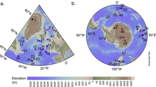
18O records, ash layers) to help integrate them with conﬁdence into the common temporal framework. We selected ﬁve records of surface air temperature deduced from water stable isotopes measured along polar ice cores and 42 SST records from marine sediment cores located above 40"_N

and 40"_{S of latitude (}_{Fig. 1}_{). We obtained data through the}

PAN-GAEA database, from individual papers provided by principal in-vestigators or extracted from published ﬁgures through digital image processing. Details for each selected record are given in

Table A1.

# Ice core records:

We include local surface air temperature reconstructions for the East Antarctic EPICA Dome C (EDC), EPICA Dronning Maud Land

(4)

(EDML), Vostok and Dome F ice cores based on the stable isotopic composition of the ice (Masson-Delmotte et al., 2011band references therein). Reconstructions of local surface temperature in Antarctic ice cores are based on the present day spatial relationship between the ice isotopic composition of the snow and surface temperature (“iso-topic thermometer”). While in principle they should reﬂect precipitation-weighted temperatures, they are considered here as annual means. Precipitation intermittency, changes in moisture origin as well as site elevation and ice origin changes (Jouzel et al., 2003; Masson-Delmotte et al., 2006; Vinther et al., 2009; Stenni et al., 2010) affect the quantiﬁed temperature changes from ice cores. In particular, a modelling study of projected climate and precipitation isotopic composition suggests that using such a method could result in an underestimation of past temperatures for periods warmer than present day conditions (Sime et al., 2009). It results in an uncertainty associated with the different ice-core-based Antarctic absolute tem-perature reconstructions from ±1"_{C to ±2}"_{C (}_{Stenni et al., 2010;}

Masson-Delmotte et al., 2011b).

Ice cores retrieved in Greenland are deﬁcient in providing a continuous or/and complete record of the LIG (GRIP members,1993; Grootes et al.,1993; NorthGRIP community members, 2004; NEEM c. m. 2013). Here, we use the NGRIP

d

18Oicefor record alignment

pur-poses between 123 and 110 ka as it represents the only continuous Greenlandic record covering this time interval. In Greenland, iso-topeetemperature relationships vary through time and have smaller slopes than the modern spatial gradient. We use here the precipitation-weighted temperature estimate corrected for eleva-tion and upstream effects deduced from the NEEM ice core between 116 and 128 ka (NEEM c. m., 2013). Note that while elevation effects are commonly considered to be negligible for Antarctic ice cores (Bradley et al., 2012, 2013), this is not the case for Greenland.

# Marine sediment cores:

The marine sediment records included in our data synthesis are mostly located in the North Atlantic region for the Northern Hemisphere and in the Indian and Atlantic sectors of the Southern Ocean for the Southern Hemisphere. The coverage of selected sites reﬂects the lack of high-resolution SST records covering the LIG in other high-latitude regions and emphasises the need for obtaining future SST records in particular in the Paciﬁc Ocean. SST

reconstructions are based on foraminiferal Mg/Ca ratios (three re-cords), alkenone unsaturation ratios (three records) and faunal assemblage transfer functions (24 records based on foraminifera assemblages, two records based on radiolarian assemblages and four records based on diatom assemblages) and the percentage of the polar foraminifera species Neogloboquadrina pachyderma sinistral (six records) (Fig. 1,Table A1). Therefore, our data compi-lation mostly includes SST reconstructions based on faunal as-semblages, which reﬂects the low amount of high-resolution SST records produced with alternative geochemical methods (e.g. alkenone paleothermometry, foraminiferal Mg/Ca) throughout the LIG.

We use these records as representing annual or summer SST as given by the authors of the respective papers. Note that in the case of core MD97-2121, both summer SST (record [27] onFig. 1and

Table A1, hereafter records are only designated such as [27]) and annual mean SST [28] have been reconstructed from the same source data while for core SU90-08 a summer SST record has been deduced from foraminifera assemblages ([23];Cortijo, 1995) and an annual SST record has been deduced based on alkenone paleo-thermometry ([22];Villanueva et al., 1998). Uncertainties on each reconstructed SST record were estimated from (1) the uncertainty on measurement and (2) the calibration of geochemical and microfossil proxies against modern conditions and range between 0.6 and 2.1"_{C depending on the SST proxies (uncertainties for}

in-dividual records are given inTable A1).

2.2. Strategy for aligning climatic records over the Last Interglacial Beyond the applicable range of radiocarbon dating, LIG re-constructions beneﬁt from few absolute markers. Large discrep-ancies of up to several thousand years exist between time scales used to display marine sediment cores and ice core timescales. As an example,Parrenin et al. (2007) report a 2 ka age difference across this time period between the LR04 time scale classically taken as a reference chronology to establish age models of marine sediment cores (Lisiecki and Raymo, 2005) and the EDC3 ice core chronology. Thus, the construction of a common chronostratig-raphy between ice core and marine records is critical to compare the LIG climate evolution in both the Northern and Southern Hemispheres.

Fig. 1. Location of marine sediment and ice core sites in a. the Northern Hemisphere and b. the Southern Hemisphere included in this study. The compilation contains surface air temperature records from Greenland (black square) and Antarctic (red square) ice cores and SST reconstructions (diamond) based on Mg/Ca (blue), alkenones (grey), diatoms assemblages (orange), radiolarians (green) and foraminifera assemblages (MAT method, purple; NPS percentage, pink). Numbers refer to record labels indicated inTable A1from the Appendix. (For interpretation of the references to colour in this ﬁgure legend, the reader is referred to the web version of this article.)

E. Capron et al. / Quaternary Science Reviews 103 (2014) 116e133 118

(5)

2.2.1. AICC2012, a new ice core dating and a reference chronology We use the new AICC2012 ice core chronology (Bazin et al., 2013; Veres et al., 2013) as a reference chronology to display the selected marine sediment and ice core records. The AICC2012 chronology is the ﬁrst integrated timescale over the LIG, based on a multi-site approach including both Greenland (NGRIP) and Ant-arctic ice cores (EDC, EDML, TALDICE, Vostok). The new chronology shows only small differences, well within the original uncertainty range, when compared with the EDC3 age scale over the LIG. However, the numerous new stratigraphic links signiﬁcantly reduce the absolute dating uncertainty down to ±1.6 ka (1

s

) over the LIG (Bazin et al., 2013) making it the most appropriate age scale to date with which to compare our synchronised records with model runs and other dated records.

The Dome F and the NEEM ice cores have not been included to construct the AICC2012 chronology (Bazin et al., 2013; Veres et al., 2013). However, both the Dome F and the NEEM ice cores have been previously transferred onto the EDC3 timescale (Parrenin et al., 2007; NEEM c. m., 2013). Thus by using published EDC3-AICC2012 age relationships (Bazin et al., 2013; Veres et al., 2013), we transfer the temperature records from the Dome F and the NEEM ice cores onto the AICC2012 chronology.

2.2.2. Transfer of marine records onto AICC2012

We follow the strategy ofGovin et al. (2012)to align marine records onto the AICC2012 ice core chronology. It is based on the assumption that surface-water temperature changes in the sub-Antarctic zone of the Southern Ocean (respectively in the North Atlantic) occurred simultaneously with air temperature variations over inland Antarctica (respectively Greenland). Such a link be-tween air above the polar ice sheets and surrounding surface wa-ters has been observed during the abrupt climate changes over the Last Glacial period and during Termination I which beneﬁt from robust radiocarbon dating constraints (Bond et al., 1993; Calvo et al., 2007). For instance, SST changes at site NA87-22 (14C-dated record, Waelbroeck et al., 2008, 2011) are synchronous within dating uncertainties with both the NorthGRIP

d

18Oice and CH4

concentration changes over the last 25 ka (Fig. 1 from Masson-Delmotte et al., 2010).

Benthic foraminiferal

d

18O is often used as a stratigraphic tool to place marine records on a common age model (e.g.Lisiecki and Raymo, 2005). We prefer avoiding using this strategy for all the selected marine records since there is evidence for signiﬁcant off-sets (from 1 ka to up to 4 ka) between benthic

d

18O records from different water masses and oceanic basins during deglaciations (e.g.

Skinner and Shackleton, 2005; Lisiecki and Raymo, 2009). However, no clear benthic

d

18O offsets (within dating uncertainties, ~2 ka) are observed during the penultimate deglaciation between North Atlantic sites located at different water-depth within the same North Atlantic Deep Water mass (Govin et al., 2012). Therefore, we use benthic foraminiferal

d

18O records to verify the overall agree-ment of chronologies deﬁned in North Atlantic or Southern Ocean sites located in the same water mass. For this purpose, we use cores MD02-2488 [38] and ODP980 [14] as Southern Ocean and North Atlantic references, respectively, because of the high temporal resolution of their SST records and the availability of multi-proxy records (i.e. planktic and benthic foraminiferal stable isotopes).

To align marine sediment cores onto the AICC2012 chronology, we use the software AnalySeries 2.0 (Paillard et al., 1996) and deﬁne the minimum number of tie points which produces the best possible alignment. Age models are constructed by linear interpo-lation (i.e. constant sedimentation rate) between tie-points. The relative uncertainty attached to each tie point is graphically esti-mated through multiple alignment possibilities. It takes into ac-count the time resolution of the records used to perform the

alignment and reflects how robust the tie-point is regarding its location (e.g. situated at the mid-point of a well-marked transition) and how synchronous the records used for the alignment become after defining the tie-point. A list of defined tie-points, corre-sponding rationale and relative 1

s

age uncertainties on the AICC2012 timescale is given for every selected sediment core in

Table A2.

# Southern Ocean cores: We align each SST record from the Southern Ocean onto the EDC deuterium record (

d

D,Jouzel et al.,

2007; site [45] onFig. 1) displayed on AICC2012. Our decision to align marine cores from all Southern Ocean sectors onto the EDC record is justiﬁed by the fact that the Dome F, EDML and EDC water stable isotope records show similar variations, with approximately simultaneous climatic transitions ( Masson-Delmotte et al., 2011b). Also considering either the EDC

d

D re-cord or the EDC site temperature estimate as a reference curve for aligning marine sediment records onto AICC2012 does not affect the timing of the glacial inception and the start of Termination II (Masson-Delmotte et al., 2011b). Termination II is slightly more abrupt in the site temperature record than in the

d

D record but it only leads to an age difference for the two corresponding mid slope points of less than 500 years.

Fig. 2(left panel) illustrates the alignment of core MD88-769 [37] onto AICC2012 based on four tie points. We define a first tie point by aligning the first SST increase with the EDC

d

D increase at the beginning of Termination II (138.2 ± 2 ka). Then, we deﬁne a mid-slope tie point in the course of the glacialeinterglacial tran-sition (131.4 ± 1 ka) and another mid-slope tie point during the glacial inception (116 ± 1.5 ka). Finally, a last relative age constraint is determined by tying the mid-slope of the

d

D increase corre-sponding to the Antarctic Isotopic Maxima 24 and its counterpart identiﬁed in the SST record (106.7 ± 2 ka). We are conﬁdent in our alignment since it results in simultaneous benthic

d

18O variations recorded in cores MD88-769 and MD02-2488 [38] (which was retrieved at a similar water depth and previously transferred onto AICC2012 following a similar strategy) (Fig. 2, left panel).

# North Atlantic cores: We align the SST proxy records from the North Atlantic cores to the ice

d

18O record from the NGRIP Greenland ice core during the Last Glacial inception. We favour the NGRIP ice core to the NEEM ice core as the Greenland reference ice core because (1) the NGRIP ice core is one of the ice records used to constrain the AICC2012 chronology and (2) the NGRIP ice core represents a continuous record up to 123 ka (NorthGRIP c. m. 2004) while the NEEM ice core record presents stratigraphic discontinuities at the end of the LIG (NEEM c. m. 2013). Since the NGRIP ice core does not cover the early LIG, alternative strategies are followed to align marine and ice core records prior to 122 ka. First, we assume that the global abrupt methane increase during Termination II reflects synchronous abrupt warming of the air above Greenland. This is indeed observed during Termination I as well as during millennial-scale DansgaardeOeschger events (e.g.Chappellaz et al., 1993; Huber et al., 2006; Baumgartner et al., 2013). OnFig. 2, the right panel illustrates the alignment of core SU90-44 [19] onto AICC2012 using four tie-points. The beginning of the LIG is relatively well constrained in all North Atlantic cores with a tie point linking the final SST increase with the abrupt methane increase recor-ded in the EDC ice core (128.7 ± 0.5 ka). However, in order to constrain the 130 ka time slice, it is necessary to define a tie point prior to 131 ka (see Section2.3). Thus, we define a first tie point during the preceding glacial period using the assumption that the establishment of the very cold glacial conditions related

(6)

to Heinrich event 11 is synchronous within the North Atlantic region. As a result, we tie the increase of the percentage of N. pachydermasinistral in core SU90-44 with the one recorded at 133.8 ± 2 ka in core ODP980 previously transferred onto AICC2012 (Table A2). Then, at the end of the LIG, the first pro-nounced North Atlantic cooling is tied to the corresponding enhanced cooling in the NGRIP ice core (116.8 ± 1.5 ka). We finally define a tie point that links SST and Greenland air tem-perature at the end of the first abrupt event, Dans-gaardeOeschger 25 (107.3 ± 1.5 ka). We are confident in the choice of these tie points since they lead to simultaneous in-creases in the percentage of N. pachyderma sinistral recorded in cores SU90-44 and ODP980 (Fig. 2, right panel). A similar pro-cedure is followed for all other North Atlantic high latitude sites except for the site EW9302-JPC2 [21] located in the Labrador Sea and for which it is less straightforward to define the alignment

onto AICC2012. Note that in the rest of the manuscript, we differentiate the North Atlantic high latitude region from the Labrador Sea area.

# Nordic Seas and Labrador Sea cores: Climatic alignments of re-cords retrieved in the Labrador Sea and the Nordic Seas are more equivocal for two main reasons. First, most of the SST estimates have been derived from the percentage of N. pachyderma sinistral which is not suitable to record SST variations below 6.5"_{C (}_{Tolderlund and Be, 1971; Kohfeld et al., 1996}_{). Indeed,}

while the percentage of this species is linearly related to SST changes for water of ~6.5e15 "_{C, the abundance of}

N. pachyderma sinistral already accounts for ~95% of forami-nifera faunal assemblages at 6.5 "_{C, thus any temperature}

change below this value cannot be tracked with this method (Kohfeld et al., 1996; Govin et al., 2012). Also, potential issues in the preservation of the planktic foraminifera shells may affect

Fig. 2. Deﬁnition of age models in the Southern Ocean MD88-769 core [34] (red curves) and the North Atlantic SU90-44 core [17] (blue curves). Numbers between brackets correspond to of the core location onFig. 1. Triangles (with error bars representing associated relative 1sdating uncertainties) and vertical dotted lines highlight the tie-points deﬁned between (left panel) the MD88-769 Summer SST record and the Antarctic EDCdD record (Jouzel et al., 2007; black) and (right panel) between the SU90-44 Summer SST record and the NGRIP iced18O record (NorthGRIP c. m. 2004; black), the CH4concentration measured in the air trapped in the EDC ice core (Loulergue et al., 2008; grey) and the

percentages of N. pachyderma sinistral (LSCE database). The resulting agreement between Summer SST and benthicd18O records from MD88-769 and MD02-2488 (Govin et al., 2012; grey) both displayed on AICC2012 is shown as well as resulting sedimentation rate variations and associated relative age uncertainty of the tie points for each core. Grey shaded areas mark non-parametric 2s(2.5th and 97.5th percentiles) conﬁdence intervals of Monte Carlo iterations (see text for details). (For interpretation of the references to colour in this ﬁgure legend, the reader is referred to the web version of this article.)

(7)

the SST reconstructions (e.g.Zamelczyk et al., 2012). Unfortu-nately to our knowledge, there are very few alternative quan-titative SST estimates available for the LIG in the Labrador Sea (only [11], [12], [13] and [21]) and in the Nordic Seas (only [7]) based on alternative SST reconstruction methods.

Second, planktic and benthic foraminiferal

d

18O are charac-terised by highly depleted

d

18O values during Termination II (e.g.

Risebrobakken et al., 2006; Bauch and Erlenkeuser, 2008), which makes the identiﬁcation of the LIG climatic optimum in forami-niferal stable isotopes difﬁcult. Very low benthic

d

18O during Termination II may derive from intensiﬁed sea ice formation and brine rejection that transferred to bottom waters the low

d

18O signal recorded in surface waters in response to strong iceberg melting (e.g.Risebrobakken et al., 2006). Alternatively,Bauch and Bauch (2001) proposed that such low benthic

d

18O values may reflect the warming of bottom waters in response to the inflow of warm subsurface Atlantic waters below fresh and stratified surface waters in the Nordic Seas.

To overcome these difﬁculties, we combine here several lines of evidence (i.e. temperature variations, tephra layers, foraminiferal stable isotopes, biostratigraphic constraints) to deﬁne chronolo-gies as robust as possible in the Norwegian and Labrador Seas. The

difficulty of performing these alignments is reflected in the rela-tively high relative dating uncertainties associated to each tie point (Table A2). In three of these high northern latitude sites, temperature anomalies cannot be reconstructed for the 130 and 115 ka data-based time slices due to the lack of chronological constraints. We update the chronology that was originally defined in the Labrador Sea core EW9302-JPC2 using the EDC3 timescale as a reference byGovin et al. (2012)in order to transfer the re-cords onto AICC2012. Fig. 3 illustrates how we transfer MD95-2009 [7] and HM71-19 [2] records from the Nordic Seas onto the AICC2012 chronology. First, the North Atlantic core ENAM33 [8] is transferred onto AICC2012 via the alignment of its SST record (Rasmussen et al., 2003; this study; Details are given on the SST reconstruction method in theappendix) to the NGRIP

d

18Oiceand

the EDC CH4concentration (see previous section for details on the

approach). Second, we deﬁne stratigraphic links between core ENAM33 and the Nordic sea core MD95-2009 to transfer the latter onto AICC2012. A ﬁrst tie point is determined based on the alignment of MD95-2009 benthic

d

18O record with core ODP980 at 138.2 ka associated with a relative age uncertainty of 4 ka. Such a relative age uncertainty takes into account the difﬁculty in deﬁning the tie point and the possible time lags between two benthic

d

18O records from different oceanic basins. Then, we

Fig. 3. Definition of age models in one North Atlantic (ENAM33 [8], green curves) and two Norwegian Sea sediment cores (MD95-2009 [7] and HM71-19 [2]). Numbers between brackets correspond to the location of records onFig. 1. ENAM33 core has been first transferred onto AICC2012 through climatic alignments (tie points indicated in black triangles). In addition to climatic alignment-based tie points (black triangles and pink square for the tie point proposed byRasmussen et al., 2003), core MD95-2009 was linked to core ENAM33 thanks to the ash layer Low/bas-IV identified in both cores (orange dot). Core HM71-19 was aligned onto core MD95-2009 based on the ash layers Midt/RHY and 5e-Low/bas-IV identified in both cores (orange dots) and planktic and benthicd18O records (black triangles). Sedimentation rate variations and defined relative age uncertainty are also shown for each core. Grey shaded areas mark non-parametric 2s(2.5th and 97.5th percentiles) confidence intervals of Monte Carlo iterations (see text for details). (For inter-pretation of the references to colour in this figure legend, the reader is referred to the web version of this article.)

(8)

(9)

include the biostratigraphic link proposed by Rasmussen et al. (2003) between cores MD95-2009 and ENAM33 dated at 128.0 ± 1.5 ka on AICC2012. These authors aligned in both cores the disappearance of Atlantic benthic foraminifera species groups that are replaced by benthic species associated with the cold Norwegian Sea Overflow Water, hereby reflecting the onset of convection in the Nordic seas (Rasmussen et al., 2003). We use also as a stratigraphic link the ash layer 5e-Low/BasIV identified in both ENAM33 and MD95-2009 cores (Rasmussen et al., 2003). While an older age was reported byRasmussen et al. (2003)based on a correlation onto the SPECMAP time scale, the ash layer 5e-Low/BasIV in core ENAM33 corresponds to a depth level dated at 123.7 ± 2 ka based on the deptheage relationship resulting from the alignment of this core onto AICC2012 (Fig. 3, left panel). Thus, this age of 123.7 ± 2 ka is used as a third tie point to constrain the age model of core MD95-2009 (Fig. 3, middle panel). At the end of the LIG, the pronounced cooling in MD95-2009 SST record is tied to the corresponding enhanced cooling in the NGRIP ice core at 116.7 ± 2 ka. A final tie point at 107.5 ± 4 ka is determined based on the alignment of MD95-2009 benthic

d

18O record with core ODP980.

We use two types of tie-points to transfer core HM71-19 from the Nordic Seas onto the AICC2012 timescale. First, the tephra layers 5e-Low/BasIV and 5e-Midt/RHY (Fronval et al., 1998; Rasmussen et al., 2003) dated at 123.7 ± 2 ka and 118.9 ± 3 ka on AICC2012 and identified in both cores HM71-19 and MD95-2009 (Fronval et al., 1998; Rasmussen et al., 2003) are used as two tie points. Note that to define the age of 118.9 ± 3 ka for the tephra layer 5e-Midt/RHY, we follow the same strategy as for the tephra layer 5e-Low/BasIV, i.e. the age is deduced based on the depth/age relationship for core MD95-2009 transferred onto AICC2012. As a result, uncertainties associated to these tie points include the un-certainty linked to the respective estimated ages of 5e-Low/basIV and 5e-Midt/RHY as defined in cores ENAM33 and MD95-2009, respectively, transferred onto the AICC2012 timescale. Second, in order to provide additional constraints at the onset and demise of the LIG, we also align the planktic

d

18O record (tie points at 134.6 ± 4 ka and 128.7 ± 2 ka) and benthic

d

18O record (112.5 ± 4 ka) from core HM71-19 onto those from the Norwegian Sea core MD95-2009. Indeed, we make the assumption that at the scale of glacialeinterglacial changes, hydrological changes within the Nordic Seas are occurring at the same time within an uncer-tainty of a few thousand years based on existing records (e.g.Bauch et al., 2000; Bauch et al., 2012).

For each marine sediment record, we perform a Monte-Carlo analysis to propagate the errors associated with both (1) the un-certainty linked to the SST reconstruction method and (2) the age uncertainties on the tie points that we deﬁned during the record alignment. The error on the SST reconstruction is set to the value attributed for each SST record in its original publication (listed in

Table A1). It varies from 0.6"_{C to up to 2.1}"_{C and it is on average}

1.4"_{C. To include uncertainties linked to the temporal alignment of}

records, we ﬁrst estimate dating uncertainties associated with deﬁned tie-points (Table A2). Second, we propagated these errors by applying to all cores a Monte-Carlo analysis performed with 1000 age model simulations. For every iteration, we add random noise to SST values within the space of temperature reconstruction

error. Third, we (1) randomly determined the age of every tie-point within the space of dating error documented in Table A2, (2) checked for potential age reversals and discarded the iteration in those cases, (3) assigned an age to every depth with SST values by linear interpolation between tie-points. OnFigs. 2e4, we show SST records associated with a non-parametric 2

s

conﬁdence interval envelope (from the 2.5th to the 97.5th percentiles after resampling every 0.1 ka).

2.3. Establishment of data-based time slices at 130 ka, 125 ka, 120 ka and 115 ka

In order to provide a dynamical climatic description not only of the LIG climatic optimum (e.g.Turney and Jones, 2010; McKay et al., 2011) but also covering of its onset and demise, we choose to calculate temperature anomalies for four time windows: 114e116, 119e121, 124e126 and 129e131 ka, hereafter referred to as the data-based 115, 120, 125 and 130 ka time slices, respectively. Although, snapshot simulations have also been run for the 128 and 126 ka climatic conditions, we consider that the average relative age uncertainties associated with the alignment of marine cores onto AICC2012 prevent us to propose more that 4 time slices within the 115 kae130 ka time interval. Also, we choose a 2 ka time window for each time slice so that each average temperature anomaly relies on a sufﬁcient number of data points. To develop a comparison to present-day summer SST, mean annual or summer SST for each marine core location are extracted at 10 m depth from the 1998 World Ocean Atlas (WOA98), as recommended inKucera et al. (2005)(Table A1). Summer SST are deﬁned as averaged SST during the months of July, August and September for the Northern Hemisphere (JAS SST) and as the averaged SST during the months of January, February and March for the Southern Hemisphere (JFM SST). Note that the choice of the WOA database has a negligible impact on the resulting SST anomalies. A root-mean-standard-deviation of only 0.2 "_{C is deduced from a comparison of JAS}

present-day summer SST at all marine core locations from WOA98, WOA2001, WOA2005, WOA2009, and WOA2013. In line with

MARGO community members (2009), we neglect here the uncer-tainty on modern WOA98 SST, which we consider to be much smaller than the error on reconstructed SST. For ice core records, we use annual mean surface air temperature given in the literature based on present day instrumental temperature measurements (Masson-Delmotte et al., 2011b; NEEM c. m., 2013).

For each marine sediment record, we use the Monte-Carlo analysis to determine the temperature anomalies and associated temperature uncertainty for each time slice. Mean SST anomalies for each time window were calculated after resampling every 0.1 ka. From the 1000 slightly different SST anomalies obtained for each time slice, the median SST anomaly and the associated non-parametric 2

s

uncertainties (2.5th and 97.5th percentiles) were calculated (Fig. 5). The uncertainty on temperature anomalies is ±2.6"_{C on average. It increases for the time slices 115 and 130 ka}

since they are within large climatic transitions. As a result, even small dating uncertainties can lead to larger differences in tem-perature anomalies deduced for one given time slice from the various Monte Carlo simulations.

Fig. 4. Air and summer sea surface temperature records displayed on the AICC2012 timescale between 110 ka and 135 ka (red colours for the Southern Hemisphere records and blue colours for the Northern Hemisphere records). Note that y axes display the same temperature amplitude of 20"_{C to allow visual comparison between sites. Grey shaded areas mark}

non-parametric 2s(2.5th and 97.5th percentiles) conﬁdence intervals of Monte Carlo iterations (see text). Note that two SST records have been produced for sites MD03-2664 [12, 13], SU90-08 [22, 23] and MD-2121 [27, 28]. Annual signals [22, 28] are displayed in black and spring signal is displayed in grey. Dashed black lines mark their non-parametric 2s

(2.5th and 97.5th percentiles) conﬁdence intervals of Monte Carlo iterations (see text). (For interpretation of the references to colour in this ﬁgure legend, the reader is referred to the web version of this article.)

(10)

2.4. Model simulations

To illustrate the potential of our new LIG data synthesis in model-data comparisons, we use two snapshot simulations at 125 ka and 130 ka performed with two fully coupled global atmosphere-land surface-ocean-sea ice general circulation models (GCM): the Community Climate System Model, Version 3 (CCSM3,

Collins et al., 2006) and the HadCM3 MOSES 2.1 model (Gordon et al., 2000). These two GCMs have been previously used to simu-late the LIG and pre-industrial climates and details on the model components and the methodology of coupling are given by Otto-Bliesner et al. (2013)and Lunt et al. (2013) respectively. Whilst biases in SST estimates arise in climate models for several reasons including poor representations of sea ice variability and the Atlantic Meridional Overturning Circulation,Lunt et al. (2013)have shown that CCSM3 and HadCM3 models have the best skill (or smallest error) for the simulation of pre-industrial surface air temperature, as compared to the NCEP climatology within all models used to simulate the LIG period.

Boundary conditions are summarised in Table 1. The Earth's orbital conﬁguration constitutes the dominant forcing for the 125 ka and 130 ka climate compared with pre-industrial conditions.

CCSM3 climatologies are calculated from the last 30 years of a 950 year-long pre-industrial simulation and of 350 year-long simula-tions at 125 and 130 ka (continued from previously run LIG simu-lations). HadCM3 climatologies are calculated from the last 50 years of a >1000 year pre-industrial simulation and the last 50 years of 550 year-long simulations at 125 and 130 ka. The lengths of the two simulations are different because they result at ﬁrst from inde-pendent initiatives but in both cases, the surface diagnostics are in reasonable equilibrium with the modiﬁed climate although neither model has reached equilibrium in the deep ocean. For the prein-dustrial CCSM3 shows trends of less than 0.1"_{C per century in the}

Southern Ocean while HadCM3 shows a trend of 0.02"_{C per}

cen-tury for summer SST at high southern latitudes. In order to compare the model temperature anomalies for the deﬁned data-based time slices, it is necessary to account for the discrepancy between the pre-industrial reference used for the model and the modern reference used for the data. To correct for this effect, we calculate the difference between the gridded NODC WOA98 dataset (repre-sentative of the modern reference) and the gridded HadISST data-set (Rayner et al., 2003) (representative of a pre-industrial [1870e1899 AD] reference) and add this to the model anomaly (LIG minus pre-industrial). The average correction at the core

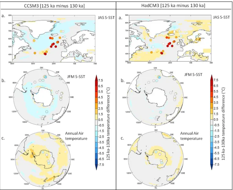
Fig. 5. Temperature anomalies estimated for four time-slices at 115 ka, 120 ka, 125 ka and 130 ka. a. Northern Hemisphere air temperature and SST anomalies. SST anomalies are calculated relative to modern summer SST taken at 10 m water-depth from the World Ocean Atlas 1998 (following the MARGO recommendations,Kucera et al., 2005, months used to estimate modern SST at site locations are July, August and September). b. 2suncertainties of temperature anomalies in the Northern Hemisphere taking into account the error on the temperature reconstruction and the propagated dating errors. c and d. Same as a. and b. for the Southern Hemisphere. Summer months used to estimate modern SST at site locations are January, February and March. The bigger the dot is, the larger the anomaly is. Warming (cooling) vs modern temperature is represented in orange (blue).

(11)

locations is of 0.44"_{C. Similar to the calculations of temperature}

anomalies in marine records (Section2.3), we show here simulated summer SST anomalies deﬁned as JAS for the Northern Hemisphere and JFM for the Southern Hemisphere. For polar ice cores, we consider annual temperature anomalies at the locations of the Antarctic ice cores and the precipitation-weighted temperature anomaly at the location of the NEEM Greenlandic ice core (Figs. 6e7).

3. Results 3.1. LIG timeseries

The evolution of synchronised surface air and sea surface tem-perature records over the LIG (Fig. 4) highlights several major features. We highlight an asynchronous establishment of peak interglacial temperatures between the two hemispheres across the LIG by calculating the average date at which the maximum LIG temperature peaks occurs for the Southern Hemisphere records on one side (Fig. 4; records [27]e[47]; note that when a maximum value was not clearly identified in the record, we took the date where a clear change of slope is marked) and for the North Atlantic high latitude region records on the other side (Fig. 4; records [10] and [14]e[26], excluding the record from site CH69-K09 [24] for which it is difficult to unambiguously identify a temperature maximum). For the Southern hemisphere records, we obtain a date of 129.3 ka associated with a standard deviation of 0.9 ka while we obtain a younger date of 126.4 ka associated with a standard de-viation of 1.9 ka for the North Atlantic high latitude records. This result hence illustrates the hemispheric differences highlighted in our database. Air temperature maximum conditions at the NEEM site [1] in Greenland occur at 126.9 ka, synchronously within dating uncertainties with the warmest conditions in the North Atlantic high latitudes. Although concerns about the synchronisation pre-cluded our use of European vegetation data here, we note that the time of maximum temperature (in both the warmest and coldest month) across Europe was also deduced to be around 127 ka (Brewer et al., 2008). In the Nordic Seas, SST records (records [2]e [7]) are characterised by small amplitude temperature changes across the LIG, in particular because of the limitation of N. pachydermasinistral percentages to record STT variations at low temperatures (see Section 2.2). Because the temperature uncer-tainty associated with each record after being aligned onto AICC2012 is about 3e4 "_{C, it is difficult to determine with}

confidence the timing of maximum surface temperature peaks in this region. No significant maximum temperature peak is identified in records [2], [3], and [4] located at the highest latitudes (between 68"_{N and 70}"_N; _{Fig. 4}_{). Still, the establishment of interglacial}

temperature seems to occur at 122.5 ka, and 122.7 ka in MD95-2009 [7] and MD95-2010 [5] respectively. In the Labrador Sea, re-cords [11] and [12] do not record unambiguously a temperature maximum while a LIG temperature peak is identiﬁed at 124.4 ka in record [21].

Our data synthesis also reveals large regional climatic vari-ability, in particular in the North Atlantic high latitude region. For example, the summer SST record from core MD95-2014 exhibits a deglacial temperature increase toward a maximum, directly fol-lowed by a smooth temperature decrease (Fig. 4, [10]). At other sites, such as the coring sites of ENAM33 and ODP980, maximum summer SSTs prevail for 7e13 ka before cooling and glacial inception take place (Fig. 4, [8] and [14]). Also M23414-9 and SU90-39 SST records clearly exhibit a two-step deglaciation interrupted at 130 ka (Fig. 4, [16] and [18]). Such a pattern has also been recently shown and discussed in a new SST record from the Alboran Sea located at 36"_12.30_{N (core ODP976;} _{Martrat et al.,}

2014) while this is not a feature that is unambiguously observed in the other records included in our synthesis (located above 40"_{N). However, the likelihood of recording such a}

millennial-scale feature is highly dependent on the temporal resolution of the records. Regional variability is observed in the Southern Hemisphere with a clear temperature overshoot in Antarctic sur-face air temperature records (records [44]e[47]) and possibly in DSDP-594 [34]. This overshoot is not visible in other Southern Ocean marine records.

Finally, our synthesis suggests a larger magnitude of tem-perature changes over Antarctica (3.5"_{C temperature change on}

average in ice core records between 130 and 115 ka) than at the surface of the surrounding Southern Ocean. Contrasts are also observed within the Southern Ocean with marine records at the highest latitudes (up to 50"_{S) showing a smaller amplitude of}

temperature change between 130 and 115 ka (1.2"_{C on average)}

than for marine records north of 50"_{S (2.5} "_{C on average).}

Similarly, Nordic Seas records north of 67"_{N only exhibit less}

than a 2"_{C amplitude in the temperature change while}

MD95-2009 [7] records up to a 10"_{C temperature change over}

Termi-nation II. However, because SST variations below 6.5"_{C are not}

well captured by the percentages of the polar species N. pachyderma sinistral (Govin et al., 2012), the amplitude of temperature changes may be underestimated in the Nordic Seas. Still, overall the strongest amplitudes of temperature changes are recorded in the Northern Hemisphere high latitudes compared to the Southern Hemisphere high latitudes (e.g. SU90-39 [18] and SU90-08 [22]).

3.2. LIG data-based time slices

Our four data-based time slices capture the major features characterising the spatial sequence of events described in Section

3.1(Fig. 5). In particular, the 130 ka time slice clearly illustrates the asynchrony previously reported between the Northern and the Southern Hemisphere high latitudes (e.g.Masson-Delmotte et al., 2010; Govin et al., 2012). It also reveals SST signiﬁcantly cooler-than-present-day sea surface conditions (e.g. up to 7.5 ± 3 "_C

cooler for [20]) in the high latitudes of the Northern Hemisphere while temperatures were slightly warmer than today (1.7 ± 2.5"_C

on average) in most of the Southern Hemisphere sites.

Warmer than present day climatic conditions are visible on the 130, 125 and 120 ka time slices in the Southern Hemisphere, while

Table 1

Forcing and boundary conditions used in CCSM3 and HadCM3 simulations ( Otto-Bliesner et al., 2013; Lunt et al., 2013for more details). Greenhouse gas concentra-tions used for the HadCM3 simulaconcentra-tions are those speciﬁed by PMIP3. They were deduced from records measured on the EDC ice core displayed on the EDC3 time-scale (Spahni et al., 2005; Loulergue et al., 2008; Lüthi et al., 2008). Similar values are obtained when using the AICC2012 time scale. Greenhouse gas concentrations used for the CCSM3 simulations are higher than the ones taken in the PMIP3 LIG pro-tocols. They were deduced from the EDC greenhouse gas concentration records displayed on the EDC3 timescale but represent the peak overshoot values occurring at 128e129 ka.

CCSM3 HadCM3

130 ka 125 ka PI 130 ka 125 ka PI Geography Modern Modern Modern Modern Modern Modern Ice Sheets Modern Modern Modern Modern Modern Modern Vegetation Modern Modern Modern Modern Modern Modern CO2(ppmv) 300 273 289 257 276 280 CH4(ppbv) 720 642 901 512 640 760 N2O (ppbv) 311 311 281 239 266 270 Solar constant (W m$2₎ 1367 1367 1365 1365 1365 1365 Orbital 130 ka 125 ka 1990 130 ka 125 ka 1950

(12)

they are only unambiguously observed on the 125 and 120 ka data-based time slices in the Northern Hemisphere.

3.3. Model-data comparison at 130 ka and 125 ka

Figs. 6 and 7display the model-data comparison for the 130 ka time-slice and the 125 ka time slice respectively. Absolute dating should be considered when comparing our new LIG synthesis to model outputs. Because the data-based time slices represent 2 ka time windows that have been calculated every 5 ka from 130 to 115 ka, dating errors affecting the palaeoclimatic records un-certainties (including the absolute dating error of the AICC2012 time scale, i.e. less than 1.6 ka during the LIG,Bazin et al., 2013) should have a limited impact on the main patterns highlighted in the model-data comparison.

In the Northern Hemisphere high latitudes, both the HadCM3 and CCSM3 simulations exhibit at 130 ka signiﬁcantly warmer summer sea surface conditions compared to present-day. In contrast, reconstructed summer temperatures display cooler

conditions compared to present day. Note also that the CCSM3 130 ka simulation is warmer than the HadCM3 130 ka simulation. This is predominantly due to the difference in GHG concentration values used where CCSM3 has a CO2value ~50 ppmv higher than

HadCM3, though also inﬂuenced by the different sea ice sensitiv-ities of the two models (Table 1).

In the Southern Ocean, the discrepancy between simulated and reconstructed summer SST is smaller than in the Northern Hemi-sphere high latitudes. Still, LIG modelled summer SST are similar to present-day ones in both model simulations while the data from the Southern Ocean illustrate surface oceanic conditions warmer by to up to 3.9 ± 2.8"_{C compared to present day (i.e. [29]). Modelled}

annual air temperatures above Antarctica are similar to present-day at 130 ka in both CCSM3 and HadCM3 simulations. However, all reconstructions from Antarctic ice cores suggest temperatures 1.5 ± 1.5"_{Ce2.5 ± 1.5}"_{C warmer than for present-day. Thus, our}

model-data comparison at 130 ka illustrates that these two models correctly simulate neither the cooler-than-present-day conditions in the northern high latitudes nor the warmer-than-present-day

Fig. 6. 130 ka Model-data comparison for the time slice at 130 ka, using the (left panel) CCSM3 and (right panel) HadCM3 models. a. Summer SST temperature anomalies from the marine sediment data (dots) superimposed onto model JulyeAugusteSeptember SST simulation in the Northern Hemisphere; b. Summer SST temperature anomalies from the marine sediment data (dots) superimposed onto the model JanuaryeFebruaryeMarch SST simulation in the Southern Ocean; c. Annual surface air temperature anomalies from the ice core data (dots) superimposed onto the model annual simulation.

(13)

conditions in the southern high latitudes. In other words, the linear response to summer insolation changes in the Northern Hemi-sphere and the lack of response to orbital forcing in the Southern Hemisphere are not consistent with air and sea surface tempera-ture reconstructions.

In the Northern Hemisphere high latitudes, the CCSM3 125 ka simulation exhibits higher computed than reconstructed SST by up to 6"_{C in speciﬁc locations (e.g. [16], [17] and [18]). It is in}

agree-ment within less than 2"_{C with the reconstructed data records at}

some other locations (e.g. [22], [23], [25] and [26]). Considering the uncertainty range associated with SST estimates, HadCM3 results are generally in good agreement with Northern Hemisphere high

latitudes SST data for 125 ka. However, both models fail at repro-ducing the reconstructed temperature anomalies at the sites characterised by cooler than present day sea surface conditions ([5], [6], [7], [21] and [24]). Note that the differences observed between the CCSM3 and HadCM3 simulations are likely related to their sea ice sensitivities with CCSM3 being more sensitive in the Northern Hemisphere and less sensitive in the Southern Hemisphere than HadCM3 (Otto-Bliesner et al., 2013).

Although they simulate warmer conditions over the Greenland ice sheet, neither of the 125 ka simulations are able to produce a warming as strong as that estimated from the NEEM ice core (7 ± 4 "_{C at 125 ka) in precipitation-weighted air}

Fig. 7. 125 ka Model-data comparison for the time slice at 125 ka, using the (left panel) CCSM3 and (right panel) HadCM3 models. a. Summer SST temperature anomalies from the marine sediment data (dots) superimposed onto model JulyeAugusteSeptember SST simulation in the Northern Hemisphere; b. Precipitation-weighed temperature anomaly reconstructed from the NEEM ice core (dot) superimposed onto precipitation-weighed temperature simulated above Greenland; c. Summer SST temperature anomalies from the marine sediment data (dots) superimposed onto the model JanuaryeFebruaryeMarch SST simulation in the Southern Ocean; d. Annual surface air temperature anomalies from the ice core data (dots) superimposed onto the model annual simulation.

(14)

temperature (Fig. 7b). However, an uncertainty of ±4 "_{C is}

associated with the NEEM precipitation-weighted temperature anomaly. Furthermore, interpretation of Greenland water iso-topic proﬁles in terms of temperature remains challenging due to the seasonality affecting the precipitations, changes in ice sheet topography (e.g.Vinther et al., 2009; NEEM c. m. 2013), and the possible effects of boundary conditions such as sea ice extent on the relationship between temperature and isotopic content (Sime et al., 2009).

In the Southern Ocean, data and simulations present fairly similar summer sea surface conditions at 125 ka compared to 130 ka given the associated temperature uncertainty. As for Ant-arctic surface air temperature, cooler than present day annual conditions are observed in the 125 ka CCSM3 simulation. The HadCM3 125 ka simulation shows warmer-than-present annual conditions in agreement within 2"_{C with the climatic conditions}

depicted in ice core data. Note that for both models, simulations represent best the warmer-than-present-day conditions at the location of ice core data when considering winter air temperature

over Antarctica (simulation data not shown). This seasonal aspect would deserve further investigations.

Fig. 8represents the difference between the 125 ka and the 130 ka climatic conditions. It strengthens our observations about the climatic changes in the course of Termination II in the Northern Hemisphere. Indeed, it provides a model-data comparison free from the uncertainty associated with the choice of the reference tem-perature in both the models and the data for present day conditions (Section2.4). This comparison highlights that the magnitude of Northern Hemisphere SST changes between 130 and 125 ka is not represented in both models simulations. The warming observed in the data is underestimated by up to 5"_{C in the HadCM3 simulation}

while a slight cooling is produced in the CCSM3 simulation. Both models correctly simulate the absence of signiﬁcant cli-matic changes in the Southern Ocean between 130 and 125 ka. Finally, ice core data depict a stable or slightly colder climate (be-tween 0 ± 1.5"_{C and $1.5 ± 1.5}"_{C) that is reproduced in the CCSM3}

[125 ka minus 130 ka] simulation while HadCM3 produces a slight warming (between 0.5 and 1.5"_C).

Fig. 8. Temperature difference between 125 ka climatic conditions and 130 ka climatic conditions both as recorded in Antarctic ice core and marine sediment data and as simulated by CCSM3 (left panel) and HadCM3 (right panel). In both models, simulated Summer SST are calculated as a temperature average over the months JFM and JAS for the a. Northern Hemisphere and b. the Southern Hemisphere Summer SST respectively. c. Simulated annual air temperatures are compared with air temperature anomalies inferred from Antarctic ice cores.

(15)

4. Discussion

4.1. Potential and limits of the new LIG spatio-temporal data synthesis

The SST records of our data synthesis have been derived from various methods. The MARGO SST synthesis for the Last Glacial Maximum time period shows that using different microfossil proxies yield discrepancies in SST estimates above 35"_{N (}_MARGO

project members, 2009). Unfortunately, quantitatively assessing the temperature uncertainties related to the use of SST records based on different methods in our case is difficult since only two cores MD03-2664 and SU90-08 benefit from multiple SST re-constructions. For site SU90-08, the comparison of the MAT-based SST reconstruction ([23],Fig. 4) with the alkenone-based SST reconstruction [22] shows that major transitions are recor-ded at the same time but higher maximum LIG temperature and larger amplitude changes are observed in the MAT-based sum-mer SST reconstruction compared to the alkenone-based SST reconstruction. However, alkenone-based SST is usually inter-preted as reflecting annual conditions (Müller et al., 1998; Sachs et al., 2000), while MAT-based SST reflects summer conditions. SST reconstructions based both on the Mg/Ca ratio [13] and MAT [12] are available for core MD03-2664. Mg/Ca ratio-based tem-peratures are systematically lower than MAT-based summer SST but higher than MAT-based winter SST.Irvali et al. (2012)suggest that this pattern illustrates that the Mg/Ca ratio-based SST esti-mates might reflect spring conditions. As a result, SST signals from those two cores highlight the difficulty of comparing SST records from different proxies, because reconstructed SSTs may represent different seasonal or annual signals. Previous studies have already reported this issue and also highlight an additional bias derived from the different calibration datasets used in the SST reconstructions (e.g.de Vernal et al., 2006; Hessler et al., 2014). Overall, combining LIG SST reconstructions inferred from different methods may induce inconsistencies in the recon-structed SST records, creating difficulties when comparing ab-solute values. However, this issue is reduced in our case since SST estimates derived from faunal assemblages dominate (30 out of 42 records). Additional high-resolution SST records based on various proxy methods would be required to carefully assess quantitatively how much the use of various SST reconstruction methods influences the temporal LIG characteristics highlighted in this study.

Mean annual or summer SST for each marine core location were extracted at 10 m depth from the 1998 World Ocean Atlas (WOA98) to develop a comparison to modern time annual and summer SST. Core top SST reconstructions can diverge from the WOA98 SST (Table A1) and this may introduce systematic offsets in temperature anomaly calculations. Using only core top SST estimates based on the same proxy as LIG SST reconstructions is not possible because this top-core information is available in a few selected records only (Fig. A1). Using core top SST values as modern time references is also complicated by the perturbation or the loss of most recent sediments during coring procedure. When available, we compare the temperature anomaly obtained from core top SST and modern WOA SST as reference temperatures. Fig. A1presents the data-based time slices with temperature anomalies calculated with the core-top SSTs as references. It illustrates that the major climatic features and patterns described on Fig. 5 are also visible when considering core top SST as present-day reference, i.e. an early Southern Hemisphere high-latitude warming compared to the Northern Hemisphere high-latitudes, longer warmer-than present conditions in the Southern Hemisphere and larger amplitude of temperature changes in the high Northern latitudes.

In addition, we are aware that considering summer (JAS SST in the Northern Hemisphere; JFM SST in the Southern Hemisphere) temperature at 10 m water-depth as modern reference might be a poor representation of the modern habitat of foraminiferal species in terms of season and water-depth (e.g.Tolderlund and B!e, 1971; Kohfeld et al., 1996; Simstich et al., 2003; Jonkers et al., 2010). However, we consider that it represents the most appropriate choice here to calculate past temperature anomalies, because it corresponds to the calibration depth and season that are included in the calibration core top database (e.g.Kucera et al., 2005; MARGO c. m. 2009) used in SST transfer functions to reconstruct past SST changes. Also, we highlight in the previous paragraph that we observe similar major climatic features and patterns when comparing temperature anomalies calculated vs WOA or core top values, which suggests that the choice of WOA modern values at 10 m water-depth has little effect on the main results of our study. Estimated uncertainties are about 2.6"_{C on average for marine}

sediment cores and set at 1.5"_{C for Antarctic ice cores and 4}"_{C for}

the NEEM ice core. This means that they are frequently of the same amplitude as the calculated temperature anomaly itself. However, it is possible to highlight with conﬁdence some climatic patterns in the Southern Hemisphere and the North Atlantic region based on observations made on multiple records. For instance, we consider that a warmer than present-day Southern Ocean by about þ2"_{C is a}

robust climatic feature on the 125 and 130 ka data-based time slices since it is observed in most of the considered marine records even though taken individually each SST anomaly is associated with an error of similar magnitude.

Although we are confident in the age models developed for the Southern Ocean and North Atlantic marine records, one should keep in mind that defining robust and coherent chronologies for SST records from the Nordic Seas remains difficult and that the associated relative uncertainty is large (~3e4 ka). This feature re-sults from the current limitations associated with SST reconstruc-tion method based on the percentage of the polar species N. pachydermasinistral, and the difficulty to identify unambigu-ously stratigraphic markers between cores. Consequently, it is difficult to identify robust climatic patterns in this region. Future high-resolution SST records based on alternative proxies and the identification of new stratigraphic markers (e.g. tephra horizons,

Davies et al., 2014) should help to improve chronologies for palaeoclimatic records from in this region.

While previous compilations already demonstrated warmer-than-present-day conditions prevailing during the LIG, the emphasis of these compilations was on quantifying the maximum in temperature warmth rather than on the temporal evolution of the climatic conditions across the time-period. The data synthesis ofTurney and Jones (2010)reported the early Antarctic warming but their work was lacking a common temporal framework be-tween climatic records. Our work is the ﬁrst LIG compilation associated with a common time frame between marine and ice high-latitude records from both hemispheres. This enables to provide a detailed spatio-temporal information on the evolution of high-latitude temperature throughout the LIG. We also propagate age uncertainties and include SST reconstruction method errors in order to map for the ﬁrst time high latitude temperature anomalies for four time slices covering the LIG.

4.2. GCM snapshot simulations vs data-based time slices: mismatch and implications

Otto-Bliesner et al. (2013) used the LIG compilations from

Turney and Jones (2010)andMcKay et al. (2011)to benchmark two CCSM3 snapshot simulations performed under 125 and 130 ka conditions for the orbital and greenhouse gas concentration