HAL Id: hal-01761324
https://hal.archives-ouvertes.fr/hal-01761324
Submitted on 8 Apr 2018
HAL is a multi-disciplinary open access
archive for the deposit and dissemination of sci-entific research documents, whether they are pub-lished or not. The documents may come from teaching and research institutions in France or abroad, or from public or private research centers.
L’archive ouverte pluridisciplinaire HAL, est destinée au dépôt et à la diffusion de documents scientifiques de niveau recherche, publiés ou non, émanant des établissements d’enseignement et de recherche français ou étrangers, des laboratoires publics ou privés.
A quantitative, space-resolved method for optical
anisotropy estimation in bulk carbons
Adrien Gillard, Guillaume Couégnat, Olivier Caty, Alexandre Allemand,
Patrick Weisbecker, Gérard Vignoles
To cite this version:
Adrien Gillard, Guillaume Couégnat, Olivier Caty, Alexandre Allemand, Patrick Weisbecker, et al.. A quantitative, space-resolved method for optical anisotropy estimation in bulk carbons. Carbon, Elsevier, 2015, 91, pp.423-435. �10.1016/j.carbon.2015.05.005�. �hal-01761324�
A quantitative, space-resolved method for optical
anisotropy estimation in bulk carbons
Adrien P. Gillarda, Guillaume Cou´egnata, Olivier Catya, Alexandre Allemanda,b,
Patrick Weisbeckera, Gerard L. Vignolesa,⇤
aUniversity of Bordeaux,
Laboratoire des Composites ThermoStructuraux (LCTS) UMR 5801: CNRS-Herakles(Safran)-CEA-UBx
3, All´ee de La Bo´etie, 33600 Pessac, France Tel: (+33) 5 5684 3305
bCEA DAM - Le Ripault, BP 16, 37260 Monts, France
Abstract
This paper presents an innovative and quantitative method for characterization of bulk carbons using polarized light microscopy. It yields maps of transverse preferential orientation and quantitative transverse anisotropy. It can be utilized on any region observable with an optical microscope, at any attainable scale. It requires a set of micrographs from the same region of a carbon-based sample at di↵erent combinations of polarizer and analyzer positions. Applications of the technique to several actual carbon-based materials are presented and discussed. Keywords: Polarized light optical microscopy; anisotropy; bulk carbons
⇤Corresponding author
Email addresses: gillard@lcts.u-bordeaux1.fr (Adrien P. Gillard),
couegnat@lcts.u-bordeaux1.fr(Guillaume Cou´egnat), caty@lcts.u-bordeaux1.fr (Olivier Caty), allemand@lcts.u-bordeaux1.fr (Alexandre Allemand),
weisbecker@lcts.u-bordeaux1.fr(Patrick Weisbecker), vinhola@lcts.u-bordeaux1.fr(Gerard L. Vignoles)
*Manuscript
1. Introduction
Bulk carbons di↵er from ideal graphite by a variable amount of structural and textural defects; they can therefore be identified and classified through a measure of their anisotropy. Various techniques provide that information, such as polarized light optical microscopy (PLOM), Raman microspectroscopy, X-ray di↵raction or transmission electron microscopy (TEM). Even if these techniques bring good qualitative information on the anisotropy, having a quantitative measure is often averaged over a selected area. In particular, PLOM is used to measure the extinc-tion angle Aebetween crossed polars, and the values are always given as averages
over the whole imaged region. Moreover, this technique depends up to now on the existence of some specific geometrical arrangement of the carbon phases (circular or planar). Extending this traditional method to any kind of bulk carbon sample, without any prior knowledge of the orientation layout, is a rewarding challenge. Due to their intrinsic structural anisotropy, carbon-based materials are uniaxially birefringent, which implies that the intensity and phase of light reflected on them depend on the polarization of the incident light. In 1965, Taft and Philipp [1] and later Ergun et al. [2] discussed the birefringence of graphite. They had measured the reflectance and the dielectric constant in the a-direction of the crystal. Then, Greenaway and Harbeke [3] introduced the reflectivity at non-normal incidence. They used the Drude model and characterized the reflectivity in both the a and c directions in graphite. In 1973, Johnson and Dresselhaus [4] brought a mea-suring technique of the dielectric constants in both directions, in the visible band. From this point on, the optical properties of graphite may be considered as well known. Bulk carbons (i. e. polymer-derived or pitch-derived carbons, including fibers, or gas-deposited pyrolytic carbons) have a complex structure locally simi-lar to that of graphite, but containing many kinds of structural and textural flaws.
Hence, a bulk carbon can be considered as a more or less isotropic graphite, and the knowledge of graphite properties can be used to model the optical behavior of bulk carbons.
In 1971, Diefendorf and Tokarsky [5, 6] introduced the use of a measurement, commonly carried out in petrography [7]: the determination of the extinction an-gle of carbons, using polarized light microscopy, as a quantitative way to measure their anisotropy. It is a probe of the defects of the crystal lattice, over a selected area and at a specific wavelength. An amorphous bulk carbon would have a low extinction angle whereas a graphite would have a high extinction angle, up to 25°at 550 nm [8]. All bulk carbons can be found in between. They applied it suc-cessfully to several carbon fibers [5]. This method provides a semi-quantitative measurement of the anisotropy over a selected region [9]. Indeed, its usual im-plementation is slightly operator-dependent. The extinction angle was also used for qualitative analysis of the anisotropy in ex-pitch carbon matrices [10, 11]. In 2000, Bourrat et al. [12] published a classification of low temperature pyrolytic carbons (or pyrocarbons), based on the azimuth opening (OA) of a di↵raction fringe under electronic microscopy. The link with observation under polarized light is analyzed, showing the importance of the extinction angle to characterize carbons. This was later confirmed by Reznik and H¨uttinger [13], with a some-what distinct terminology for pyrocarbon classification [14]. In 2004, Pfrang and Schimmel [15] presented a quantitative method for measuring the extinction an-gle without operator-related uncertainties; they showed that biases can exist with respect to more manual measurements. However, they only could work on flat deposits, and their method only provided an average value over the whole imaged domain. Similarly, in 2012, Li Miaoling and his team [16] presented a method based on the polarized light sensitivity of pyrocarbons. They obtained a qualita-tive map of optical anisotropy from polarized light microscopy imaging. Again,
their method depended on the knowledge of the local orientation, using a silicon wafer to ensure a planar pyrolytic carbon deposition. They used the di↵erences of anisotropy in the material for segmentation purposes. On the other hand, in 2006, Vallerot and Bourrat [8] studied in more detail the optical properties of a series of pyrocarbons. They identified them using the extinction angle, studying its dependence on the wavelength. Using a spectrophotometer, they produced a large amount of data on reflectivities, but their data was, as usual, not resolved in space. Bortchagovsky [17, 18] has proposed a deeper treatment of the theoretical aspects of ellipsometry applied to pyrolytic carbons, and derived a more rigorous expression of the extinction angle as a function of the intrinsic properties of the materials.
Having a space-resolved method for anisotropy measurement rests on the pos-sibility of determining with the same resolution the local orientation of the carbon phases. The orientation can be defined as the direction of polarization where the material has the highest reflectance. This orentation map may be obtained quanti-tatively by the sensitive-tint method. In this technique a transparent, birefringent crystal is placed in between the crossed polarizer and analyzer. The thickness of the crystal is such that the phase change between the two principal axes is one wavelength in the middle of the visible spectrum ( ). Thus, if this crystal is in-serted at 45° with respect to the vibration direction of the polarized light the only wave length extinguished will be , all other wavelengths will be transmitted due to their ellipticity. Hence, the orientation of the layer planes in graphite can be determined by their color, i. e. depending whether they are aligned parallel or perpendicular to the plane of polarization, they show up distinctly as either red or blue. This technique has been used for the qualitative determination of the texture of carbon fibers [19] and of carbonaceous mesophase in bituminous coals
[20]. Quantitative use has been made for e. g. grains in a Beryllium polycrys-tal [21] and Poly(trimethylene terephthalate) (PTT) spherulites [22], making use of correlations between the color shift and the orientation. . Polarized Raman spectroscopy has also been used recently for the same purpose [23]. However, it is possible to do the same thing with simpler tools, namely, PLOM with polar-izer and an analyzer. For instance, in 2003, F. Massoumian et al. [24] developed a method to measure the local optical orientation, and applied it to supra-conducting YBaCuO crystals. It was based on polarized light sensitivity under microscopy imaging, and yielded orientation maps of the material phases. This method is eas-ily adaptable to bulk carbons, but this has never been carried out, to the authors’ knowledge.
Extending these preceding works, we have developed a new method for estimat-ing the anisotropy regardless of the orientation in the material. It provides maps of local orientation and of quantitative anisotropy of any region observable with an optical microscope, for characterization purposes. In a first part, the theoretical aspects of the problem will be considered. The second part presents briefly the studied carbon-based materials samples and methods, and the third part discusses the obtained results.
2. Principle
2.1. Optical behavior of bulk carbons under polarized light at normal incidence In this section, we will derive rigorous expressions for the quantities of inter-est, following the ideas of Bortchagovsy [18]. Let us assume the carbon-based materials are composed of tiny coherent regions called grains, 1 to 100 nm wide. Each grain has its own 3D orientation, fully described by two angles: the hori-zontal orientation ✓g and the vertical tilt angle ✓t, as sketched in Figure 1, and a
3D anisotropy ⌧3D. Viewed in 2D, a tilted grain presents an apparent anisotropy,
equal to the actual 3D anisotropy only if the tilt angle is zero. On the other hand, the more the grain is parallel to the surface, the more it looks isotropic.
Top view Side view
3D view
Figure 1: Orientation in a selected region of a birefringent material
Figure 2 depicts the placement of the required elements for optical microscopy under polarized light. In what follows, the light at any part of the system is repre-sented by a monochromatic electric fieldEx and its intensity Ix, propagating into
the vacuum at a 550 nm wavelength (2.25 eV). The light emitted by the source E0 is not polarized and its intensity is I0. After going through the polarizer, it
becomes the incident light represented by an electric field Ei and an intensity Ii.
It is then reflected on the carbon sample surface (Er,Ir). Then, after crossing the
analyzer, it becomes (Ea,Ia).
Any uni-axial birefringent material has two main reflection directions: ordi-nary and extraordiordi-nary, with associated complex reflection coefficients roand re,
respectively. We will define an orthogonal reference setnO,ex,ey
o
illumi-CCD CAMERA LIGHT SOURCE (2.25eV) ANALYZER POLARIZER CARBON MATERIAL
Figure 2: Schematics of the microscope to produce micrographs under polarized light.
nated surface, the angle between ex and the ordinary direction being denoted ✓g.
Note that ✓gbeing an orientation, it is defined modulo ⇡. Then, each pixel of the
image corresponds to a tiny region of the material with an angle ✓g(x, y) and two
reflectivities ro(x, y) and re(x, y).
2.2. Expression of the reflected intensities
We will first consider the case where the grain has no tilt. The polarizer will be represented by the directionep and the analyzer by ea. The ordinary and
sketched in figure 1. 8 >>>>> >>>>> >< >>>>> >>>>> >: ep = excos ✓p+eysin ✓p ea = excos ✓a+eysin ✓a eo = excos ✓g+eysin ✓g ee = exsin ✓g+eycos ✓g (1)
The expression of the incident light is given by taking the scalar product of the initial non-polarized lightE0and ofep:
8 >>>>> < >>>>> : Ei = ep r I0 2 Ii = I20 (2) The reflected light is obtained by taking the scalar product of the incident lightEi
and of the material orientation vectoreo. Expressed in the local material reference
frame {O, eo,ee}, we have :
8 >>>>> < >>>>> : Er = r I0 2 h rocos ✓gpeo+resin ✓gpee i Ir = I20 h |ro|2cos2✓gp+|re|2sin2✓gp i (3)
where ✓gp = ✓g ✓p. To simplify the expression of the intensity Ir, we introduce
the reflection coefficient R and the optical anisotropy ⌧ as: 8 >>>>> < >>>>> : R = |ro|2+|re|2 ⌧ = |ro| 2 |r e|2 |ro|2+|re|2 (4) so that Eq. 3 becomes :
Ir = I04R
h
1 + ⌧ cos 2✓gp
i
(5) From Eq. 5 it is seen that the intensity after a reflection on a bulk carbon can be decomposed into a steady component and a sine component.
2.3. Expression of the analyzed intensity without tilt
The expression of the light after the analyzer is obtained with the scalar prod-uct of the reflected electric fieldEr and of the analyzer directionea:
8 >>>>> >>>>> >>< >>>>> >>>>> >>: Ea = pI 0 2 h
r0cos ✓gpcos ✓ga+resin ✓gpsin ✓ga
i ea Ia = I04R h⇣ |ro|2+|re|2 ⌘ ·⇣1 + cos 2✓gpcos 2✓ga ⌘ +⇣|ro|2 |re|2 ⌘ ·⇣cos 2✓gp+cos 2✓ga ⌘ +(rore+rore) · sin 2✓gpsin 2✓ga i (6)
where ✓gp = ✓g ✓pand the overlined quantities denote complex conjugates.
This equation may be rewritten by the introduction of the previously defined parameters ⌧ and R. Moreover, introducing the phase shift of the ordinary reflec-tion o = arg (ro), and recalling that there is no phase shift in the extraordinary
direction [8], the expression of the intensity becomes: Ia= I04R h 1 + cos 2✓gpcos 2✓ga+ ⌧ ⇣ cos 2✓gp+cos 2✓ga ⌘ + p1 ⌧2cos osin 2✓gpsin 2✓ga
i (7)
We see that the analyzed light intensity contains four components. The first one is isotropic, the second one is only related to the polarizer and analyzer angles; the third one depends on the preceding quantities and on the anisotropy, and the fourth one depends in addition to the phase shift factor.
2.4. The extinction angle as a quantitative measure of the anisotropy
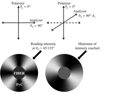
The classical method for measuring the extinction angle is illustrated by fig-ure 3. It is restricted to a fixed material orientation at ✓g = 45°, the polarizer
di-rection being ✓p =0°. It supposes the initial knowledge of the ordinary direction
✓g. In the particular case of pyrocarbons, the basal planes of the material are
usu-ally deposited around fibers or parallel to a substrate. Figure 3 describes the case of a pyrocarbon deposed around a fiber, i.e. a carbon/carbon micro-composite.
A region at ✓g = 45° from the vertical has been selected. The polarizer is held
vertically (✓p = 0°) and the analyzer is initially horizontal (✓a = 90°). Then, the
analyzer is moved toward the polarizer and the intensity is read at the selected location. When the minimum of intensity is reached, the angle of displacement of the analyzer is equal to the extinction angle.
Reading intensity at θG = 45/135° Minimum of intensity reached Polarizer Polarizer Analyzer Analyzer θp = 0° θp = 0° θA = 90° θA = 90°-Ae FIBER PyC
Figure 3: Measurement of the extinction angle on a carbon/carbon microcomposite.
The theoretical expression of the classical extinction angle is obtained by searching the intensity minimum with respect to the analyzer angle :
dIa d✓a ✓ ✓a =Ae, ✓p= ✓g+ ⇡4[⇡] ◆ =0 (8)
tan 2Ae = |ro| 2 |r e|2 rore+rore = ⌧ p 1 ⌧2 1 cos o (9)
Eqs. 6 to 9 have introduced a difficulty: a separate knowledge of the real and imaginary parts of the reflection coefficients, or equivalently of ⌧ and cos o, has
to be known. Fortunately enough, it is possible instead to take advantage of the previous work of Vallerot and Bourrat [8]. Using a spectrophotometer coupled to a polarized microscope, they measured the extinction angle, optical phase shift, and the ordinary and extraordinary reflectances of numerous bulk carbons, enough to establish a database and a classification. Figure 4 is a graph of cos o vs. ⌧
obtained from this data-set. It appears that 1 cos o never exceeds 0.015, i.
e., o never exceeds 12°. Therefore, up to 1.5% error, the factor cos o may be
considered equal to 1 in practice.
0.5 0.6 0.7 0.8 0.9 1.0 1.1 0% 10% 20% 30% 40% 50% 60% 70% 80% 90% 100% cos( Φ o) Anisotropy (τ,%) Vallerot 2006 cos(ϕo) = 1+0.0286τ-0.0995τ²
Dark and smooth laminar Pyrocarbons
So, up to this precision, Aeis only a function of ⌧:
Ae = 12arctan p ⌧
1 ⌧2
!
± 1% (10)
Figure 5 is a plot of the extinction angle Ae vs. the optical anisotropy ⌧, as
computed from ref. [8]. Two measurements on graphite have been added [2, 8]. The curves describing eqs. 9 and 10 fit extremely well this data-set, except the
measurement on graphite by [8]. In other words, measuring Ae is equivalent to
measuring ⌧. Here we remind the reader that the measured Ae in this reference were systematically lower by 1-2° than the “classically measured” (i.e by man-ual operation) corresponding angles. So, highly textured pyrocarbons are in the [14° 18°] range instead of [16° 21°] as usually reported (or even higher, see e.g. [25]). 0 5 10 15 20 25 30 35 40 45 0% 10% 20% 30% 40% 50% 60% 70% 80% 90% 100% Extincti on An gl e (Ae ,° ) Anisotropy (τ,%) Ergun 1973 Vallerot 2006 τ | Linear τ | cos(ϕo) = 1 τ | cos(ϕo) = 1+0.0286τ-0.0995τ²
Figure 5: Relationship between the extinction angle and the optical anisotropy for various carbons.
seen as depending only on the variables ✓p, ✓a and the parameters ✓g, ⌧, Ae and I0R: Ia = I04R h 1 + cos 2✓gpcos 2✓ga+ ⌧ ⇣ cos 2✓gp+cos 2✓ga ⌘ + ⌧
tan 2Ae sin 2✓gpsin 2✓ga
# (11)
For sake of convenience, this expression will be rewritten under the following form, where the isotropic part of the signal is separated :
Ia = I04R h 1 + cos 2✓ap+ ⌧ ⇣ cos 2✓gp+cos 2✓ga ⌘ + ⇠sin 2✓gpsin 2✓ga i (12)
where ✓ap = ✓a ✓pand where we have defined the auxiliary quantity ⇠ as:
⇠ = ⌧
tan 2Ae 1 = cos o·
p
1 ⌧2 1 0 (13)
In some sense, ⇠ is a measure of the maximal quantity of light that manages to pass through crossed polars (✓ap = ⇡2).
From eq. (12-13) it is recognized that the analyzed light intensity contains three terms: one linked to the isotropic part of the material, the second and third ones being sensitive to the material birefringence. The theory may be extended to the case of tilted grains. Actually, ⌧ depends on the local tilt angle of the material, but the form of the equations remains the same, and the tilt-induced bias may be removed, as shown in appendix A. The modified equations developed there are the starting point of the experimental procedure that is described in the following part.
3. Proposed method
The traditional method for the measurement of Aeis not straightforward to use
since one has to choose a region with a known orientation ✓gp = 45°. Here, in
practice, it is enough to use eq. A.4 with cos o ⇡ 1 (therefore ⇠ ⇡ p1 ⌧2 1)
and identify directly ⌧, ✓t and ✓g(as well as I0R) from the evolution of Iaagainst
✓pand ✓a, i.e. from a set of micrographs obtained with distinct combinations of
these angles.
Many combinations of images may be imagined to design an identification method. Here, we have chosen to set independently ✓p and ✓a to the values set
⌦ = n0; ⇡4;⇡2;3⇡4o. Sixteen images of the same regions are acquired. We thus have a large amount of data redundancy, in order to improve the robustness (i. e. resistance to noise) of the method.
Summing over all images yields the orientation-independent part of the signal:
A = 1 2 X ✓a,✓p2⌦2 Ia ⇣ ✓a, ✓p ⌘ =I0R h 1 + ⌧ sin2✓ t i (14) Additionnally, two partial sums are of special interest :
S1 = X ✓a2⌦ Ia ⇣ ✓p=0, ✓a ⌘ Ia ✓ ✓p= ⇡2, ✓a ◆ = I0R⌧ cos2✓tcos 2✓g (15) S2 = X ✓a2⌦ " Ia ✓ ✓p= ⇡4, ✓a ◆ Ia ✓p= 3⇡4 , ✓a !# = I0R⌧ cos2✓tsin 2✓g (16)
From these sums, one gets two quantities : (i) the modulus of the orientation-dependent part of the signal :
B = qS2
1+S22 =I0R⌧ cos2✓t (17)
and (ii) the orientation angle ✓gitself :
✓g=arctan SS2 1
!
(18) Considering now the sum of all images taken with crossed polarizer and ana-lyzer (Maltese crosses), we have the following orientation-independent quantity:
C = 4X ✓p2⌦ Ia ✓ ✓p, ✓p+ ⇡ 2[⇡] ◆ = I0R⇠ cos2✓t ⇡ I0R ⇣ 1 p1 ⌧2⌘cos2✓ t (19)
We note that A, B and C are three independent quantities, allowing in principle the recovery of ⌧, ✓t and I0R. They are given by :
⌧ =sin✓2 arctan✓C B ◆◆ (20) I0R = A + B1 + ⌧ (21) cos2✓ t = IB 0R⌧ (22)
This ends up the specification of the procedure for the identification of the quan-tities of interest.
4. Experimental 4.1. Experimental setup
The study was performed with an optical microscope Nikon ME500L work-ing in reflection mode. This microscope is equipped with a HD CCD camera with digital output. The CCD camera (Nikon Digital Camera DMX 1200) con-verts linearly the intensity into an 8-bit grayscale value. The microscope is also equipped with graduated polarizer and analyzer. No modification was brought to the as-purchased setup, because its polarizer can be rotated by 45° steps. Di↵er-ent magnifications were used : ⇥5, ⇥20, and ⇥100, so that the smallest pixel size was 22 nm. Several snapshots of the same region under di↵erent angles of the polarizer and of the analyzer have been taken, as described in more detail below. A digital image alignment procedure is performed in order to compensate any possible movement of the sample between successive snapshots.
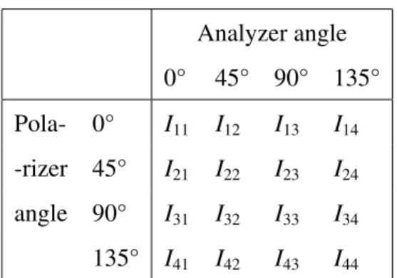
As specified in the preceding section, the same region is photographed at 4 an-gles of the polarizer (0°, 45°, 90° and 135°), and 4 anan-gles of the analyzer, totaling 16 micrographs for the same zone. Image alignment is carried out to eliminate any possible displacement between snapshots. Then, the procedure sketched above is used for the identification of the orientation ✓g, and of ⌧ and ✓t at each pixel.The
Analyzer angle 0° 45° 90° 135° Pola- 0° I11 I12 I13 I14 -rizer 45° I21 I22 I23 I24 angle 90° I31 I32 I33 I34 135° I41 I42 I43 I44
Table 1: Labeling of the sixteen images of a given region in the method.
intensity at a given pixel (having the same location on the 16 images after align-ment) is denoted by the symbols given in Table 4.1.
The computation is made as follows : • A is the half sum of all 16 images.
• S1=I11+I12+I13+I14 I31 I32 I33 I34.
• S2=I21+I22+I23+I24 I41 I42 I43 I44.
• B and ✓gare computed from eqs. 17-18.
• C = 4 (I13+I24+I31+I42).
• ⌧ and other quantities are obtained through eq. 22.
Extinction angles may be retrieved from ⌧, forming the anisotropy map. Fur-ther analyses can be performed on the maps: filtering, statistics, segmentation, etc. . .
4.2. Displaying the results
For each material observed, the natural light micrographs will be presented along with both an anisotropy map and an orientation map. An efficient way to
render the orientation is through a colored map, represented by a continuous ⇡-periodic color shift, while the anisotropy can be superimposed as a grayscale map by darkening the low anisotropy regions. Such a representation is consistent with the fact that when a material becomes isotropic, its orientation becomes undefined. Figure 6 presents a compact legend, used for all results.
Figure 6: Legend for the anisotropy and orientation maps. The disc-shaped legend on the right displays the orientation with a superimposed grayscale level indicating anisotropy.
The method is quantitative, so knowing the nature of the carbons (fiber and PyCs), an identification can be obtained through the anisotropy. A dark laminar
PyC would have ⌧ about 10% (Ae about 5°), a smooth laminar ⌧ about 30% (Ae
about 10°), a rough laminar ⌧ about 45% (Aeabout 15°).
4.3. Investigated materials
The selected materials were extracted from various carbon-fiber reinforced
Three types of samples were studied. First, we have studied a Cf/C composite
with a matrix obtained by several successive chemical vapor infiltration (CVI) runs, so that the pyrocarbon matrix is multi-layered. The fibers were XN05 ex-PAN carbon fibers (from Nippon Graphite Fiber Co.), with a rather low modulus, and arranged as a stitched stack of woven plies [26]. The sample surface has been mechanically polished. Second, we have investigated a bulk carbon sample ob-tained from pyrolyzed synthetic pitch [27], carbonized under high pressure. The sample has been mechanically polished too. The third sample has been extracted
from a 3D Cf/C composite, the preform of which is composed of M40 carbon
fibers (Toray Carbon Fiber Europe) (i.e. high-modulus fibers) arranged in straight bundles, and that has been densified using pyrolyzed pitch, carbonized under high pressure and then graphitized [28]. Here, an ion polishing procedure has been applied to the sample in order to preserve its surface state.
5. Results
The results obtained from this approach are presented in four parts. First, a study of similar fibers with various inclinations will be presented, in order to validate quantitatively the method. Then, the matrices of samples 1, 2 and 3 will be studied.
5.1. Validation of the method on inclined carbon fibers
The carbon fibers of composite 1 have been used for a quantitative validation of the method. They present distinct transverse and longitudinal anisotropy ratios, noted respectively ⌧? and ⌧k. The e↵ective anisotropy ⌧⇤ is in between, being a
function of the fibers inclination ✓f. This function can be written as the equation
of an ellipse in the (⌧; ✓t) coordinate space:
cos✓f ⌧? !2 + sin✓f ⌧k !2 = 1 ⌧⇤2 (23) Or: ⌧⇤ =✓⇣cos ✓f/⌧? ⌘2 +⇣sin ✓f/⌧k ⌘2◆ 1/2 (24) The inclination can be measured from the shape of the fiber elliptic sections, and more precisely the section circularity C = b
a:
✓f =arccos C = arccosba (25)
where a and b are respectively the major and minor axis lengths.
A comparison between both measures would show the efficiency of the estima-tion algorithm. Figure 7 presents a region composed of fibers and several layers of PyC matrix [26]. The anisotropy map shows the variation of the anisotropy between fibers with respect to the inclination. The inclined fibers present also a mean orientation.
Figure 7: A: Micrograph of a composite with a multi-layered pyrocarbon matrix (sample 1) . B: Qualitative sketch of the various components in the micrographs. C: Corresponding map of anisotropy. D: Corresponding map of orientation and anisotropy. Legend is presented on figure 6.
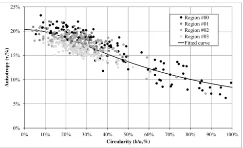
A campaign of measurements has been performed on many fibers from similar samples. Figure 8 is a plot of the anisotropy vs. circularity. The data points are rather dispersed, for several reasons. First, the scatter is due to the difficulty to fit the non-circular shape of the transverse section of the fibers, especially at low anisotropy (fibers close to 0°inclination). Other sources of data scatter may be the
polishing that creates local degradation of the surface, and the fact that some fibers are inhomogeneous. Nonetheless, it has been possible to fit the measurements with a reasonable agreement (std. dev. ⇡ 8%), yielding identified values of ⌧? =
8.4 ± 0.6% and ⌧k=20.3 ± 1.8%. The fitted curve also appears on the graph.
0% 5% 10% 15% 20% 25% 0% 10% 20% 30% 40% 50% 60% 70% 80% 90% 100% An isotr opy ( τ,% ) Circularity (b/a,%) Region #00 Region #01 Region #02 Region #03 Fitted curve
Figure 8: Quantitative analysis of fibers anisotropy. Plot of the raw data of anisotropy vs. circular-ity. Comparison with the theoretical relationship (eqs. 24-25).
5.2. Cf/C composite with multilayer pyrocarbon matrix
An application example of the quantification method is presented on a CVI-infiltrated Cf/C composite, featuring concentric layers of pyrocarbon (PyC) around
the carbon fibers. The sample was prepared by mechanical polishing. Considering the large amount of data obtained, we will focus here on selected regions, but the retained conclusions come from a more extended study.
We first discuss the di↵erent constituents presented on figure 9, i. e. in the center, a carbon fiber, and around it several PyC layers. Micrograph A shows the di↵erent layers – here, the grayscale contrast results essentially from the e↵ect of the surface roughness and the respective reflection coefficients of the constituents. The schematic B helps localizing the constituents and labels the di↵erent layers. The anisotropy map C is fully quantitative. The orientation map D confirms that the carbon matrices are deposited around the fiber. The di↵erence of anisotropy between the layers and, more interestingly, the columnar texture inside the layers are revealed.
The evolution of the anisotropy from the outer PyC layer up to the center of the fiber is plotted on figure 10. It confirms that (i) the fiber is less textured than the PyCs, and that (ii) the four successive layers are rough, dark, rough and rough laminar PyCs. From figure 9 it is seen that there are more anisotropic regions inside the layers, forming coherent domains the boundaries of which sometimes go through the layers. This is supported by the orientation map, showing single-orientation domains (regions with rather constant colors). It also shows the prop-agation of flaws and the boundaries between the coherent domains.
Figure 9: A:Micrograph of a small region in a composite with a multi-layered pyrocarbon matrix (sample 1). B: Sketch of the various components in the micrographs. C: Corresponding map of anisotropy. D: Corresponding map of orientation. Legend is presented on figure 6.
0% 10% 20% 30% 40% 50% 60% 0 5 10 15 20 25 30 35 An isotr opy τ ( %)
Position along radial axis (µm)
PyC 2 PyC 3
PyC 4 PyC 1
Fiber
5.3. Carbonized ex-pitch matrix
A carbonized material (sample 2, figure 11) has been studied with various magnifications. A representative sample has been extracted and mechanically pol-ished. Three regions have been micrographed at di↵erent scales: ⇥5 (A1), ⇥20 (B1) and ⇥100 (C1), and then analyzed (A2, B2 and C2 for the anisotropy maps, A3, B3 and C3 for the orientation maps respectively).
Figure 11: Micrographs of a carbonized ex-pitch carbon matrix at various scales (A1: ⇥5, B1: ⇥20, C1 : ⇥100). Corresponding maps of anisotropy (A2,B2,C2) and orientation (A3,B3,C3). Legend is presented on figure 6.
Figure 12 displays anisotropy histograms for the three selected scales. A com-mon feature of the three curves is the presence of two peaks, one at a low value,
associated to the pores and to possible secondary reflections, and the other one to the matrix, observed at 40-50% anisotropy (Ae ⇡ 15°) , i.e. similar to rough
lam-inar pyrocarbon , even though their formation mechanisms strongly di↵er. The
dark spots inside the most coherent regions are very likely due to the mechanical polishing, which probably have reduced the e↵ective anisotropy measured.
0% 10% 20% 30% 40% 50% 60% 70% 80% 90% 100% Anisotropy (τ,%) x5 x20 x100 Secondary reflections (resin or porosity)
Ex-pitch matrix reflection
Figure 12: Histogram of anisotropy from the region observed on figure 11.
A polar plot of the average anisotropy ratio as a function of the orientation is shown on figure 13. The main anisotropic directions can now be identified from such a plot. Interestingly, even at ⇥5 resolution, there is still some non-homogeneity of the orientation distribution resulting from the flow pattern around the large bubble, visible in figure 11-A1.
x5 x20 x100 Anisotropy (τ,%) 30% 20% 10% 00%
5.4. Highly graphitized Cf/C composite
The material that best illustrates the spatial resolution of the method is a sam-ple extracted from a Cf/C composite (figure 14). The natural light micrograph
(A) shows the pores in dark, the fibers (with bean-shaped sections) in intermedi-ate gray, and the matrix in light gray (around the fibers). The anisotropy map (C) and orientation map (D) provide useful information. First, the fibers appear more isotropic than the matrix (⌧ ⇡ 7%, Ae ⇡ 3°), but contain an oriented and textured
core (⌧ ⇡ 12%, Ae ⇡ 4°). The orientation is in the direction of the elongation of
the fibers section.
Second, the matrix appears very anisotropic (⌧ ⇡ 50%, Ae ⇡ 15°). It is
com-posed of coherent domains, with a single orientation inside them, preferentially oriented parallel to the closest fiber edge. These coherent domains are surrounded by thin dark lines which represent a boundary with a sharp change in the matrix orientation, is clearly visible on the orientation map. Smoothorientation changes are results of the flow pattern (e. g. after surrounding an obstacle) [29] but they
may become sharp after graphitization (transforming curves into broken lines).
This is in contrast with the pyrolyzed pitch shown in the previous section, which displays only curved layers without wedges. This phenomenon is consistent with the description of graphitization given by Oberlin [30].
A comparison with a TEM image [31] is proposed at a lower scale on fig-ure 15. The matrix presents a lamellar structfig-ure, forming coherent domains ori-ented around the fibers edges,with sharp orientation changes at the domain bound-aries, as observed in PLOM by our method.The presence of small slit pores in the matrix (see figure 15b ) may explain the fact that this carbon has not a very high degree of anisotropy, whereas it would be expected so from the fact that it has been strongly graphitized and has large coherent domains. This fact is a consequence of the spatial resolution inherent to the presented optical method : orientation and
Figure 14: A: Micrographs of a highly graphitized ex-pitch Cf/C composite. B: Schematic of the regions present in the image : pores (black), matrix (white), fiber cores (light grey) and skins (darker grey). C: Corresponding map of anisotropy. C: Corresponding map of orientation. Legend is presented on figure 6.
anisotropy are obtained pixel per pixel, i.e. averaged over at least ⇡ 100 nm sized domains; so, any imperfection smaller or equal to this size is translated into a loss of anisotropy. Therefore, one should avoid interpreting optical anisotropy directly by the waviness of HRTEM lattice fringes, or by X-ray di↵raction data.
6. Conclusions
An innovative method has been developed to estimate the orientation and the anisotropy of bulk carbons from polarized light microscopy. It allows quantita-tive analyses of entire regions, extracting information on nanotexture, from mi-crographs of any size and at any scale, and without using electronic microscopy. This method is space resolved, providing detailed maps and giving huge quantities of information on the crystalline layout. A validation has been performed on py-rocarbons and carbon fibers. The algorithm has also been applied on several other carbons, such as pitch-derived graphitic carbons, with success. As compared to the sensitive-tint method, it is easier to implement and use, and provides more information.
Applying this method to distinct types of bulk carbons, like petroleum, coal or synthetic pitches pyrolyzed and/or graphitized at various temperatures would be interesting, since it would provide more quantitative tools for classifications. Also, an extension of this study to other uniaxial birefringent materials is a very promis-ing outcome.
A next step could be some realistic image-based modeling of actual carbon ma-terials, based on these maps.Indeed, since the method gives an quantification of the degree of anisotropy and provides the local graphenic orientation, it could be used to insert specific physical or chemical properties into finite elements meshes derived from image segmentation, allowing resolutions of mechanical or thermal problems, as was done on HRTEM lattice fringe images [32].
Acknowledgment
The authors wish to acknowledge CEA for a Ph. D. grant to A. G., Dr. X. Bourrat (BRGM/CNRS, Orl´eans) for many fruitful discussions, and C. Franc¸ois (Herakles) for discussion and help in providing the samples.
Appendix A. Extension to the case of tilted grains
As stated in subsection 2.1, the presence of tilt induces a lower apparent anisotropy. Indeed, when a grain is tilted, the total reflection contains two sep-arate contributions, one linked to the anisotropic part discussed above (involving re and ro), and the second one being isotropic and only related to ro. Since they
are orthogonal to each other, they do not interfere, and the intensities simply add to each other:
Ir = Ir, cos2✓t+Ir,?sin2✓t
Ia = Ia, cos2✓t+Ia,?sin2✓t
(A.1) The perpendicular components of the intensity are exactly equal to the intensities computed previously (eqs. (5) and (12)). The parallel components are computed using eqs. (5) and (12) under the condition ✓gp = 0. Indeed, this is equivalent to
equalling roand rein all the preceding calculations. They are :
Ir, = I04R(1 + ⌧)
Ia, = I04R(1 + ⌧)
⇣
1 + cos 2✓ap
⌘ (A.2)
This leads to the following expression of the reflected intensity using the po-larizer only : Ir = I04R h 1 + ⌧ sin2✓ t+ ⌧cos2✓tcos 2✓gp i (A.3)
and of the reflected intensity after the analyzer: Ia = I04R h⇣ 1 + cos 2✓ap ⌘ ⇣ 1 + ⌧ sin2✓ t ⌘ + ⌧⇣cos 2✓gp+cos 2✓ga ⌘ cos2✓ t
+ ⇠sin 2✓gpsin 2✓gacos2✓t
i
(A.4) The right-hand sides of these expressions clearly shows that a tilted carbon behaves with an apparent anisotropy: ⌧⇤ = ⌧ cos2✓t
1+⌧ sin2✓
t, that is lower.
References
[1] E. A. Taft, H. R. Philipp, Optical properties of graphite, Phys. Rev. 138 (1965) A197–A202. doi:10.1103/PhysRev.138.A197.
[2] S. Ergun, J. Yasinsky, J. Townsend, Transverse and longitudinal optical prop-erties of graphite, Carbon 5 (4) (1967) 325–416.
[3] D. Greenaway, G. Harbeke, F. Bassani, E. Tosatti, Anisotropy of the optical constants and the band structure of graphite, Physical Review 178 (1969) 1340–1348. doi:10.1103/PhysRev.178.1340.
[4] L. G. Johnson, G. Dresselhaus, Optical properies of graphite, Phys. Rev. B 7 (1973) 2275–2285. doi:10.1103/PhysRevB.7.2275.
[5] R. Diefendorf, E. Tokarsky, The relationships of structure to properties in graphite fibers, Tech. Rep. AFML-TR-72-133, part I, Air Force Materials Laboratory, Rensselaer Polytechnic Institute, Materials Division, Troy, New York, redistr. by NTIS as AD-760 573 (October 1971).
[6] R. Diefendorf, E. Tokarsky, The relationships of structure to properties in graphite fibers, Tech. Rep. AFML-TR-72-133, part II, Air Force Materials Laboratory, Rensselaer Polytechnic Institute, Materials Division, Troy, New York, redistr. by NTIS as AD-773 168 (October 1973).
[7] M. Berek, Optische Meßmethoden im polarisierten Auflicht insonderheit zur Bestimmung der Erzmineralien, mit einer Theorie der Optik absorbierender Kristalle. Teil 1: Mikroskopische Methoden bei senkrechtem Lichteinfall., Fortschr. Mineral. 22 (1) (1937) 1–104.
[8] J.-M. Vallerot, X. Bourrat, Pyrocarbon optical properties in reflected light, Carbon 44 (8) (2006) 1565–1571.
[9] P. Loll, P. Delha`es, A. Pacault, A. Pierre, Diagramme d’existence et pro-pri´et´es de composites carbone/carbone, Carbon 15 (6) (1977) 383–390. [10] P. Lieberman, O. Pierson, E↵ect of gas phase conditions on resultant matrix
pyrocarbon in carbon/carbon composites, Carbon 12 (1974) 233–241. [11] H. O. Pierson, M. L. Lieberman, The chemical vapor deposition of carbon
on carbon fibers, Carbon 13 (1975) 159–166.
[12] X. Bourrat, B. Trouvat, G. Limousin, G. Vignoles, F. Doux, Pyrocarbon anisotropy as measured by electron di↵raction and polarized light, Journal of Materials Research 15 (1) (2000) 92–101.
[13] B. Reznik, K. J. H¨uttinger, On the terminology for pyrolytic carbons, Carbon 40 (4) (2002) 621–624.
[14] G. Vignoles, R. Pailler, F. Teyssandier, The control of interphases in carbon and ceramic matrix composites, in: M. H. Tatsuki Ohji, Mrityunjay Singh, S. Mathur (Eds.), Advanced Processing and Manufacturing Technologies for Structural and Multifunctional Materials VI, Vol. 33 of Ceramics Engineer-ing and Science ProceedEngineer-ings, Wiley, New York, 2012, pp. 11–23, ISBN: 978-1-118-53020-7.
[15] A. Pfrang, T. Schimmel, Quantitative analysis of pyrolytic carbon films by polarized light microscopy, Surface and Interface Analysis 36 (2004) 161– 165.
[16] M. Li, L. Qi, H. Li, An imaging technique using rotational polarization mi-croscopy for the microstructure analysis of carbon/carbon composites, Mi-crosc. Res. Tech. 75 (2012) 65–73. doi:10.1002/jemt.21025.
[17] E. Bortchagovsky, B. Reznik, D. Gerthsen, A. Pfrang, T. Schimmel, Optical properties of pyrolytic carbon deposits deduced from measurements of the extinction angle by polarized light microscopy, Carbon 41 (12) (2003) 2430 – 2433. doi:http://dx.doi.org/10.1016/S0008-6223(03)00282-3.
[18] E. G. Bortchagovsky, Reflection polarized light microscopy and its applica-tion to pyrolytic carbon deposits, Journal of Applied Physics 95 (9) (2004) 5192–5199. doi:http://dx.doi.org/10.1063/1.1691185.
[19] R. H. Knibbs, The use of polarized light microscopy in examining and the structure of carbon fibres, Journal of Microscopy 94 (3) (1971) 273–281. [20] J. Podder, Sensitive tint and polarized light and microscopy – a novel and
technique for identifying and graphitic carbon, in: N. Tanaka (Ed.), Pro-ceedings of the 16th International Microscopy Congress, Vol. 2, 2006, pp. 693–699.
[21] C. R. Heiple, Crystallographic orientation of columnar grains in cast beryl-lium, Metallography 10 (1977) 127–134.
[22] J.-H. Yun, K. Kuboyama, T. Ougizawa, High birefringence of poly(trimethylene terephthalate) spherulite, Polymer 47 (5) (2006) 1715–1721. doi:10.1016/j.polymer.2005.12.067.
[23] Z.-L. Li, R. J. Young, I. A. Kinloch, N. R. Wilson, A. J. Marsden, A. P. A. Raju, Quantitative determination of the spatial orientation of graphene by polarized raman spectroscopy, Carbon 88 (2015) 215–224. doi:10.1016/j.carbon.2015.02.072.
[24] F. Massoumian, R. Juˇskaitis, M. A. A. Neil, T. Wilson, Quantitative polar-ized light microscopy, Journal of Microscopy 209 (1) (2003) 13–22.
[25] M. Guellali, R. Oberacker, M. Ho↵mann, W. Zhang, K. H¨uttinger, Textures of pyrolytic carbon formed in the chemical vapor infiltration of capillaries, Carbon 41 (1) (2003) 97 – 104. doi:10.1016/S0008-6223(02)00275-0. [26] O. Siron, J. Pailh`es, J. Lamon, Modelling of the stress/strain behaviour of
a carbon/carbon composite with a 2.5 dimensional fibre architecture under tensile and shear loads at room temperature, Composites Science and Tech-nology 59 (1) (1999) 1 – 12. doi:10.1016/S0266-3538(97)00241-8.
[27] M. Dumont, M.-A. Dourges, R. Pailler, X. Bourrat, Mesophase pitches for 3D-carbon fibre preform densification: rheology and processability, Fuel 82 (12) (2003) 1523–1529. doi:10.1016/S0016-2361(03)00039-5.
[28] J. Lachaud, G. L. Vignoles, J.-M. Goyh´en`eche, J.-F. Epherre, Ab-lation of carbon-based materials : Multiscale roughness modelling, Composites Science and Technology 69 (9) (2009) 1470–1477. doi:10.1016/j.compscitech.2008.09.019.
[29] J. E. Zimmer, J. L. White, Mesophase alignment within carbon-fiber bundles, Metallography 3 (1970) 337–369.
[30] A. Oberlin, Carbonization and graphitization, Carbon 22 (6) (1984) 521– 541. doi:10.1016/0008-6223(84)90086-1.
[31] J. Lachaud, N. Bertrand, G. L. Vignoles, G. Bourget, F. Rebillat, P. Weis-becker, A theoretical/experimental approach to the intrinsic oxidation reac-tivities of C/C composites and of their components, Carbon 45 (14) (2007) 2768–2776. doi:10.1016/j.carbon.2007.09.034.
[32] S. Lin, T.-A. Langho↵, T. B¨ohlke, Micromechanical estimate of the elastic properties of the coherent domains in pyrolytic carbon, Archive of Applied Mechanics 84 (1) (2014) 133–148. doi:10.1007/s00419-013-0789-7.