HAL Id: tel-02272817
https://tel.archives-ouvertes.fr/tel-02272817
Submitted on 28 Aug 2019HAL is a multi-disciplinary open access archive for the deposit and dissemination of sci-entific research documents, whether they are pub-lished or not. The documents may come from teaching and research institutions in France or abroad, or from public or private research centers.
L’archive ouverte pluridisciplinaire HAL, est destinée au dépôt et à la diffusion de documents scientifiques de niveau recherche, publiés ou non, émanant des établissements d’enseignement et de recherche français ou étrangers, des laboratoires publics ou privés.
Asma Gdhami
To cite this version:
Asma Gdhami. Isogeometric methods for hyperbolic partial differential equations. Analysis of PDEs [math.AP]. COMUE Université Côte d’Azur (2015 - 2019); Université de Tunis El Manar, 2018. English. �NNT : 2018AZUR4210�. �tel-02272817�
Méthodes isogéométriques pour les équations aux
dérivées partielles hyperboliques
Asma GDHAMI
INRIA -LAMSIN
Présentée en vue de l’obtention du grade de docteur en Mathématiques d’Université Côte d’Azur
et de l’Université de Tunis El Manar Dirigée par: Regis DUVIGNEAU / Maher MOAKHER
Soutenue le : 17-12-2018
Devant le jury, composé de :
Amel BEN ABDA, Professeur, Université de Tunis El Manar
Christophe CHALONS, Professeur, Université de Versailles
Regis DUVIGNEAU, Chargé de Recherche, INRIA, Université Cote d’Azur
Maatoug HASSINE, Professeur, Université de Monastir
Maher MOAKHER, Professeur, ENIT, Université de Tunis El Manar
Claire SCHEID, Maître de conférences, Université Cote d’Azur
ÉVENTUELLE
AUX DÉRIVÉES PARTIELLES HYPERBOLIQUES
Jury:
Rapporteurs:
Mr. Christophe CHALONS, Professeur, Université de Versailles. Mr. Maatoug HASSINE, Professeur, Université de Monastir. Examinateurs:
Mrs. Amel BEN ABDA, Professeur, ENIT, Université de Tunis El Manar. Mrs. Claire SCHEID, Maître de conférences, Université de C ˆote Azur.
Mr. Regis DUVIGNEAU, Chargé de Recherche, INRIA, Université de C ˆote Azur.
AUX DÉRIVÉES PARTIELLES HYPERBOLIQUES
R
Esumé: L’nalyse isogéométrique (AIG) est une méthode innovante de résolutionnumérique des équations différentielles, proposée à l’origine par Thomas Hughes, Austin Cottrell et Yuri Bazilevs en 2005. Cette technique de discrétisation est une généralisation de l’analyse par éléments finis classiques (AEF), conçue pour intégrer la conception assistée par ordinateur (CAO), afin de combler l’écart entre la description géométrique et l’analyse des problèmes d’ingénierie. Ceci est réalisé en utilisant des B-splines ou des B-splines rationnelles non uniformes (NURBS), pour la description des géométries ainsi que pour la représentation de champs de solutions inconnus.
L’objet de cette thèse est d’étudier la méthode isogéométrique dans le contexte des problèmes hy-perboliques en utilisant les fonctions B-splines comme fonctions de base. Nous proposons également une méthode combinant l’AIG avec la méthode de Galerkin discontinue (GD) pour résoudre les problèmes hy-perboliques. Plus précisément, la méthodologie de GD est adoptée à travers les interfaces de patches, tandis que l’AIG traditionnelle est utilisée dans chaque patch. Notre méthode tire parti de la méthode de l’AIG et la méthode de GD.
Les résultats numériques sont présentés jusqu’à l’ordre polynomial p = 4 à la fois pour une méthode de Galerkin continue et discontinue. Ces résultats numériques sont comparés pour un ensemble de prob-lèmes de complexité croissante en 1D et 2D.
Mots clés: problèmes hyperboliques, méthode des éléments finis, méthode de Galerkin discontinue, analyse isogéométrique, fonctions B-splines, extraction de Bézier, ajustement des courbes, méthode de moindres carrés.
D
IFFERENTIAL
E
QUATIONS
A
Bstract: Isogeometric Analysis (IGA) is a modern strategy for numerical solution ofpartial differential equations, originally proposed by Thomas Hughes, Austin Cot-trell and Yuri Bazilevs in 2005. This discretization technique is a generalization of classical finite element analysis (FEA), designed to integrate Computer Aided Design (CAD) and FEA, to close the gap between the geometrical description and the analysis of engineering problems. This is achieved by using B-splines or non-uniform rational B-splines (NURBS), for the description of geometries as well as for the representation of unknown solution fields.
The purpose of this thesis is to study isogeometric methods in the context of hyperbolic problems using B-splines as basis functions. We also propose a method that combines IGA with the discontinuous Galerkin (DG) method for solving hyperbolic problems. More precisely, DG methodology is adopted across the patch interfaces, while the traditional IGA is employed within each patch. The proposed method takes advantage of both IGA and the DG method.
Numerical results are presented up to polynomial order p = 4 both for a continuous and discontinuous Galerkin method. These numerical results are compared for a range of problems of increasing complexity, in 1D and 2D.
Keywords: hyperbolic problems, Finite Element method, discontinuous Galerkin method, Isogeo-metric analysis, B-spline functions, Bézier extraction, curve fitting, least squares method.
T
OMy dear father Mohamed and my sweet mother Kawther,
for your patience, sacrifices and encouragement.
My husband Aymen, I am more thankful than I can
pos-sibly put down in words, for giving me energy when mine is running low, for having an open ear for my worries and my successes, for your faith in me, and above all, for your closeness and your love.
My son Dali, for making me smile even on the toughest
days.
My sister Haifa & my brother Maher, for your kindness,
your love and your concern.
My aunts Emna & Raoudha and my mother in law Jalila All my friends, for friendship, love and moments spent
together.
"Nothing is lost, everything is transformed."
T
Hese PhD years have been a rich experience from the professional as well as the personal points of view.First of all I would like to express my gratitude to my supervisors, Regis Duvigneau & Maher Moakher for inspiring me, introducing me to new challenges and for helping me carry out this work. I would like to thank them for showing much interest in my work, and for their help and support at the frequently advising sessions. At your sides, I have learnt a lot. You shared with me your technical knowledges and above all your scientific rigorous. In particular, thanks to you, I got the opportunity to attend international congresses. It represents a lot to me. I would like to express my sincere thanks for your patience, your help, your reg-ular availability and your encouragement and advice. I dedicate this work to you reflecting my deep respect. I express my heartfelt thanks to Mrs. Amel BEN ABDA & Mrs. Claire SCHEID for being my thesis examiner and providing valuable suggestions and corrections.
Also, I present my highly express of thanks to Sir Christophe CHALONS & Sir Maatoug HASSINE for agreeing to be the reviewers of my work and for your constructive suggestions.
Then, I address a special appreciation for Sir. Mekki Ayadi that helped me to accomplish this work by extensive discussions. I would like to express my sincere thanks for your patience, your help, your encour-agement and advice.
My next big thank you is to my families Gdhami, Essid and Azaouzi. To my parents Mohamed and Kaouther, my brother and my sister for their unconditional love and support all though my life. To them I owe all that I am and all that I have ever accomplished and it is to them I dedicate this thesis. Moreover, I will never forget my cousins Sana, Ichraf, Boutheina, Soumaya & Olfa who have always encouraged me to accomplish my studies.
I address a special message for my second family: my friends from the Modeling Laboratory in Engi-neering Sciences (LAMSIN) National EngiEngi-neering School of Tunis (ENIT), Boutheina, Imen, Rabeb, Maroua, hamouda, Anis, ... and my friends of the National Institute for Research in Computer Science and Automatic of Nice (INRIA), I would like to express my gratitude for their continuous encouragement.
In the life path, we meet people that can change our life in a different measure - some change it forever. I am sure I would have forgotten some people in this acknowledgement section, that is why for the sake of completion I am thanking all the people who shared with me parts of these years. Thanks for being part of my path. In a certain way, that you maybe do not measure, you contribute to allow me to arrive here today.
Résumé ii
Abstract iii
Acknowledgments vii
List of Tables xiv
List of Figures xvii
List of Abbreviations xxi
List of Symbols xxiii
1 Introduction 1
I CAD REPRESENTATIONS 14
2 Bézier Curves 16
2.1 Bernstein basis . . . . 16
2.2 Properties of the Bernstein polynomials . . . . 19
2.3 Derivatives . . . . 21
2.4 Bézier curves . . . . 22
2.5 Properties . . . . 22
2.5.1 Degree elevation . . . . 25
2.5.2 Derivatives of a Bézier Curve . . . . 26
2.6 Subdivision of Bézier curves . . . . 28
2.7 Rational Bézier curves . . . . 29
2.8 Bézier surface . . . . 30
3 B-splines curves 34 3.1 B-spline functions . . . . 34
3.1.2 Properties of the B-spline functions . . . . 38
3.2 Derivatives of B-spline functions . . . . 39
3.3 B-spline curves . . . . 41
3.4 Hierarchical representation . . . . 43
3.4.1 Knot insertion . . . . 43
3.4.2 Order elevation . . . . 44
3.4.3 k−refinement . . . . 44
3.5 B-spline surfaces and volumes . . . . 45
3.6 Non-Uniform Rational B-spline (NURBS) . . . . 46
3.6.1 NURBS basis functions . . . . 46
3.6.2 NURBS curves and surfaces . . . . 46
3.7 Extracting Bézier curves from B-splines . . . . 47
4 Curve and surface fitting 52 4.1 Curve fitting . . . . 52
4.1.1 Basic concepts . . . . 52
4.1.2 Description of the least squares method . . . . 53
4.2 B-spline curve fitting - example . . . . 54
4.3 Least-squares B-spline surface fitting . . . . 55
4.4 B-spline surface fitting - examples . . . . 57
II ISOGEOMETRIC ANALYSIS - FINITE ELEMENT FRAMEWORK (ILLUSTRATION FOR A 1D PROBLEM) 63 5 SUPG - FINITE ELEMENT METHOD 65 5.1 Preliminaries . . . . 65
5.2 Standard Galerkin FEM . . . . 66
5.3 LagrangeP1elements . . . . 67
5.4 SUPG FEM for one-dimensional linear advection problem . . . . 73
5.4.1 Selection of the SUPG stabilization parameter . . . . 73
5.4.2 SUPG finite element approximation . . . . 74
5.4.3 Mass lumping . . . 76
5.4.4 Runge-Kutta time discretization . . . . 77
5.4.5 Courant-Friedrichs-Lewy (CFL) condition . . . . 79
5.5 Numerical results . . . . 79
5.5.1 Influence of the SUPG parameter . . . . 80
5.5.2 Error Estimates for the SUPG FE method . . . . 81
5.6.2 Numerical results . . . . 88
5.6.3 Accuracy study . . . . 89
5.7 Conclusion . . . . 90
6 Isogeometric Analysis: B-spline as a FEM basis 94 6.1 IGA: a B-spline based approach . . . . 94
6.1.1 Isogeometric discretisation . . . . 95
6.1.2 Computational procedures for IGA . . . . 96
6.2 Isogeometric FE formulation . . . . 97
6.3 Numerical results . . . 101
6.3.1 Influence of the SUPG stabilization parameterτ for the quadratic B-spline . . . 102
6.3.2 Error estimates for the quadratic B-spline . . . 103
6.4 Higher order B-spline . . . 104
6.5 IGFEA and classical FEA: a comparisons . . . 105
III ISOGEOMETRIC DISCONTINUOUS GALERKIN METHOD (IGDGM) 110 7 Discontinuous Galerkin Method (DGM): from classical to isogeometric 111 7.1 Introduction and background . . . 111
7.2 DGFE framework for one-dimensional scalar conservation law . . . 112
7.2.1 Discontinuous Galerkin-space discretization . . . 112
7.2.2 Numerical flux . . . 114
7.2.3 Elementary linear system . . . 115
7.3 Computation of residual and mass matrix . . . 116
7.4 CFL condition for DG Method . . . 116
7.5 Numerical results . . . 117
7.6 Isogeometric - discontinuous Galerkin framework (IGDG) . . . 119
7.6.1 Construction of the DG basis . . . 119
7.6.2 Isogeometric discontinuous Galerkin approximation spaces . . . 121
7.6.3 Computation of residual and mass matrix . . . 122
7.7 Numerical studies . . . 123
7.8 Conclusion and comparison . . . 126
IV 2D PROBLEM STUDY 131 8 IGDG: 2D Advection Problem 132 8.1 Computational procedures in two dimensions . . . 132
8.1.1 Preliminaries - IGDG notation . . . 132
8.1.3 Basic function space for the parametric domain and physical domain . . . 134
8.1.4 Numerical integration . . . 135
8.2 2D advection problem: IGDG space semi-discretization . . . 136
8.2.1 Isogeometric discontinuous Galerkin space semi-discretization . . . 137
8.2.2 Elementary linear system . . . 137
8.3 Numerical Lax–Friedrichs fluxes . . . 139
8.4 The RK time discretization . . . 140
8.5 Numerical results . . . 140
8.5.1 Cartesian grids . . . 142
8.5.2 Linear grids . . . 146
8.5.3 Curvilinear grids . . . 149
8.6 Conclusion . . . 152
9 2D Acoustic wave equations 154 9.1 Introduction and basic theory . . . 154
9.2 IGDG approximation of the acoustic wave equations . . . 155
9.2.1 Spatial discretization . . . 155
9.2.2 First variational equation . . . 157
9.2.3 Second variational equation . . . 158
9.2.4 Third variational equation . . . 159
9.3 Elementary linear system . . . 160
9.4 Numerical Lax–Friedrichs fluxes . . . 161
9.5 Numerical results . . . 163
9.5.1 Rectilinear grids . . . 166
9.5.2 Curvilinear grids . . . 175
9.6 Conclusion . . . 182
V General Conclusion & Perspectives 186 APPENDICES 193 A 194 Appendix A 194 A.1 Gaussian quadrature . . . 194
B 196 Appendix B 196 B.1 Runge-Kutta (RK) method: . . . 196
B.2.1 TVDM limiter . . . 197
B.2.2 TVBM limiter . . . 198
C 200
Appendix C 200
C.1 Bessel functions zeros . . . 200
5.1 L2-errors of the SUPG FEP1method for the one-dimensional advection problem. . . 82
5.2 Convergence rates. . . 83
5.3 The L2-error norm in function of the choice of the stabilization parameterα. . . 89
5.4 The L2-error norm for RK 4 time discretization. . . . 90
6.1 The L2-error as function of the choice of the number of control points n and the stabilization parameterα, for quadratic B-splines in conjunction with RK 2. . . 103
6.2 The L2-error as function of the choice of the number of control points n for quadratic B-splines in conjunction with RK 4. . . 103
6.3 Error measured in the L2-norm. . . 104
6.4 Convergence rates. . . 104
7.1 L2-errors for the 1D advection problem. . . 118
7.2 L2−error for the IGDG method in conjunction with RK 2 time discretisation for various element sizes and degree of Bézier basis p = 0,1,2. . . 124
7.3 L2−error for the IGDG method in conjunction with RK 4 time discretisation for various element sizes and degree of Bézier basis p = 2,3,4. . . 124
8.1 L2−error for the 2D advection problem and convergence order for the IGDG method for the linear (left) and quadratic (right) Bernstein bases in conjunction with RK 4 time discretisation. . 144
8.2 L2−error for the 2D advection problem and convergence order for the IGDG method for the cubic (left) and quartic (right) Bernstein bases in conjunction with RK 4 time discretisation. . . . 144
8.3 L2−error for the 2D advection problem and convergence order for the IGDG method for the linear (left) and quadratic (right) Bernstein bases in conjunction with RK 4 time discretisation. . 148
8.4 L2−error for the 2D advection problem and convergence order for the IGDG method for the cubic (left) and quartic (right) Bernstein bases in conjunction with RK 4 time discretisation. . . . 148
8.5 L2−error for the 2D advection problem and convergence order for the IGDG method for the linear (left) and quadratic (right) Bernstein bases in conjunction with RK 4 time discretisation. . 151 8.6 L2−error for the 2D advection problem vs. mesh parameter and convergence order for the IGDG
9.1 L2−error for the 2D acoustic problem and convergence order for the IGDG method for the quadratic Bernstein bases in conjunction with RK 4 time discretisation. . . 173 9.2 L2−error for the 2D acoustic problem and convergence order for the IGDG method for the cubic
(left) and quartic (right) Bernstein bases in conjunction with RK 4 time discretisation. . . 173 9.3 L2−error for the 2D acoustic problem and convergence order for the IGDG method for the quadratic
Bernstein bases in conjunction with RK 4 time discretisation. . . 181 9.4 L2−error for the 2D acoustic problem and convergence order for the IGDG method for the cubic
(left) and quartic (right) Bernstein bases in conjunction with RK 4 time discretisation. . . 181 A.1 Gauss–Legendre nodes and coefficients . . . 194
2.1 Constant, linear, quadratic and cubic Bernstein polynomials. . . 17
2.2 Linear, quadratic and cubic bivariate Bernstein polynomials. . . 18
2.3 Bézier curves of various degrees and their control polygons. . . 22
2.4 Bézier curves with endpoint interpolation. . . 23
2.5 Cubic Bézier curve, its control polygon and the convex hull. . . 24
2.6 Quadric Bézier curve and repositioning of the control point P2. . . 24
2.7 Degree elevation of a quadratic Bézier Curve. . . 26
2.8 Geometric construction according to De Casteljau’s algorithm for p = 3 and ζ = 2/3. . . . 28
2.9 Quadratic rational Bézier curves. . . 29
2.10 Tensor product Bézier patch of degree 3 × 3 and its control net. . . 30
3.1 Basis functions of degrees 1, 2 and 3 for uniform knot vectorΞ = {0,1,2,3,...}. . . 35
3.2 Bivariates quadratic and cubic B-spline basis functions [16]. . . 36
3.3 Quadratic basis functions for the open-uniform knot vectorΞ = ©0,0,0,1,2,3,3,3ª. . . 37
3.4 Quadratic basis functions with reduced continuity atξ = 1, Ξ = ©0,0,0,1,1,2,3,3,3ª. . . 38
3.5 Quadratic B-spline curve. . . 42
3.6 A quadratic B-spline curve and its control points. In the right, the curve after moving the control point P4. . . 42
3.7 Before and after knot insertion (cubic B-spline curve). . . 43
3.8 B-spline surface example. . . 45
3.9 Bézier decomposition (bottom) from a quadratic B-spline basis (top) by knot insertion. . . 48
4.1 The least-squares quadratic B-spline curve fitting. . . 55
4.2 The least-squares quadratic B-spline Gaussian surface fitting. . . 57
4.3 Bessel functions of the first kind-1D. . . . 58
4.4 Representation of the physical domainΩ. . . 58
4.5 The least-squares quadratic B-spline surface fitting. . . 59
5.1 UniformP1mesh of [a, b]. . . 67
5.2 Global shape functions for the space Vh1. . . 68
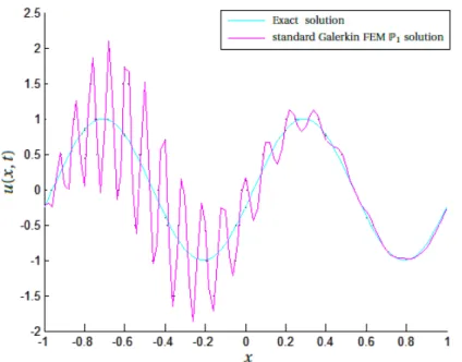
5.4 Exact and standard Galerkin FEMP1solution for the one-dimensional linear advection problem
at T = 0.4s. . . . 71
5.5 Exact, Galerkin and SUPG solutions at T = 0.4s. . . . 79
5.6 SUPG FEP1solution for different values ofα ∈ [0,1]. . . 80
5.7 Convergence in number of d.o.f. for different choices ofα. . . 82
5.8 UniformP2mesh of [a, b]. . . 83
5.9 Global shape functions for the space Vh2. . . 84
5.10 SUPG quadratic LagrangeP2FEM in conjunction with RK 2 for the 1D advection problem. . . . . 88
5.11 L2-error for the advection problem with the linear and quadratic Lagrange FEM. . . 90
6.1 An example of a B-spline patch in physical spaceΩ, parametric spaceΩ, and the reference ele-e mentΩ used to perform numerical integration. . . 95b 6.2 (a) SUPG B-spline linear solution for the advection problem (α = 0.1). (b) SUPG FEM P1for the advection problem (α = 0.1) at T = 0.4s. . . 101
6.3 SUPG quadratic B-spline solutions in conjunction with RK 2 for the advection problem. . . 102
6.4 Convergence rates in the L2-norm. . . 104
6.5 Error in the L2-norm of IGFEM and classical FEM vs. number of d.o.f. . . 105
7.1 L2-errors for the 1D advection problem using the DGFE method in conjunction with the RK method for a sinusoidal initial condition and Lax-Friedrichs flux. . . 118
7.2 Bézier decomposition (bottom) from a quadratic B-spline basis (top) by knot insertion. . . 120
7.3 IGDG solution of the 1D advection problem for quadratic (a), cubic (b) and quartic (c) basis and exact solution with 4 Bézier elements. RK 4 time discretization and Lax-Friedrichs flux were used. 123 7.4 L2-errors for the 1D advection problem with a sinusoidal initial condition, RK 2 and RK 4. . . 125
7.5 Convergence rates in IGDG method as a function of the Bernstein function is degree p for the finest grid. . . 125
7.6 Error in the L2-norm combining IGFEM, DGFEM, IGDG space discretization and explicit RK time integration. . . 127
8.1 An example of a B-spline patch in physical space, parametric space, and the parent element used to perform numerical integration. . . 133
8.2 ElementDe, its faces¡ Γe k ¢ k=1,...,4and the corresponding normals −→ne|Γek. . . 139
8.3 Analytical solution for the bi-dimensional advection problem, forNel= 4 × 4 at T = 0.5s. . . 141
8.4 Plots and contour plots of numerical results for bivariate quadratic Bernstein basis with (a)Nel= 4 × 4 patches and (b)Nel = 8 × 8 patches at T = 0.05s. . . 142
8.5 IGDG solution forNel= 8 × 8 patches for different degrees (p, q). . . 143
8.6 L2−error for the 2D advection problem using the IGDG method in conjunction with RK 4. . . 145
8.7 Contour plots of numerical results for bivariate quadratic Bernstein basis at T = 0.05s. . . 146
8.10 Contour plots of numerical results for bivariate quadratic Bernstein basis at T = 0.05s. . . 149
8.11 IGDG solutions for different bivariate degrees (p, q) forNel= 8 × 8. . . 150
8.12 L2−errors for the 2D advection problem using the IGDG method in conjunction with RK 4. . . . 152
9.1 Control point lattice for quadratic rectilinear grid (on the right) and curvilinear grid (on the left). 163 9.2 Rectilinear grid on the right and curvilinear grid on the left (4 × 4 elements). . . 164
9.3 Plots and contour plots of the exact pressure pex. . . 165
9.4 Plots and contour plots of uex. . . 165
9.5 Plots and contour plots of vanalytic. . . 166
9.6 Rectilinear patches. . . 166
9.7 Plots and contour plots of numerical results for bivariate quadratic Bernstein basis withNel = 4 × 4 patches at T = 0.1s. . . 168
9.8 Plots and contour plots of numerical results for bivariate quadratic Bernstein basisNel = 8 × 8 patches at T = 0.1s. . . 169
9.9 IGDG solution u for different degrees p forNel = 4 × 4 elements at T = 0.1s. . . 170
9.10 IGDG solution v for different degrees p forNel= 4 × 4 elements at T = 0.1s. . . 171
9.11 IGDG solution p for different degrees p forNel= 4 × 4 elements at T = 0.1s. . . 172
9.12 L2−error for the 2D acoustic problem using the IGDG method in conjunction with RK 4. . . 174
9.13 Curvilinear patches. . . 175
9.14 Plots and contour plots of numerical results for bivariate quadratic Bernstein basis withNel = 4 × 4 patches at T = 0.1s. . . 176
9.15 Plots and contour plots of numerical results for bivariate quadratic Bernstein basisNel = 8 × 8 patches at T = 0.1s. . . 177
9.16 IGDG solution u for different degrees p forNel = 4 × 4 elements at T = 0.1s. . . 178
9.17 IGDG solution v for different degrees p forNel= 4 × 4 elements at T = 0.1s. . . 179
9.18 IGDG solution p for different degrees p forNel= 4 × 4 elements at T = 0.1s. . . 180
L
IST OF
A
BBREVIATIONS
CAD Computer aided design.
CAGD Computer aided geometric design.
CAE Computer aided engineering.
CFL Courant-Friedrichs-Lewy.
DGM Discontinuous Galerkin method.
d.o.f. Degrees of freedom.
FDM Finite difference method.
FEM Finite element method.
FVM Finite volume method.
GLS Galerkin Least-Squares.
IGA Isogeometric analysis.
NURBS Non-uniform-rational B-spline.
ODE Ordinary differential equation.
PDE Partial differential equation.
PG Petrov-Galerkin.
PSPG Pressure-stabilizing Petrov-Galerkin.
RK Runge-Kutta.
L
IST OF
S
YMBOLS
p Degree of the polynomial approximation.
n Number of B-spline functions of degree p.
nG Number of nodes for Gauss quadrature methods.
ˇ
n Dimension of the time steps.
Nel Finite number of cells of DG method.
Nel Finite number of patchs of IGDG method.
N Dimension of the polynomial approximation.
Bpk k-th Bernstein polynomial of degree p in parameter space.
Bkp k-th Bernstein polynomial of degree p in physical space.
Ni ,p i -th B-spline function of degree p in parameter space.
Ni ,p i -th B-spline function of degree p in physical space.
Rip i -th NURBS function of degree p.
Cp Bézier curve of degree p.
Rp Rational Bézier curve of degree p.
S Bézier surface.
Cp B-spline curve of degree p.
S B-spline surface.
V B-spline volume.
Cp NURBS curve of degree p.
S NURBS surface.
Ξ Knot vector. Ω Physical space.
∂Ω Boundary of the domainΩ. e
Ω Parameter space. b
ωG The weights of nodes for Gauss quadrature methods.
v Test function.
ukh+ The field on the exterior of the element boundaryΓk.
ukh− The field on the interior of the element boundaryΓk.
CC F L Courant-Friedrichs-Lewy (CFL) number. c Advection velocity. − →c = (c x, cy) Velocity field. −
→n The outward unit normal. −
→ne The outer unit normal toΓe
of the elementΩe.
T Final time.
t0 Initial time.
τ SUPG stabilization parameter.
r Convergence rate.
M Mass matrix for theP1FEM.
M−1 Inverse of mass matrix.
MLs SUPG lumped mass matrix.
R Stiffness matrix for theP1FEM.
M1s Mass matrix for theP1SUPG-FEM.
M2s Mass matrix for theP2SUPG-FEM.
R1s Stiffness matrix for theP1SUPG-FEM.
R2s Stiffness matrix for theP2SUPG-FEM.
(MB)T Transpose of the mass matrix for the B-spline IGFEM.
RB Stiffness matrix for the B-spline IGFEM.
Q The matrix defined by the least square method. Mk Local mass matrix.
Rk Local stiffness matrix.
Mk Local mass matrix for IGDGM.
Rk Local stiffness matrix for IGDGM.
J The Jacobian matrix.
| J | Determinant of the Jacobian.
Je The elemental Jacobian matrix in the physical domainΩe.
∂xu =∂u∂x Partial derivative of u with respect to space x.
∂tu =∂u∂t Partial derivative of u with respect to time t .
⊗ Tensor product.
Ck The set of functions with k − th order continuous derivatives.
L Differential operator.
T Transformation of the parametric domain to the physical domain. T−1 Inverse of transformationT.
b
Fe Numerical flux in the patchΩe.
b fC E N Central flux. b fG Godunov flux. b fLF Lax-Friedrichs flux.
C
H
A
P
T
E
1
I
NTRODUCTION
H
Yperbolic systems of partial differential equations (PDEs) are mathematicalmod-els expressing the conservation of a physical quantity, as for instance mass, en-ergy, etc. They arise naturally from the conservation laws in physics. In particular, they describe a wide variety of phenomena that involve wave motion (such as acoustic, elastic, electromag-netic) or the advective transport of substances.
The wide range of applications of hyperbolic PDEs led to a very intense research activity in this field. It al-lowed to develop very early a set of numerical methods for accurate and computationally efficient approxi-mations to the solutions of such problems. There are three major families of methods which are widely used: the finite difference method, the finite volume method and the finite element method. These methods have proved to be extremely useful in modeling a broad set of phenomena. To keep this thesis self-contained, we briefly introduce each of these three methods in the context of hyperbolic PDEs.
Historically, the finite difference method (FDM) was the first method used to produce approximations of the solutions of hyperbolic PDEs. They were introduced by Euler in the 18t h century and represent the easiest method to solve problems on simple geometries [64]. The main idea of this method, is to replace the functional derivatives of the unknown by their FD approximations. The FDM is notable for the large variety of schemes that can be used to approximate a given PDE; e.g. explicit schemes (Forward Euler, Upwind, Lax-Friedrichs, Lax-Wendroff, Leapfrog, ...) and implicit schemes (Backward Euler, Crank-Nicolson,...) [88]. Although this method can be easily formulated and implemented, its application to problems with realis-tic geometries is rather cumbersome, thus making the method not very attractive for industrial problems. This fact urged the need for other methods with more flexibility, such as finite volume and finite element methods.
The finite volume method (FVM) can handle complex geometries which makes it more attractive for complex problems than the FDM. It is based on the conservative form instead of the differential form to estimate the values of unknown fields. We split the domain into grid cells and approximate the total integral over each grid cell, or actually the cell average, which is this integral divided by the volume of the cell. The links between the cell quantities in the FVM rely on the flux between neighbouring control volumes. This means that the FVM represents the flux of information within the structure of the mesh in a conservative way [56]. It allows the use of unstructured grids to handle complex geometries.
The finite element method (FEM), had its origins in the early 1960s and is nowadays the predominating method in analysis of elliptic or parabolic problems due to its flexibility to represent complex geometric domains and its strong theoretical basis. The idea consists in decomposing the domain into many small, “finite” elements which are defined by a set of nodal points and interpolating basis functions.
Although the FEM has been used widely in simulating many physical phenomena due to its flexibility to represent complex geometric domains, it is well known in the FE literature that numerical difficulties arise when solving hyperbolic PDEs. Indeed, when using the standard Galerkin FE method applied to hyperbolic PDEs, unwanted spurious (non-physical) oscillations (Gibbs phenomenon) are frequently detected in the numerical solutions. A cure to this drawback, widespread in the literature, is to add some "artificial" vis-cosity to a standard (unstable) numerical scheme. On the one hand, this artificial visvis-cosity should damp the oscillations but, on the other hand, it should not smear the numerical solution. In the late 1970s and early 1980s, a large number of so–called stabilized methods have been developed with different ideas [14] [32] [48]. This is achieved through the use of a Petrov-Galerkin formulation [35], where the test functions are modified such that they weight the upstream node more than the downstream node [17] [38]. Among them, the most popular, so called Streamline-Upwind Petrov–Galerkin (SUPG) method, was introduced by Brooks and Hughes. It was first proposed in the context of advection–diffusion equations and incompress-ible Navier–Stokes equations [14], and then extended to various other problems, e.g., coupled multidimen-sional advective–diffusive systems [44], first–order linear hyperbolic systems [49] or first–order hyperbolic systems of conservation laws [45].
Later, Galerkin/least-squares (GLS) has emerged as a generalization of the SUPG method, developed by Hughes et al. for convective transport problems [9] [30] [78], in which residuals of the equations in least-squares form are added to the standard Galerkin formulation. GLS has been successfully employed in a wide variety of applications where enhanced stability and accuracy properties are needed, including problems governed by Navier-Stokes and the compressible Euler equations in fluid mechanics [78].
We can also mention the pressure-stabilizing/Petrov-Galerkin (PSPG) [91] formulation which has been in-troduced for the stabilization of the Stokes equations [44] and incompressible Navier-Stokes equations [85].
troducing excessive numerical dissipation. Because its symptoms are not necessarily qualitative, excessive numerical dissipation is not always easy to detect. This concern makes it desirable to seek and employ stabi-lized formulations developed with objectives that include keeping numerical dissipation to a minimum. In these stabilized formulations, judicious selection of the stabilization parameter, which is almost known as
τ, plays an important role in determining the accuracy of the formulation. This yielded a significant amount
of attention and research [14] [30] [82] [83]. Typically this stabilization parameter involves a measure of the local length scale (also known as "element length") and other parameters such as the local Reynolds and Courant numbers. However, this stabilization parameter requires special attention, as it strongly depends on the problem under consideration and the chosen numerical method.
More recently, an alternative approach has emerged, the discontinuous Galerkin method (DGM), which shares some features with both the FVM and the FEM. Indeed, discontinuous polynomial functions are used and a numerical flux is defined at the interface between cells to reconstruct the solution. It has been proved very useful in solving a large range of problems. It was first introduced in 1973 by Reed and Hill for solving a time-independent linear hyperbolic equations [74] and, later on, it has been extended for solving nonlinear time-dependent equations. Subsequently, during the nineties of the last century the DGM experienced a series of developments by Cockburn and Shu, where numerical schemes for hyperbolic problems were pro-posed by combining DG approximation in space with Runge-Kutta time stepping strategies [18] [19] [21]. In fact, the DG method combines the advantages of stability of FVM and the accuracy of continuous FEM. Within each element, the solution is approximated by a polynomial of degree p ≥ 0 (as in FEM), while the continuity conditions applied to the solution are relaxed at the boundaries of elements (as in FVM), how-ever, motivated by the FVM, interface terms of the problem are approximated by a consistent, monotone and Lipschitz continuous numerical flux. This ensures that the scheme obtained is conservative, which does not hold in case of the classical FEM. In particular, the increasing interest in these kind of formulations are due to the following interesting features: they have good stability properties, they offer flexibility in the mesh construction (irregular meshes are admissible) and in the handling of boundary conditions (Dirichlet boundary conditions are weakly imposed), the accuracy is obtained by means of high-order polynomials within elements, without any regularity constraint at element interfaces. Furthermore, they are locally con-servative.
The fundamental difference between the DGM and the classical FEM relies on the continuity of basis functions. In comparison with the classical FEM, in DGM the basis functions are completely discontinuous across each element interface and they consist of local piecewise polynomials. Due to the fact that of basis function have compact support, integration can be achieved locally in each element. This simplifies the implementation of the method, since the mass matrix becomes block diagonal and the solution of a large system is avoided. In addition, the discontinuity across each element allows the use of different degrees of freedom in each element independently, which is not allowed in classical finite element method. Conse-quently, we can easily apply adaptivity strategies by increasing the degrees of freedom near phenomena of
interest to obtain better approximations to the solution.
As explained above, FEM decomposes the computational domain into many small, “finite” elements with simple shapes. A drawback is that with such elements there is usually no continuity higher than C0 be-tween elements. Even with higher-order polynomials it is difficult to guarantee C1continuity for arbitrarily shaped elements. With the advancement in design technology a more accurate and flexible handling of the geometry becomes necessary.
The design of free-from shapes by mathematical methods is a discipline, named computer-aided-design (CAD). It had its origins slightly later than the computer-aided-engineering (CAE). In fact, CAD is the use of computer technology for design: it allows the creation, modification, analysis and optimization of drawings and geometric modeling. The Bézier curve was the first method used to construct free-form curves and surfaces, and is named according to its inventor, Dr. Pierre Bézier. Bézier was an engineer in the Renault car company and developed this method in 1966. Actually, another French engineer, Paul de Casteljau at Citroën developed the same technology some years earlier. A further development to Bézier’s method were B-splines which provide more flexibility in the modeling of free-form curves and surfaces. Since 1975 non-uniform rational B-splines (NURBS) have been used in CAD programs, as a generalization of B-splines. The development of NURBS provided a technology that can exactly describe circular shapes (cylinders, spheres, etc.) which are basic elements in geometric modeling, but also allows very flexible modeling of free-form surfaces [43].
Today, there is a strong need for reducing the gap between CAD and FEM in terms of geometric represen-tations to gain in accuracy, flexibility and ease of interaction. A new form of analysis, named isogeometric analysis (IGA), tries to close this gap between CAD and FEA in such a way that both disciplines work on the same geometric models.
IGA is an extension of the FEM for solving PDEs. It was first introduced in 2005 by Hughes, Cottrell, and Bazilevs [43], and expanded in 2006 [24] in an effort to bridge the gap between FEM and CAD. The key idea is to use for analysis the same geometry used for geometric modeling. In fact, we use the same basis functions, which are used for the representation of the geometry in computer aided design (CAD) mod-els, also for the approximation of the solution of the PDE or the system of PDEs describing the physical phenomenon. The idea of using Bézier, B-splines or NURBS as basis functions is driven by the desire to in-tegrate CAD within FEM, and to have a strategy to replace a huge number of little cells (the FEs) by a reduced set of larger patches covering the entire domain. Moreover, there are several advantages of this approach over the FEM: easily control of the continuity, as Cp−1-continuity is obtained using p-th order NURBS, ex-act representation of the underlying NURBS geometry on the coarsest level of discretisation, as well as exex-act representation of the geometry as the mesh is refined [43].
IGA has been applied to a wide variety of different physical phenomena, including computational solid dynamics problems, computational fluid dynamics [23], coupled solid–fluid interaction problems [7] and the diffusion equation [37]. In last years, there has been an increasing interest in DG-IGA for the numerical solution of elliptic PDEs [40] [54] [69][95]. The advantages of the local approximation spaces without conti-nuity requirements that DG methods offer [5] [28] is thus employed to manage multi-patch computations.
emphasis is on the discontinuous Galerkin method, since it is considered as one of the most powerful and fastest growing methods with applications in various problems, not necessarily hyperbolic. The disconti-nuity of basis functions, which provides more flexibility in analysis, makes the method tedious however for handling realistic geometries from CAD.
The thesis is structured in four main parts: the first gives particular focus on the Bernstein and B-splines basis functions used in CAD. It is devoted to giving their definitions and basic properties. We present in the second and third parts the extension from classical analysis to IGA for the FE and DG methods, for the one-dimensional advection problem. In the last part, we deal with two one-dimensional hyperbolic problems by combining the IGA with the DG method. It should be mentioned, in all this work, that the discretization of equations in time is done by means of high-order explicit Runge-Kutta methods [18] [19] [34] [80].
More precisely, chapter 2 and chapter 3 provide a comprehensive introduction to the main ideas and properties of the Bernstein, B-splines and NURBS, which form the basis for the IGA. In the same context, an analysis of fitting B-spline curve and surface in the least squares sense is presented in chapter 4. The analysis is illustrated by examples of univariate and bivariate problems. Since IGA is an extension of FEM, we start by revisiting the original analysis framework in chapter 5, i.e. FEM. The need for stabilization is outlined and stabilization ideas based on the Petrov-Galerkin concept are discussed. We focus on the SUPG stabilization method and a special attention is given to the study of the stabilization parameterτ.
In chapter 6, the various computational procedures for IGA are reviewed in the context of FEM, by re-visiting the one-dimensional advection problem that is given in the previous chapter. While in this chapter we use B-splines (due to the simplicity of the domain) as a basis function, it is not hard to generalize it to other splines such as NURBS. Detailed comparisons between both IGA and classical FEM are discussed. In this context of IGA, we consider then the application of DG methods. Indeed, the major argument for us-ing DG methods lies with their ability to provide stable numerical methods for hyperbolic PDE problems, for which classical FEM is well known to perform poorly. Therefore, in chapter 7, we deal with one-dimensional advection problem by combining IGA method with the DG method. We note that the DG methodology is adopted at patch level, i.e., we employ the classical IGA within each patch, and employ the DG method across the patch interfaces. Moreover, a transformation of the B-spline basis is necessary to introduce dis-continuities at the interfaces, without modifying the geometry of the domain. The advantageous features of both IGA and DG method enable us to design a promising formulation.
With some adjustments, chapter 8 and chapter 9 are devoted to the study of two numerical examples in 2D. The advection problem is first presented, followed by the acoustic wave equations, where both systems are solved over several domains (Cartesian, linear and curvilinear).
Finally, in chapter 10 we end with some concluding remarks and outlooks. The results of the various studies performed are summarized and discussed, and ideas for future research are proposed.
L
Es systèmes d’équations aux dérivées partielles (EDPs) hyperboliques sont des mod-èles mathématiques permettant d’exprimer la conservation d’une quantité physique, comme par exemple la masse, l’énergie, etc. Ils découlent naturellement des lois de conservation en physique. En particulier, ils décrivent une grande variété de phénomènes impliquant le mouvement des ondes (acoustiques, élastiques, électromagnétiques) ou le transport advectif de substances. Le large éventail d’applications des EDPs hyperboliques a conduit à une activité de recherche très intense dans ce domaine. Cela a permis de développer un ensemble de méthodes numériques pour des approxi-mations précises et efficaces du point de vue du calcul des solutions à ces problèmes. Il existe trois grandes familles de méthodes qui sont largement utilisées: la méthode des différences finies (MDF), la méthode des volumes finis (MVF) et la méthode des éléments finis (MEF). Ces méthodes se sont révélées extrêmement utiles pour modéliser un large éventail de phénomènes. Pour garder cette thèse autonome, nous présen-tons brièvement chacune de ces trois méthodes dans le contexte des EDPs hyperboliques.Historiquement, la méthode des différences finies (MDF) était la première méthode utilisée pour pro-duire des approximations des solutions des EDPs hyperboliques. Elle a été introduite par Euler au 18ème siècle et représente la méthode la plus simple pour résoudre des problèmes sur des géométries simples [64]. L’idée principale de cette méthode est de remplacer les dérivées partielles de l’inconnu par leurs approxi-mations par des différences finis. La méthode DF est remarquable par la grande variété de schémas qui peu-vent être utilisés pour approcher une EDP donnée, par exemples, schémas explicites (Forward Euler, Up-wind, Lax-Friedrichs, Lax-Wendroff, Leapfrog, ...) et schémas implicites (Backward Euler, Crank-Nicolson, ...) [88]. Bien que cette méthode puisse être facilement formulée et mise en oeuvre, son application à des problèmes avec des géométries réalistes est assez lourde, ce qui rend la méthode peu attrayante pour les problèmes industriels. Cela a nécessité d’autres méthodes plus flexibles, telles que les méthodes de FV et d’EF.
La méthode des VF peut gérer des géométries complexes ce qui la rend plus attrayante que la méthode de DF pour les problèmes complexes. Elle est basée sur la forme conservative au lieu de la forme différen-tielle pour estimer les valeurs des champs inconnus. On divise le domaine en cellules et on approxime l’intégrale totale sur chaque cellule de la grille. Le liens entre les quantités de cellules dans la MVF dépen-dent du flux entre les volumes de contrôle voisins. Cela signifie que la MVF représente le flux d’informations dans la structure du maillage de manière conservative [56]. Elle permet l’utilisation de grilles non
struc-turées pour gérer des géométries complexes.
La méthode des éléments finis a ses origines au début des années 1960, elle est aujourd’hui la méth-ode prédominante dans l’analyse des problèmes elliptiques ou paraboliques en raison de sa flexibilité à représenter des domaines géométriques complexes et sa base théorique solide. L’idée consiste à décom-poser le domaine en plusieurs éléments «finis», définis par un ensemble de points nodaux et des fonctions de base interpolantes.
Bien que la MEF a été largement utilisée pour simuler de nombreux phénomènes physiques en raison de sa flexibilité à représenter des domaines géométriques complexes, il est bien connu dans la littéra-ture de la MEF que des difficultés numériques se posent lors de la résolution des EDPs hyperboliques. En effet, lors de l’utilisation de la méthode d’EF standard appliquée à de tels EDPs, des oscillations para-sites (non physiques) indésirables (phénomène de Gibbs) sont fréquemment détectées dans les solutions numériques. Un remède à cet inconvénient, répandu dans la littérature, consiste à ajouter une viscosité "ar-tificielle" à un schéma numérique standard (instable). D’une part, cette viscosité artificielle doit amortir les oscillations mais, d’autre part, elle ne doit pas entacher la solution numérique. À la fin des années 1970 et au début des années 1980, un grand nombre de méthodes dites stabilisées ont été développées avec des idées différentes [14] [32] [48]. Ceci est réalisé grâce à l’utilisation d’une formulation Petrov-Galerkin [35], où les fonctions test sont modifiées de telle sorte qu’elles pondèrent le noeud en amont plus que le noeud en aval [17] [38]. Parmi eux, la plus populaire, dite Streamline-Upwind Petrov-Galerkin (SUPG), a été introduite par Brooks et Hughes. Elle a été proposée d’abord dans le contexte des équations d’advection–diffusion et les équations de Navier–Stokes incompressible [14], puis elle a été étendue à divers autres problèmes, par exemples les systèmes advectifs–diffusifs multidimensionnels couplés [44], les systèmes hyperboliques linéaires du premier ordre [49], les systèmes hyperboliques de lois de conservation [45].
Plus tard, la méthode de Galerkin/moindres carrés (GLS) est apparue comme une généralisation de la méth-ode SUPG, développée par Hughes et al. pour les problèmes de transport convectif [9] [30] [78], dans laque-lle les résidus des équations des moindres carrés sont ajoutés à la formulation de Galerkin standard. La méthode GLS a été utilisée avec succès dans une large variété d’applications où des propriétés de stabilité et de précision améliorées sont nécessaires, y compris les problèmes régis par Navier-Stokes et les équations d’Euler compressible en mécanique des fluides [78]. On peut également citer la formulation de stabilisation de la pression/Petrov-Galerkin (PSPG) [91] introduite pour la stabilisation des équations de Stokes [44] et des équations de Navier-Stokes incompressibles [85].
procédé sans introduire de dissipation numérique excessive. Parce que les symptômes ne sont pas néces-sairement qualitatifs, une dissipation numérique excessive n’est pas toujours facile à détecter. Cette préoc-cupation rend la recherche et l’emploi de formulations stabilisées développées souhaitable avec des ob-jectifs tels que le maintien au minimum de la dissipation numérique. Dans ces formulations stabilisées, la sélection du paramètre de stabilisation, qui est souvent connu sous le nom deτ, joue un rôle impor-tant dans la détermination de la précision de la formulation. Cela a suscité beaucoup d’attention et de recherche [14] [30] [82] [83]. Ce paramètre de stabilisation implique généralement une mesure de l’échelle de longueur locale (également appelée «longueur d’élément») et d’autres paramètres tels que les nombres locaux de Reynolds et de Courant. Cependant, ce paramètre de stabilisation nécessite une attention parti-culière, car il dépend fortement du problème considéré et de la méthode numérique stabilisée choisie.
Plus récemment, une approche alternative a émergé, la méthode de Galerkin discontinue (MGD), qui partage certaines fonctionnalités avec MVF et MEF. En effet, des fonctions polynomiales discontinues sont utilisées et un flux numérique est défini à l’interface entre les cellules pour reconstruire la solution. Elle s’est avérée très efficace pour résoudre un large éventail de problèmes. Elle a été introduite pour la première fois en 1973 par Reed et Hill pour résoudre des équations hyperboliques linéaires indépendantes du temps [74] et plus tard, elle a été étendue pour résoudre des équations non linéaires dépendant du temps. Par la suite, au cours des années quatre-vingt-dix du siècle dérnier, Cockburn et Shu ont développé une série de sché-mas numériques pour les problèmes hyperboliques en combinant l’approximation de GD dans l’espace et les stratégies de Runge-Kutta pour la discrétisation temporelle [18] [19] [21].
En fait, la méthode de GD combine les avantages de la stabilité de la MVF et la précision de la MEF continue. Dans chaque élément, la solution est approchée par un polynôme de degré p ≥ 0 (comme dans la MEF), tandis que les conditions de continuité appliquées à la solution sont relâchées aux limites des éléments (comme dans la MVF), mais comme pour la MVF, les termes d’interface du problème sont approximés par un flux numérique continu, monotone et Lipschitz. Cela garantit que le schéma obtenu est conservatif, ce qui n’est pas le cas de la MEF classique. En particulier, l’intérêt croissant pour ce type de formulations est dû aux caractéristiques intéressantes suivantes: elles ont de bonnes propriétés de stabilité, elles offrent une flexibilité dans la construction du maillage (les maillages non structurés sont admissibles) et dans les conditions aux limites (les conditions aux limites de Dirichlet sont faiblement imposées), la précision est obtenue au moyen de polynômes d’ordre élevé dans les éléments, sans aucune contrainte de régularité aux interfaces d’éléments.
La différence fondamentale entre la MGD et la MEF classique repose sur la continuité des fonctions de base. En comparaison avec la MEF classique, dans la MGD, les fonctions de base sont complètement discontinues pour chaque interface d’élément et elles sont constituées de polynômes locaux par élément. Grâce au fait que des fonctions de base ont un support compact, l’intégration peut être réalisée localement dans chaque élément. Cela simplifie la mise en oeuvre de la méthode, puisque la matrice de masse devient diagonale en bloc et que la résolution d’un grand système est évitée.
De plus, la discontinuité entre chaque élément permet d’utiliser différents degrés de liberté dans chaque élément indépendamment, ce qui n’est pas autorisé dans la méthode des EF classiques. Par conséquent, nous pouvons facilement appliquer des stratégies d’adaptation en augmentant les degrés de liberté à prox-imité de phénomènes d’intérêt pour obtenir de meilleures approximations de la solution.
Comme expliqué ci-dessus, la MEF décompose le domaine en plusieurs éléments «finis» avec des formes simples. Un inconvénient est qu’avec de tels éléments, il n’y a généralement pas de continuité supérieure à C0entre les éléments. Même avec des polynômes d’ordre supérieur, il est difficile de garantir la continuité C1pour des éléments de forme arbitraire. Avec les progrès de la technologie de conception, une manipulation plus précise et flexible devient nécessaire.
La conception de les formes libres par des méthodes mathématiques est une discipline appelée con-ception assistée par ordinateur (CAO). Ses origines étaient un peu plus tardives que l’ingénierie assistée par ordinateur (IAO). En fait, la CAO est l’utilisation de l’informatique pour la conception: elle permet la création, la modification, l’analyse et l’optimisation de dessins et modélisations géométriques. Les courbes de Bézier ont été la première méthode utilisée pour construire une forme libre des courbes et des surfaces, elles sont nommées d’après leur inventeur Pierre Bézier. Bézier était ingénieur dans la société Renault au-tomobile et a développé cette méthode en 1966 [?]. En fait, un autre ingénieur français, Paul de Casteljau chez Citroën a développé la même technologie quelques années auparavant. Un autre développement de la méthode de Bézier concerne les B-splines qui offrent plus de flexibilité dans la modélisation des courbes et des surfaces de forme libre. Depuis 1975, les B-splines rationnelles non uniformes (NURBS) ont été util-isées dans les programmes de CAO comme une généralisation de B-splines. Le développement de NURBS a fourni une technologie capable de décrire exactement les formes circulaires (cylindres, sphères, etc.) qui sont des éléments de base de la modélisation géométrique, mais permet également une modélisation très flexible des surfaces à forme libre [43].
Aujourd’hui, il existe un fort besoin de réduire l’écart entre la CAO et la MEF en termes de représen-tations géométriques pour gagner en flexibilité, précision et en facilité d’interaction. Une nouvelle forme d’analyse, appelée analyse isogéométrique (AIG), tente de combler cet écart entre la CAO et la MEF de telle manière que les deux disciplines fonctionnent avec les mêmes modèles géométriques.
L’AIG est une extension de la MEF pour la résolution des EDPs. Elle a été introduite pour la première fois en 2005 par Hughes, Cottrell et Bazilevs [43], et développé dans 2006 [24] pour tenter de combler le fossé entre la MEF et la CAO.
les modèles de conception assistée par ordinateur (CAO), également pour l’approximation de la solution des EDPs ou des systèmes des EDPs décrivant le phénomène physique. L’idée d’utiliser Bézier, B-splines ou NURBS comme fonctions de base est motivée par le désir d’intégrer la CAO dans la MEF, et d’avoir une stratégie pour remplacer un grand nombre de petites cellules (les EF) par un ensemble réduit de plus gros patches couvrant tout le domaine. De plus, cette approche présente plusieurs avantages par rapport à la MEF: contrôle facile de la continuité, car la continuité Cp−1est obtenue en utilisant une NURBS de degré p, représentation exacte de la géométrie en utilisant une NURBS au niveau de discrétisation le plus grossier, ainsi que la représentation exacte de la géométrie lorsque le maillage est affiné [43].
L’AIG a été appliquée à une grande variété de phénomènes physiques, y compris la dynamique des flu-ides computationnelle [23], les problèmes d’interaction couplé fluide-structure [7] et l’équation de diffusion [37]. Au cours des dernières années, la méthode de GD dans le cadre IG a manifesté un intérêt croissant pour la solution numérique des EDPs elliptiques [40] [54] [69][95]. Les avantages des espaces d’approximation locaux sans exigences de continuité offerts par les méthodes de GD [5] [28] sont alors utilisés pour gérer les calculs multi-patch.
L’objectif principal de cette thèse est d’étudier l’utilisation des AIG pour résoudre certains problèmes hyperboliques. En particulier, nous décrivons la méthode de Galerkin continue et discontinue en utilisant la base des B-splines. Un accent particulier est mis sur la méthode de GD, car elle est considérée comme l’une des méthodes les plus efficaces et à la croissance la plus rapide, avec des applications dans divers problèmes, pas nécessairement hyperboliques. Les discontinuités des fonctions de base, qui offrent une plus grande souplesse d’analyse, rendent cependant la méthode délicate pour gérer des géométries réal-istes à partir de la CAO.
La thèse est divisée en quatre parties principales: la première met l’accent sur les fonctions de base de Bernstein et B-splines utilisées en CAO. Elle est consacré à donner leurs définitions et propriétés de base. Nous présenterons dans la deuxième et troisième parties l’extension de l’analyse classique à l’AIG pour les méthodes d’EF et GD, pour le problème d’advection unidimensionnel. Dans la dernière partie, nous traitons des problèmes hyperboliques en deux dimensions en combinant l’AIG avec la méthode de GD. Il convient de mentionner que dans tout ce travail, la discrétisation des équations dans le temps se fait au moyen de méthodes de Runge-Kutta explicites d’ordre élevé [18] [19] [34] [80].
Plus précisément, les deuxième et troisième chapitres fournissent une introduction complète aux prin-cipales idées et propriétés des fonctions Bernstein, B-splines et NURBS, qui constituent la base de l’AIG. Dans le même contexte, la construction des courbes B-spline et des surfaces au sens des moindres carrés est présentée au quatrième chapitre. L’analyse est accompagnée d’exemples de problèmes univariés et bi-variés.
L’AIG étant une extension de la MEF, nous commençons par revoir le cadre de l’analyse originale au cin-quième chapitre, à savoir: la MEF. Le besoin de stabilisation est souligné et les idées de stabilisation basées sur le concept Petrov-Galerkin sont discutés. Nous nous concentrons sur la méthode de stabilisation SUPG et une attention particulière est accordée à l’étude du paramètre de stabilisationτ.
Au niveau du sixième chapitre, les différentes procédures de calcul pour l’AIG sont passées en revue dans le contexte de la MEF, en revisitant le problème d’advection unidimensionnel qui est présenté dans le chapitre précédent. Dans ce chapitre nous utilisons les B-splines (en raison de la simplicité du domaine) comme fonctions de base, il n’est pas difficile de le généraliser pour d’autres splines telles que les NURBS. Des comparaisons détaillées entre l’AIG et la MEF classiques sont discutées. Dans ce contexte de l’AIG, nous considérons alors l’application des méthodes GD. En effet, l’argument majeur pour utiliser les méthodes de GD réside dans leur capacité à fournir des méthodes numériques stables pour les EDPs hyperboliques, pour lesquelles la MEF classique est bien connue pour ses performances médiocres. Par conséquent, au septième chapitre, nous traitons le problème d’advection unidimensionnelle en combinant la méthode de l’AIG avec la méthode de GD. Nous notons que la méthodologie de GD est adoptée au niveau du patch, c’est-à-dire que nous employons l’AIG classique dans chaque patch et utilisons la méthode de GD à travers les interfaces de patch. De plus, une transformation de la base B-spline est nécessaire pour introduire des discontinuités aux interfaces, sans modifier la géométrie du domaine. Les caractéristiques avantageuses des deux méthodes AIG et GD nous permettent de concevoir une formulation prometteuse.
Avec quelques ajustements, les huitième et neuvième chapitres sont consacrés à l’étude de deux ex-emples numériques en 2D, le problème d’advection est d’abord présenté, suivi par les équations d’ondes acoustiques, où les deux systèmes sont résolus sur plusieurs domaines (cartésien, linéaire et curviligne).
Enfin, au niveau du dernier chapitre, nous terminons avec quelques remarques et perspectives finales. Les résultats des différentes études réalisées sont résumées et discutées et des idées de recherches futures sont proposées.
C
H
A
P
T
E
2
B
ÉZIER
C
URVES
B
Ézier curves are parametric curves commonly used in computer graphics and re-lated fields. They are named after their inventor, Dr. Pierre Bézier, an engineer from the Renault car company who developed in the early 19600s a curve formulation foruse in shape design. The main interest of Bernstein-Bézier patches is that they lend to an easy geometric understanding of the underlying mathematical concepts. Some basic properties and a brief discussion of Bernstein polynomials and Bézier curves [8] are presented in the present chapter.
2.1 Bernstein basis
Bézier curves are expressed in terms of Bernstein polynomials which where introduced by Sergei Bern-stein in order to formulate a constructive proof of the Weierstrass approximation theorem.
Definition 2.1.1. (Univariate Bernstein)
The Bernstein polynomials of degree p over the interval [0, 1] are defined explicitly by: Bpk(ζ) = Ckpζk(1 − ζ)p−k ∀ k = 0, ..., p,
with the binomial coefficients Cpkgiven by:
Cpk= p! k!(p−k)! if 0 ≤ k ≤ p, 0 otherwise.
An example of constant, linear, quadratic and cubic Bernstein polynomials are presented in Fig. 2.1:
Figure 2.1: Constant, linear, quadratic and cubic Bernstein polynomials.
Definition 2.1.2. (Multivariate Bernstein)
In order to define Bernstein basis in higher dimensions, we make use of the tensor product construction. Let p = (p1, p2, ..., pd) be a vector inNd. The d -dimensional Bernstein polynomials are defined by a tensor product
of d univariate Bernstein polynomials with possibly different degrees p = (p1, p2, ..., pd) and multi-indices
k = (k1, k2, ..., kd). Therefore, ∀ζ = (ζ1,ζ2, ...,ζd) ∈ [0,1]dwe get: Bkp(ζ) = Bk1 p1(ζ1) ⊗ B k2 p2(ζ2) ⊗ ... ⊗ B kd pd(ζd).
The bivariate Bernstein polynomials are illustrated in Fig. 2.2 for the linear, quadratic and cubic cases.
2.2 Properties of the Bernstein polynomials
The Bernstein polynomials Bpkof degree p, have several important properties [50]: 1. Recursion
The Bernstein polynomials satisfy the following recursion relation: for p > 0, we have: Bp0(ζ) = ¡1 − ζ¢p if k = 0, Bpk(ζ) = ¡1 − ζ¢Bp−1k (ζ) + ζBk−1p−1(ζ) if k = 1,..., p − 1, Bpp(ζ) = ζp if k = p. Proof. ∀1 ≤ k ≤ p − 1, we have ¡1 − ζ¢Bk p−1(ζ) = ¡1 − ζ¢Cp−1k ζk¡1 − ζ¢ (p−1)−k = Cp−1k ζk¡1 − ζ¢p−k = ¡p − 1¢! k!³¡p − 1¢ − k´!ζ k¡1 − ζ¢p−k = ³p − k p ´ Bkp(ζ). Similarly, ξBk−1 p−1(ζ) = ζCk−1p−1ζk−1¡1 − ζ¢ (p−1)−(k−1) = Cp−1k−1ζk¡1 − ζ¢p−k = ¡p − 1¢! ¡k − 1¢!³¡p − 1¢ − ¡k − 1¢´!ζ k¡1 − ζ¢p−k = ¡ k p¢B k p(ζ). Therefore, ¡1 − ζ¢Bk p−1(ζ) + ζBp−1k−1(ζ) = ¡ p − k p ¢B k p(ζ) + ¡ k p¢B k p(ζ) = Bpk(ζ). ■
2. Non-negativity
The Bernstein polynomials are positive everywhere in [0, 1].
Bpk(ζ) ≥ 0 ∀ζ ∈ [0, 1] 0 ≤ k ≤ p.
Note that the Lagrange interpolating polynomials, commonly used as basis for the numerical solution of partial differential equation (PDE), do not satisfy this property.
3. Partition of unity
The Bernstein polynomials of degree p forms a partition of unity, that is:
p X k=0 Bkp(ζ) = 1 ∀ζ ∈ [0, 1]. Proof. p X k=0 Bpk(ζ) = p X k=0 Ckpζk¡1 − ζ¢p−k= ³ ξ + (1 − ξ)´p= 1. ■ 4. Unique maximum
The Bernstein polynomial Bkphas a unique maximum atζ =kp on [0, 1].
5. Symmetry
The Bernstein polynomials are symmetric in the sens:
Bpk(1 − ζ) = Bpp−k(ζ) ∀0 ≤ k ≤ p.
6. Basis for polynomials of degree less or equal p
The Bernstein polynomials of degree p form a basis for the space of polynomials of degree less than or equal to p.
7. Degree elevation
Any Bernstein polynomial of degree less than p can be expressed as a linear combination of Bernstein polynomials of degree p. In particular, any Bernstein polynomial of degree p − 1 can be written as a linear combination of Bernstein polynomials of degree p.
Bk (ζ) = µ p − k¶ Bk(ζ) + µ k + 1¶ Bk+1(ζ).