Chaos and predictability of homogeneous-isotropic turbulence

HAL Id: hal-01636012

https://hal.archives-ouvertes.fr/hal-01636012

Submitted on 16 Nov 2017

HAL is a multi-disciplinary open access

archive for the deposit and dissemination of

sci-entific research documents, whether they are

pub-lished or not. The documents may come from

teaching and research institutions in France or

abroad, or from public or private research centers.

L’archive ouverte pluridisciplinaire HAL, est

destinée au dépôt et à la diffusion de documents

scientifiques de niveau recherche, publiés ou non,

émanant des établissements d’enseignement et de

recherche français ou étrangers, des laboratoires

publics ou privés.

Chaos and predictability of homogeneous-isotropic

turbulence

G Boffetta, Stefano Musacchio

To cite this version:

G Boffetta, Stefano Musacchio. Chaos and predictability of homogeneous-isotropic turbulence.

Phys-ical Review Letters, American PhysPhys-ical Society, 2017. �hal-01636012�

G. Boffetta1,2 _{and S. Musacchio}3

1

Department of Physics and INFN, Universit`a di Torino, via P. Giuria 1, Torino, Italy

2

Institute of Atmospheric Sciences and Climate (CNR), Torino, Italy

3

Universit´e Cˆote d’Azur, CNRS, LJAD, Nice, France

We study the chaoticity and the predictability of a turbulent flow on the basis of high-resolution direct numerical simulations at different Reynolds numbers. We find that the Lyapunov exponent of turbulence, which measures the exponential separation of two initially close solution of the Navier-Stokes equations, grows with the Reynolds number of the flow, with an anomalous scaling exponent, larger the one obtained on dimensional grounds. For large perturbations, the error is transferred to larger, slower scales where it grows algebraically generating an “inverse cascade” of perturbations in the inertial range. In this regime our simulations confirm the classical predictions based on closure models of turbulence. We show how to link chaoticity and predictability of a turbulent flow in terms of a finite size extension of the Lyapunov exponent.

The strong chaoticity of turbulence does not spoil com-pletely its predictability. Such apparent paradox is re-lated to the hierarchy of timescales in the dynamics of turbulence which ranges from the fastest Kolmogorov time to the slowest integral time.

Ruelle argued many years ago that the growth of in-finitesimal perturbations in turbulence is ruled by the fastest timescale [1]. This leads to the prediction that the Lyapunov exponent is proportional to the inverse of the Kolmogorov time, and hence it increases with the Reynolds number. Turbulent flows at high Re are there-fore strongly chaotic [2]. Nonetheless, the time that it takes for a small perturbation to affect significantly the dynamics of the large scales is expected to be of the or-der of the slow integral time [3]. The ratio between these extreme timescales increases with the Reynolds number and therefore allows a finite predictability time to coex-ists with strong chaos [4]. This is evident from every-day experience: while the Kolmogorov time of the atmo-sphere (in the planetary boundary layer) is a fraction of a second [5] the weather is predictable for days.

The study of the predictability problem in turbulence dates back to the pioneering works of Lorenz [3] and of Leith and Kraichnan [6, 7]. The main idea of those stud-ies is that a finite perturbation at a given scale in the inertial range of turbulence grows with the characteristic time at that scale. Therefore, while an infinitesimal per-turbation is expected to grow exponentially fast, finite perturbations grow only algebraic in time, making the predictability of the flow much longer. These ideas were applied to the predictability of decaying turbulence [8], two-dimensional turbulence [9, 10] and three-dimensional turbulence at moderate Reynolds numbers [11].

In this letter we investigate, on the basis of high-resolution direct numerical simulations, chaos in homogeneous-isotropic turbulence by measuring the growth of the separation between two realizations start-ing from very close initial conditions. In the limit of in-finitesimal separation we compute the leading Lyapunov exponent of the flow (rate of exponential growth of the

separation [12]) and we find that it increases with the Reynolds number, but surprisingly faster than what pre-dicted on dimensional grounds [1] and what observed in low-dimensional models of turbulence [13]. For larger separation we observe the transition to an algebraic growth of the error, in agreement with the predictions of closure models [7]. Finally, we discuss the relation between chaoticity and the predictability time of turbu-lence (defined as the average time for the perturbation to reach a given threshold) in terms of the finite-size gener-alization of the Lyapunov exponents.

We consider the dynamics of an incompressible velocity field u(x, t) given by the Navier-Stokes equations

∂tu+ u · ∇u = −∇P + ν∆u + f , (1)

where P is the pressure field and ν is the kinematic vis-cosity of the fluid. The term f represents a mechanical forcing needed to sustain the flow. In the following we will present results in which the forcing is a determin-istic forcing with imposed energy input [14, 15]. The Navier-Stokes is solved numerically by a fully parallel pseudo-spectral code in a cubic box of size L at resolu-tion N3 _{with periodic boundary conditions in the three}

directions. The main parameters of the simulations are reported in Table I and further details are found in the Supplementary Material.

In presence of forcing and dissipation, the turbulent flow reaches a statistically steady state in which the en-ergy dissipation rate ε = νh(∂αuβ)2i is equal to the

input of energy provided by the forcing (brackets indi-cate average over the physical space). The turbulent state is characterized by a Kolmogorov energy spectrum E(k) = Cε2/3_k−5/3_{. The kinetic energy E =}R _{E(k)dk =}

(1/2)h|u|2

i fluctuates around a constant mean value, which defines the typical intensity of the large scale flow U = (2E/3)1/2_{. The integral time is defined as T = E/ε}

and the integral scale is L = U T .

We performed a series of simulations at increasing Reynolds number Re = U L/ν. In order to ensure that the viscous range is resolved with the same accuracy in

2 all the simulations, the increase of Re as been achieved

by increasing the resolution N and reducing the viscosity in order to keep fixed kmaxη = 1.7, where kmax= N/3 is

the maximum resolved wavenumber and η = (ν3

/ε)1/4 _is

the Kolmogorov scale.

N Re E U L η τη λ

1024 8224 0.700 0.683 4.78 0.005 0.063 2.72 512 3062 0.678 0.672 4.56 0.01 0.10 1.39 256 1170 0.665 0.666 4.43 0.02 0.16 0.76 128 434 0.643 0.655 4.21 0.04 0.25 0.44 TABLE I: Parameters of the simulations. For all the simula-tions the energy input is ε = 0.1, and the box size is L = 2π. N is the grid resolution, Re = U L/ν the Reynolds number, E

the kinetic energy, U = (2E/3)1/2 is the large-scale velocity,

L = U E/ε the integral scale, η = (ν3

/ε)1/4 _{the Kolmogorov}

scale, τη= (ν/ε)1/2the Kolmogorov time and λ the Lyapunov

exponent.

For the study of chaos and predictability we are in-terested in measuring the growth of an uncertainty in the velocity field. Starting from an initial velocity fields u1(x, 0) in the stationary turbulent state, we generate a

perturbed velocity field u2(x, 0), obtained by adding to

the reference field a small white noise (the relative am-plitude of the perturbation is O(10−4

). We consider very small initial perturbations in order to guarantee that the separation between the two realizations is along the most unstable direction in the phase space when the error en-ters in the non-linear stage and therefore we do not con-sider the effect of the distribution of the initial error on the predictability of the flow [16]. The two realizations of the velocity field are then simultaneously evolved in time according to (1). For each resolution, we performed an average over several independent realizations.

A natural measure of the uncertainty is the error en-ergy E∆(t) and the error energy spectrum E∆(k, t),

de-fined on the basis of the error field δu ≡ (u2− u1)/

√ 2 as E∆(t) = Z ∞ 0 E∆(k, t)dk = 1 2h|δu(x, t)| 2 i . (2) With the normalization coefficient 1/√2 we have E∆= E

for completed uncorrelated fields.

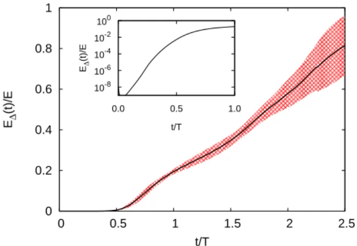
Figure 1 shows the time evolution of the error en-ergy E∆ for the simulation at the highest Re, averaged

over an ensemble of 10 independent realizations. In the initial stage the error grows exponentially as E∆(t) =

E∆(0) exp(L2t) (see inset of Fig. 1) where L2is the

gen-eralized Lyapunov exponent of order 2 [17]. At later times we observe a regime of linear growth of the error E∆(t) ≃ εt. The growth rate displays large fluctuations

as the error approaches its saturation value E∆(t) ≃ E.

This is due to the fluctuations of the kinetic energy asso-ciated to the dynamics of the large scales, which occurs

0 0.2 0.4 0.6 0.8 1 0 0.5 1 1.5 2 2.5 E∆ (t)/E t/T 10-8 10-6 10-4 10-2 100 0.0 0.5 1.0 E∆ (t)/E t/T

FIG. 1: Error energy E∆(t) growth for the simulation at

N = 1024. The error energy is averaged over 10 different realizations (black line). The fluctuations of the error energy within one standard deviation from the mean are represented by the shaded area. Inset: The initial exponential growth of the error.

on the same time scale of the saturation of the error. It is worth to notice that the late regime of saturation of the error might display a non-universal behavior with respect to the forcing mechanism. As an example, the deterministic force used in our study is proportional to the large-scale velocity. At late times, when the error has significantly affected the large scales, the force acting on the two fields u1and u2becomes different. This could

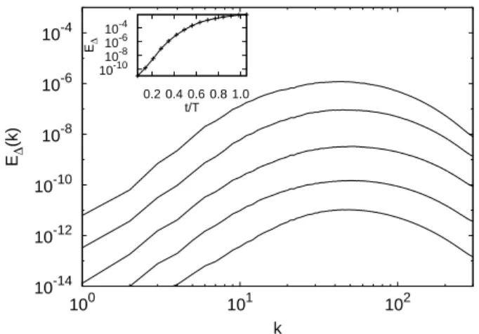
in-duce a faster saturation of the error with respect to other forcing mechanism which enforce large-scale correlations. During the initial stage of exponential growth the er-ror energy spectrum E∆(k, t) is peaked at wavenumbers

around the dissipation range k ≃ kη ≃ 1/η and grows

exponentially in self similar way, as shown in Fig. 2. At later times, the error propagates to lower wavenum-bers and the error spectrum develops a scaling range E∆(k) ∼ k−5/3 (see Fig. 3). At each time it is possible

to identify the error wavenumber kE(t) at which the

er-ror energy spectrum have reached a given fraction α ≃ 1 of the energy spectrum E∆(kE, t)/E(kE) = α. The two

velocity fields u1and u2can be then assumed to be

com-pletely decorrelated at scales smaller than 1/kEand still

correlated at larger scales.

The transition from the exponential growth to the lin-ear growth of E∆ occurs when the two fields are

com-pletely decorrelated on the dissipative scales, that is when kE ≃ kη . The idea, originally proposed by Lorenz [3],

is that the time that it takes to decorrelate completely the two fields at a given scale ℓ ≃ 1/k within the in-ertial range is proportional to the turnover time of the eddies at that scale τℓ∼ ε−1/3ℓ2/3[18]. This leads to the

dimensional prediction

10-14 10-12 10-10 10-8 10-6 10-4 100 101 102 E∆ (k) k 10-10 10-8 10-6 10-4 0.2 0.4 0.6 0.8 1.0 E∆ t/T

FIG. 2: The spectrum of the error E∆(k, t) at times t/T =

0.07, 0.14, 0.21, 0.28, 0.35 (from bottom to top) in the linear phase for the simulation at N = 1024 averaged over 10

inde-pendent realizations. Inset: The error energy E∆ as a

func-tion of time in semilogarithmic plot.

10-6 10-4 10-2 100 100 101 102 E(k) k 101 102 103 1 5 kE L t/T

FIG. 3: The spectrum of the error E∆(k, t) at times t/T =

0.42, 0.56, 0.70, 0.84, 1.1, 1.4, 1.8, 2.1 (dashed lines, from bot-tom to top) compared with the stationary energy spectrum E(k) (solid line) for simulations at N = 1024 averaged over 10 independent realizations. The dotted line represents the

Kol-mogorov scaling k−5/3_{. Inset: The error wavenumber k}

E as

a function of time (crosses), compared with the dimensional

scaling kE∼t3/2(dotted line).

for the evolution of the error wavenumber, which is con-firmed by our numerical finding (see inset of Fig. 2).

Equation (3) provides an estimation of the predictabil-ity time TP that an infinitesimal error takes to

contami-nate a given wavenumber k, Tp(k) = Aε−1/3k−2/3[7, 19]

where the dimensionless coefficient A depends on the threshold α (and possibly on the Reynolds number). In our simulation at Re = 8516 we measure A = 12 for α = 0.5 to be compared with the value A = 10 obtained from early studies with closure models in the limit of infinite Re [7].

Integrating the error spectrum with the ansatz E∆(k, t) = 0 for k < kE(t) E∆(k, t) = E(k) for k > kE(t)

and using the dimensional scaling (3), one obtains the prediction for the linear growth of the error energy:

E∆(t) = Gεt . (4)

The value of the dimensionless constant G measured in the simulation at Re = 8516 is G = 0.45 ± 0.05, not far from what obtained by the test field model closure G = 0.23 [7].

As already discussed, in the early stage the perturba-tion can be considered infinitesimal and therefore grows exponentially as shown in the inset of Fig. 1. This is the signature of the chaotic nature of the flow and the pre-dictability is characterized by the Lyapunov exponent λ. On dimensional grounds the Lyapunov exponent can be assumed to be proportional to the inverse of the fastest time-scale of the flow, i.e., the Kolmogorov timescale τη = (ν/ε)1/2 [1]. Since the ratio between τη and the

integral timescale T increases with the Reynolds number as T /τη ∼ Re1/2 one has the prediction that the

Lya-punov exponent is proportional to the square root of the Reynolds number:

λ ≃ τη−1≃ T −1

Re1/2. (5)

Therefore the predictability time TPfor infinitesimal

per-turbations vanishes in the limit of large Re.

The dimensional prediction (5) is obtained under the assumption of self-similarity of the velocity field with Kolmogorov scaling exponent h = 1/3 [18] For a generic exponent h ∈ (0 : 1) one has λ ≃ τ−1

η ≃ T −1

Reβ _with

β = (1−h)/(1+h). Averaging over the multifractal spec-trum D(h) of the exponents h allows to take into account for the intermittency corrections and this gives β = 0.459 [13, 20].

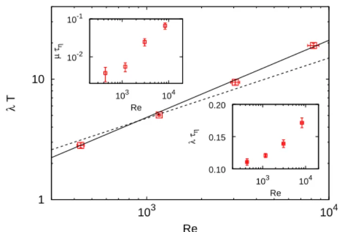
We have computed the Lyapunov exponent λ by mea-suring the average rate of logarithmic divergence of two close realizations, a standard method in the study of dy-namical systems [17, 21, 22], for the simulations at dif-ferent Reynolds numbers (see Table I). Interestingly, we find that the Lyapunov exponent increases with Re faster than the dimensional prediction (5), as shown in Fig. 4. Fitting the measured values with a power law λT ≃ Reβ

gives the exponent β = 0.64 ± 0.05. It is remarkable that the measured deviation with respect the dimensional pre-diction β = 0.5 is opposite with respect the predicted cor-rection due to intermittency. Our findings suggest that the dimensional estimate of the Lyapunov exponent as the inverse Kolmogorov time is not accurate to charac-terize the chaoticity of a turbulent flow. The inset of Fig. 4 shows that indeed the quantity λτη increases with

Re.

Since the Lyapunov exponent is an average quantity, it is interesting to investigate its fluctuations and their dependence on Re. We have therefore measured the vari-ance µ of the distribution of the finite-time Lyapunov

4 1 10 103 104 λ T Re 0.10 0.15 0.20 103 104 λ τ η Re 10-2 10-1 103 104 µ τ η Re

FIG. 4: Lyapunov exponents λ as a function of Re (squares).

The solid line represents the best fit scaling λT ≃ Re0.64

while the dashed line is the dimensional scaling λT ≃ Re1/2.

Lower inset: The Lyapunov exponents λ compensated with

the Kolmogorov time scale τηas a function of Re. Upper inset:

The Lyapunonv variance µ compensated with the Kolmogorov

time scale τηas a function of Re.

exponents, a standard measure of the fluctuations in a chaotic system [12, 17] (see also the Supplementary Ma-terial). The results, plotted in Fig. 4, shows that also µτη increases with Re and faster than the Lyapunov

ex-ponent (a fit gives µT ≃ Re1.2 _{although the errors here}

are large).

The connection between predictability and chaoticity in turbulent flows can be extended also to finite pertur-bations, of the order of the velocities of the inertial range, by means of the finite size Lyapunov exponents (FSLE) Λ(δ). The FSLE has been introduced to measure the chaoticity of systems with many characteristic time scales [4, 20]. It is defined in terms of the average time Tr(δ)

that it takes for a perturbation of size δ to grow by a fac-tor r, as Λ(δ) = ln(r)/hTr(δ)i (where the average is now

over different realizations). We remind that performing averages at fixed times is not equivalent to averaging at fixed error size. The latter procedure has revealed to be more effective in intermittent systems, in which scaling laws can be affected by strong fluctuations of the error (as in Fig. 1).

In the limit δ → 0 the FSLE recovers, by definition, the usual Lyapunov exponent, i.e. limδ→0Λ(δ) = λ [20].

For finite errors, Λ(δ) measures the average growth rate of the uncertainty of size δ. Following the idea of Lorenz [3] that a perturbation of size δ ∼ uℓ within the inertial

range of turbulence grows with the local eddy turnover time τℓ∼ ε−1/3ℓ2/3∼ ε−1u2ℓ, one obtains the prediction

[20]

Λ(δ) ≃ εδ−2

. (6)

In Figure 5 we show the FSLE as a function of the error δ for three values of Re. For small δ the FSLE

10-1 100 101 10-3 10-2 10-1 100 Λ ( δ ) T δ/U 10-2 10-1 100 10-3 10-2 10-1 100 101 λ ( δ )/ λ δ/δ*

FIG. 5: Finite-size Lyapunov exponents Λ(δ) (FSLE) as a function of the velocity uncertainty δ for N = 1024 (red squares) N = 512 (blue circles) N = 256 (purple

trian-gles). The values of the Lyapunov exponents λ are also

shown (dashed lines). Black solid line represents the scaling

Λ(δ) ∼ δ−2_{. Inset: The FSLE Λ(δ) rescaled by the Lyapunov}

exponents λ as a function of the rescaled uncertainty δ/δ∗_.

approaches the constant value Λ(δ) ≃ λ, while in the in-ertial range we observe the dimensional scaling (6). The crossover between the two regimes is expected to occur at δ∗

≃ (ε/λ)1/2_{. Rescaling the error δ with δ}∗ _{and Λ(δ)}

with λ we find a good collapse of the two regimes of infinitesimal and finite errors, as shown in the inset of Fig. 5. Figure 5 also shows that the crossover range be-tween the two regimes increases with Re. One possibile explanation for this long crossover is that the transition between the two regimes involves the dynamics of ed-dies which are at the border between the inertial and the dissipative scales, in the so-called intermediate dissipa-tive range [18]. The extension of this range is known to grow with the Reynolds number, and this could cause the broadening of the crossover regime for the FSLE.

Remarkably, Figure 5 shows that in the scaling range Λ(δ) ∼ δ−2_{the error growth rate Λ becomes independent}

both on the Reynolds number and on the values of the Lyapunov exponent. The independence of the FSLE in the scaling range on the value λ observed for infinitesimal errors provides a clear explanation of how in turbulent flows it is possible to observe the coextistence of long predictability time at large scales and strong chaoticity at small scales.

In conclusion, we studied the chaotic and predictability properties of fully developed turbulence by simulating two realizations of the velocity field initially separated by a very small perturbation. At short times the separation increases exponentially as a consequence of the chaoticity of the flow. Finite perturbations increase linearly in time, as predicted by dimensional arguments, and the time for the perturbation to affect a wavenumber k in the inertial range is proportional to ε−1/3_k−2/3_.

The Lyapunov exponent is found to grow with the Reynolds number faster than what predicted by dimen-sional argument and intermittency models and, as a con-sequence, the product λτη grows with Re. This indicates

that the strong, intermittent fluctuations of turbulence at small scales give diverse contributions on different ob-servable. In addition to the interest for many applica-tions, turbulence is a prototypical example of system with many scales and characteristic times. Our results on the chaoticity of turbulence and its dependence on the num-ber of active degrees of freedom are therefore of general interest for the study of extended dynamical systems.

The Authors gratefully acknowledge support from the Simons Center for Geometry and Physics, Stony Brook University, where part of this work was performed. The COST Action MP1305, supported by COST (European Cooperation in Science and Technology) is acknowledged. Numerical simulations have been performed at Cineca within the INFN-Cineca agreement INF17 fldturb.

[1] D. Ruelle, Phys. Lett. 72A, 81 (1979). [2] R. G. Deissler, Phys. Fluids 29, 1453 (1986). [3] E. N. Lorenz, Tellus 21, 289 (1969).

[4] G. Boffetta, M. Cencini, M. Falcioni, and A. Vulpiani, Phys. Rep. 356, 367 (2002).

[5] J. R. Garratt, The atmospheric boundary layer, vol. 416 (Cambridge University Press, 1992).

[6] C. E. Leith, J. Atmos. Sci. 28, 145 (1971).

[7] C. E. Leith and R. H. Kraichnan, J. Atmos. Sci. 29, 1041 (1972).

[8] O. M´etais and M. Lesieur, J. Atmos. Sci. 43, 857 (1986). [9] S. Kida, M. Yamada, and K. Ohkitani, J. Phys. Soc.

Japan 59, 90 (1990).

[10] G. Boffetta and S. Musacchio, Phys. Fluids 13, 1060 (2001).

[11] S. Kida and K. Ohkitani, Phys. Fluids A 4, 1018 (1992). [12] E. Ott, Chaos in dynamical systems (Cambridge

Univer-sity Press, 2002).

[13] A. Crisanti, M. Jensen, A. Vulpiani, and G. Paladin, Phys. Rev. Lett. 70, 166 (1993).

[14] L. Machiels, Phys. Rev. Lett. 79, 3411 (1997).

[15] A. G. Lamorgese, D. A. Caughey, and S. B. Pope, Phys. Fluids 17, 015106 (2005).

[16] K. Hayashi, T. Ishihara, and Y. Kaneda, Statistical The-ories and Computational Approaches to Turbulence p. 239 (2013).

[17] M. Cencini, F. Cecconi, and A. Vulpiani, Chaos: from

simple models to complex systems, vol. 17 (World

Scien-tific, 2010).

[18] U. Frisch, Turbulence (Cambridge Univ. Press, 1995). [19] J. I. Cardesa, A. Vela-Mart´ın, S. Dong, and J. Jim´enez,

Phys. Fluids 27, 111702 (2015).

[20] E. Aurell, G. Boffetta, A. Crisanti, G. Paladin, and A. Vulpiani, Phys. Rev. Lett. 77, 1262 (1996).

[21] G. Benettin, L. Galgani, and J. Strelcyn, Phys. Rev. A

14, 2338 (1976).

[22] G. Benettin, L. Galgani, A. Giorgilli, and J. Strelcyn, Meccanica 15, 9 (1980).