CAM~RI-zL~ 33, Mr;,hS~l',i¢it;UE'f TS, U.S.A.
-
ACU
T'IS
SA.
ANALYSIS OF HIGH-FREQUENCY
IONOSPHERIC SCATTERING
GORAN EINARSSON0
A
9
C'p7
TECHNICAL REPORT 400 NOVEMBER 15, 1962
MASSACHUSETTS INSTITUTE OF TECHNOLOGY
RESEARCH LABORATORY OF ELECTRONICSCAMBRIDGE, MASSACHUSETTS
The Research Laboratory of Electronics is an interdepartmental laboratory in which faculty members and graduate students from numerous academic departments conduct research.
The research reported in this document was made possible in part by support extended the Massachusetts Institute of Tech-nology, Research Laboratory of Electronics, jointly by the U.S. Army (Signal Corps), the U.S. Navy (Office of Naval Research), and the U.S. Air Force (Office of Scientific Research) under Signal Corps Contract DA 36-039-sc-78108, Department of the Army Task 3-99-20-001 and Project 3-99-00-000; and in part by Signal Corps Contract DA-SIG-36-039-61-G14.
Reproduction in whole or in part is permitted for any purpose of the United States Government.
MASSACHUSETTS INSTITUTE OF TECHNOLOGY RESEARCH LABORATORY OF ELECTRONICS
Technical Report 400 November 15, 1962
A COMMUNICATION ANALYSIS OF HIGH-FREQUENCY IONOSPHERIC SCATTERING
G6ran Einarsson
Submitted to the Department of Electrical Engineering, M. I. T., January 15, 1962, in partial fulfillment of the requirements for the degree of Master of Science.
(Manuscript received March 15, 1962)
Abstract
A communication scheme for random multipath channels is investigated. During predetermined intervals the transmitter sends a sounding signal that the receiver uses to predict the behavior of the channel during the intermediate time when communication is performed. It is assumed that the channel varies slowly, and that the additive noise in the receiver is low.
The possibility of representing a multipath channel as a time-variant filter is inves-tigated. A sampling theorem for linear bandpass filters is derived, and the results that can be expected when it is used to represent a single fluctuating path with Doppler shift are discussed.
The prediction operation is essentially linear extrapolation: a formula for the mean-square error is derived and compared with optimum linear prediction in a few cases. Calculations on actual data from ionospheric scattering communication show that the method is feasible and give good correspondence with the theoretical results.
Under the assumption that the receiver makes decisions on each received waveform separately, and that there is no overlap between successive waveforms, the optimum receiver is derived. It consists mainly of a set of matched filters, one for each of the possible waveforms. The predicted value of the channel parameters is used in weighting the output from the matched filters to obtain likelihood ratios.
The eventual practical value of such a communication system is still an open ques-tion, but this formulation provides means for dealing with random multipath channels in a way suitable for mathematical analysis.
TABLE OF CONTENTS
INTRODUCTION 1
1. 1 History of the Problem 1
a. The Probability-Computing Receiver 1
b. Other Research 3
c. Discussion 5
1.2 The Ionosphere 7
1.3 Communication System to Be Considered 8
II. A MODEL OF SCATTERING MULTIPATH 11
2. 1 Introduction 11
2.2 Linear Network Representation 11
a. Sampling Theorem and Delay-Line Model 11
b. Example 1 13
c. The Ionosphere as a Tapped Delay Line 13
d, Modulated Random Processes 16
2.3 A Physical Model of the Ionosphere 18
III. METHODS OF PREDICTION 20
3. 1 Introduction 20
3. 2 Pure Prediction 20
a. Last-Value Prediction 20
b. Maximum Likelihood Prediction 21
c. Tangent Prediction 22
d. Examples 24
e. Conclusions 30
3.3 Smoothing and Prediction 31
a. Regression-Line Prediction 32
b. Minimization of the Mean-Square Error 33
3.4 Computations on Ionospheric Data 35
a. Source of Data 35
b. Presentation of the Data 35
c. Results 37
d. Discussion 40
CONTENTS
IV. THE RECEIVER
4. 1 Introduction
4. 2 Complex Waveforms
4. 3 Computation of Probabilities a. The "Likelihoods"
b. Distribution for the Sufficient Statistics U and V c. The Weighting Function Wi(U, V)
d. The Receiver Block Diagram 4.4 Discussion
Appendix A Sampling Theorem for Time-Variant Filters
Appendix B Modulated Random Processes
Appendix C Regression-Line Prediction
Appendix D The Weighting Function W(U, V)
Acknowledgment References iv 42 42 42 45 45" 48 53 56 57 59 63 66 71 74 75
I. INTRODUCTION 1. 1 HISTORY OF THE PROBLEM
a. The Probability Computing Receiver
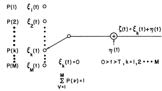
The problem of detecting known signals disturbed by additive noise can be stated as follows (see Fig. 1). The transmitter has M possible waveforms, each of duration T. It sends one of them, say k(t) with probability P(k). The signal is disturbed by additive white Gaussian noise ir(t) and the received signal is 'k(t) = k(t) + (t). We assume that the receiver knows the form of the M possible waveforms and we want it to determine which one was sent. All of the information that the receiver needs for that purpose is contained in the set of a posteriori probabilities P(k(t)/A(t)), k = 1, .. ., M. It is clear that a receiver that computes this for all k and chooses the index which gives the largest probability minimizes the probability of making a mistake. Using Bayes' equality we can write
(1) P(k(t)/t)) =
v=l1
where p denotes probability density. Since independent of the index k and the P(k) was need only compute the conditional probability the noise is Gaussian, p((t)/Ak(t)) is going to sible to show that
P(I)
Cl(t)
P(2)
0P(k)
P(M)
2
(t)
k
( t) CM(t)the denominator of (1) is a constant assumed to be known, the receiver density p(r (t)/Sk(t)) for each k. Since
be a Gaussian density and it is
pos-0 0 0 0
(t)
=
k(t)+7(t )
··
~k(t
):=° 0 0 kO>t
>T , k =
,2
*
M
M
Z
P(v):I
V=I
Fig. 1. Signals disturbed by white Gaussian noise,
1 P(k) p(S(t)/Sk OM
---p(v) p(w)/t V
(0)
Fig. 2. Optimum receiver for additive white Gaussian noise. 2T N (Pk- 1 / 2 Skk) p(=(t)/k(t)) = const. e k (2) where Pk =T Jk(t) , (t) dt (3) 1 T 2 Skk =T & k(t) dt (4)
and No is the noise power per unit bandwidth. We see that the receiver has to evaluate
the correlation integral Pk between the received waveform and each possible transmitted waveform. This can be done, for instance, by matched filters. The receiver then takes into account the possible difference in signal energy and signal probabilities, P(k), and decides which waveform was actually sent. (See Fig. 2.)
The receiver of Fig. 2 performs these desired operations; in this report we use the term "optimum receiver" for a device that computes the probability density p(r,(t)/gk(t)) or a monotonically related function in order to make its decision. We have stated the problem as a one-shot problem but for white Gaussian noise it is clear that the performance of the receiver is still optimum whenever the transmitted waveforms are statistically independent of each other. A more detailed presentation of the optimum receiver for additive noise has been given by Fano.9
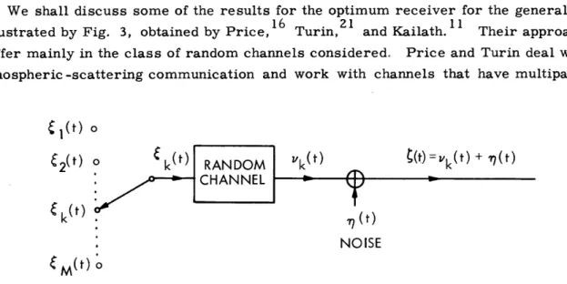
Let us now consider a more general problem in which the transmitted signal is per-turbed by a random channel in addition to the white noise. (See Fig. 3.) By the term random channel, we mean a linear time varying filter whose variation is guided, in gen-' eral, by a multidimensional random process. The problem of determining the function of the probability computing receiver in this case has been studied by several authors. In the next paragraph we review some of the results obtained.
2
b. Other Research
We shall discuss some of the results for the optimum receiver for the general case illustrated by Fig. 3, obtained by Price, Turin, and Kailath. Their approaches differ mainly in the class of random channels considered. Price and Turin deal with ionospheric -scattering communication and work with channels that have multipath
l(t) o 62(t) 0
Ek
( t ) RANDOM Vk(t) (t)=vk(t) + ( t )k(t)
.)CHANNEL~,(t)
NOISE (M(t) oFig. 3. Signals disturbed by a random channel plus noise.
structure. Kailath considers a very general channel for which the statistics need not even be stationary. All three authors assume that the receiver has complete knowledge about the statistics of the channel and the additive noise, which are assumed to be sta-tistically independent of each other. The decision is made on each waveform separately. This means that the receiver is, strictly speaking, optimum only for the "one -shot case," since it does not exploit the fact that successive output waveforms may be statistically dependent. Finally, it is assumed that both the transmitter and the receiver have the
same time standard.
Price considers a random channel that consists of a number of paths with known delay. Each path has a stationary narrow-band Gaussian process associated with it. The different paths are assumed to be statistically independent. If we send an unmod-ulated carrier through this channel, we receive Z(t) = yc(t) cos wot -Ys(t) sin wot, where Yc(t) and Ys(t) are lowpass, independent, Gaussian processes with zero mean and identi-cal autocorrelation. The first-order statistics of the envelope of Z(t) are then Rayleigh distributed and the phase distribution is flat. See, for instance, Davenport and Root7 for a presentation of the narrow-band Gaussian process. For this type of channel, Price obtains the optimum receiver in open form. The operations that the receiver should perform are given in the form of integral equations. For the special case of a single path and input signals that are constant or vary exponentially with time, they derive in detail the structure of the probability computing elements. The case of very low
signal-to-noise ratio is also considered in some detail.
Turin works with a similar multipath model. The channel is represented by a num-ber of independent paths each of which is characterized by a path-strength ai, a phase
shift Oi, and a delay Ti . The channel is so slowly varying that these quantities can be
considered as constants during the transmission time T. The strength and phase shift of the paths are assumed to be represented by a constant vector plus a vector with Ray-leigh distribution for amplitude and completely random phase. Since the Rayleigh dis-tribution is characterized by a single parameter, say i., each path is determined by four quantities: the amplitude ai and the phase 6i of the constant vector and -i and Ti.
For the case ai = 0, Turin's channel is the same as Price's for slowly varying paths. Turin considered the following cases: the receiver knows all four channel parameters; the receiver does not know 6 (in which case it assumes completely random phase); T
and 6 are not known and the receiver assumes 6 to be completely random and T to have
a flat distribution within two time limits. It is interesting to notice that the optimum receiver under most of the conditions above computes the correlation integral between the received signal and the possible transmitted signals delayed according to the path
delay Ti. The terms corresponding to different paths are then combined, by using the
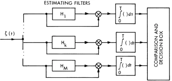
known statistical parameters of the paths, to obtain the probabilities p((t)/tk(t)). Kailath has a much more general random channel than Price and Turin. His only restriction is that the channel be Gaussian, i. e., that the output vk(t) sampled at arbi-trary instants of time gives a multidimensional Gaussian distribution for all values of k. When vk(t) has zero mean for all t, Kailath derives an optimum receiver that looks
like Fig. 4. He shows, also, that the estimating filters Hk can be interpreted as a mean-square-error estimator of vk(t) when k was actually sent. The same result was obtained earlier by Price for the random filter consisting of a single path. We see that when the receiver does not know the channel exactly, it estimates, on the basis of its statistical knowledge, what the received signal should look like before the noise was added if a par-ticular signal was sent. It then crosscorrelates this estimate with the actually received
signal to obtain a quantity that is monotonically related to the a posteriori probabilities
1CTIkAATIKIr- CIl TEDC
Fig. 4. Optimum receiver for zero mean Gaussian random channel plus noise.
ESTIMATING FILTERS
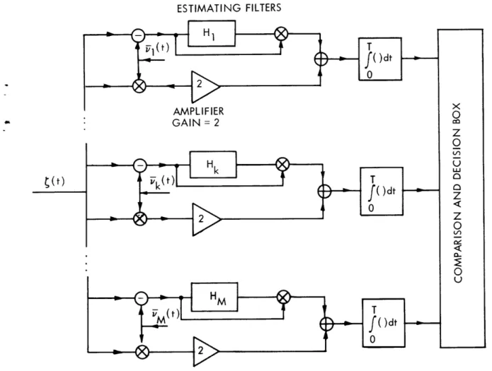
Fig. 5. Optimum receiver for Gaussian random channel plus noise (General Case).
It is important to notice that this interpretation of the optimum receiver is valid only if vk(t) has zero mean. When this is not the case, Kailath gives the receiver structure of Fig. 5 in which vk(t) is the mean of vk(t) (already known by the receiver under the assumption that a particular k was used). The gain factor 2 on the amplifier shows that the receiver puts greater weight on the part of the signal that it knows exactly than on the part it has to estimate.
Kailath considers a very general case and he obtains very general results. His esti-mating filters are given in the form of limits of very large inverted matrices. It is hard to say much more than that it is possible to instrument them as linear time-variant filters.
c. Discussion
Price and Turin consider specific multipath models that are more or less applicable to ionospheric -scattering communication, while Kailath considers a more general model.
The thing that they have in common is the assumption that the receiver has complete
5
statistical knowledge of the channel. To obtain this statistical knowledge, we have to measure the parameters of the channel, but since additive noise is present, we cannot do this exactly. To build an estimator that is optimum in some sense, we need to know in advance some of the statistical parameters that we want to measure. To some extent this is a closed circle, but we can, at least in prin-ciple, start guessing the statistical parameters that we need and then construct an optimum estimator on the basis of this guess. This, we hope, gives us a better estimate of the statistics and we can use this as a priori information to construct a better estimator, and so on.
Perhaps a more serious problem to consider is whether or not the channel is sta-tionary. For a statistical description to be at all useful, the channel has to be at least
quasi-stationary; that is, we can consider it stationary during the time in which we are using it for communication. If the properties of the channel change and we have to make repetitive measurements of the statistical parameters and then change our
optimum receiver according to these measurements, we have a painfully elaborate scheme.
As we have pointed out, the theoretical work on optimum receivers has been done under the assumption that the receiver makes its decision on each waveform separately. If the channel is varying very fast, so that the disturbances from one transmitted signal to the next are essentially independent, this is clearly the best that we can do. If, on the other hand, the channel changes only slowly during the transmission of a signal, we are not using all of the available information about the channel. Since the receiver tries to circumvent the fact that it does not know exactly what the channel was by making an estimate on the basis of the received waveform, it can clearly do better in the case of
slow variations by extending this estimate over consecutive signals.
The RAKE receiver described by Price and Green17 is an attempt to use the ideas of optimum receivers for combatting random multipath in a practical case. Two orthog-onal waveforms are used, and the receiver makes an estimate of the path structure of the channel by crosscorrelating the sum of the two possible signals with the received
signal. It is possible to do this, since the signals have nonoverlapping spectra. The time constant of the correlator is greater than the duration of the signal, and the receiver is thus operating over more than one signal at a time. The estimate of the path structure is then used to correct the received signal before the decision is made.
If the channel is nonstationary and the receiver is faced with the problem of obtaining statistical knowledge of the channel, it is perhaps just as easy for the receiver to try to measure the channel itself. For such measurements to be useful, the channel must vary slowly, so that it does not change much between transmitted signals. Price1 5 and
-Turin2 0 have discussed the possibility of estimating the instantaneous state of the chan-nel by using a sounding waveform known to the receiver. In this report we are going to outline a communication procedure that is based on this idea for a slowly varying multipath medium.
6
1. 2 THE IONOSPHERE
The propagation of radio waves via ionized layers in the upper atmosphere has been considered for more than half a century and an established theory exists. For a certain incident angle there is a maximum usable frequency (MUF) below which the wave is returned to earth by a process of gradual refraction. Since there exist several layers at different altitudes and, in addition, the wave can make several hops, it is clear that we are dealing with a multipath medium. Other things that contribute to this structure are the splitting of the wave into an ordinary wave and an extraordinary wave because of the earth's magnetic field, and the possibility of a ground wave. The mathematical theory of radio waves in the ionosphere can be found in Budden.6
A different kind of propagation mode, called scattering, has received considerable attention during the last decade. If there are irregularities in the ionosphere, they act
as oscillating electric dipoles when exposed to an electromagnetic wave, and in this way energy can return to the earth. The possibility of using scattering for long distance communication was pointed out in a paper by Bailey and others. The scattered field is comparatively weak, but it provides means for communication beyond the horizon with frequencies higher than the MUF.
In a paper written in 1948, Ratcliffe pointed out that if we assume that the down-coming wave is scattered by many "scattering centra," each scattering the same amount of power and completely randomly distributed in space, we are going to receive a narrow-band Gaussian process if we send up an unmodulated carrier. Moreover, if the scattering centra move in the same fashion as molecules in a gas, that is, if the line-of-sight velocity has a Gaussian distribution, the power spectral density of the down-coming wave is Gaussian and of the form
1 -(f-f ) /2cr 2 W(f) a - e , (5) where 2f V o o c
with Vo the rms velocity of the scattering centra, and f the frequency of the incident
wave. We can state these properties in another way. The downcoming wave can be expressed in the form
Z(t) = V(t) cos (Zirft+d(t)). (6)
The envelope V(t) has a Rayleigh distribution of the form
2 t V 2 t 2a 2 tp(V t) e Vt > 0 (7) Or 7
If we look at the quadrature components
Ys(t) = V(t) sin +(t) and yc(t) = V(t) cos (t)
we see that they are independent Gaussian processes with identical autocorrelation of Gaussian form.
We notice that these statistics correspond to the assumptions in Price's work about the optimum receiver.
If, in this idealized case, we have a specular component of amplitude A in the down-' coming wave, the distribution for the envelope takes the form
V2+A2 -t
V 2 /AV \
p(V ) t e I 0 ° vt o (8)()t
ar
See Davenport and Root7 for a derivation. This kind of distribution was first considered by Ricel9 in his classical paper of 1945, and we use the name "Rician distribution" for it. This was the type of statistics which Turin used in his work.
Ratcliffe's model of the scattering process is, of course, too simple to represent the physical phenomena that occur. More complicated theories have been presented by Booker and Gordon, Villars and Weisskopf, and others, but they all seem to lead to the Rayleigh distribution for the envelope when there is no specular component.
Measurements of the statistics of scattered radio waves have been presented by many authors. A brilliant and extensive study of ionospheric transmission at medium fre-quency (543 kcps) has been made by Brennan and Phillips.4 They computed the distribu-tion of the envelope of the received wave and made a test to determine whether or not it had a Rician or Rayleigh distribution. The result was perhaps somewhat disappointing; in more than half of the 200, or more, cases analyzed, they determined "no fit." The computed correlation functions for the envelope took many widely different forms, and it was not possible to assign any general shape to them.
The ionospheric scattering has multipath structure if we have different scattering regions with different transmission times. Most of the measurements reported have been made with a continuous wave, and very little is known about the statistics of the multipath structure. It should be of interest to know, among other things, more about how many paths are present, if the paths are statistically independent, and the nature of variation in the delay between paths. Another effect that needs to be studied is the Doppler effect that a steadily moving scattering region should produce. Some work in this area is presented in a thesis by Pratt, and other work is being done at Lincoln Laboratory, M. I. T.
1.3 THE COMMUNICATION SYSTEM TO BE CONSIDERED
On the basis of the theoretical investigations that have been reviewed we are going to outline a possible scheme for communication over random multipath channels. The
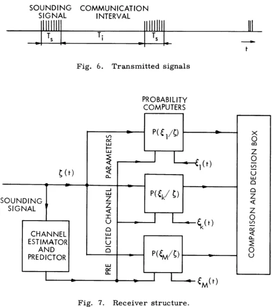
SOUNDING SIGNAL
11111111
COMMUNICATION INTERVAL1111ll 1
111
iITs
L
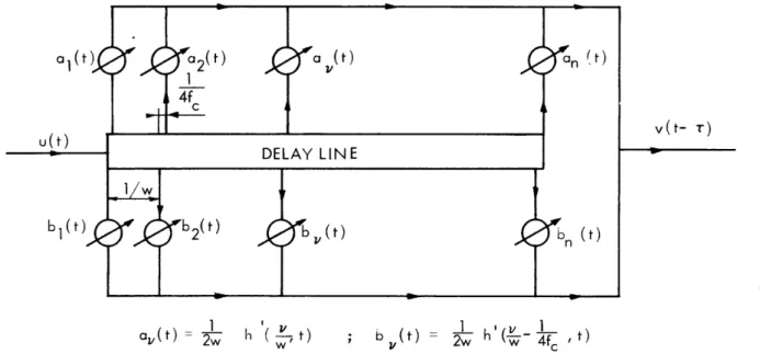
ToSI t Fig. 6. Transmitted signalsPROBABILITY COMPUTERS
Fig. 7. Receiver structure.
receiver is probably not optimum in any sense, but it should work well, at least, under certain conditions.
We assume that the transmitter sends information during the time intervals of length Ti. Between these intervals, it sends a predetermined signal of length Ts from which
the receiver tries to obtain knowledge about the multipath medium. In the particular case considered here, this sounding signal consists of a number of short pulses; with these as a basis the receiver tries to predict the behavior of certain channel parameters during the next Ti seconds. The receiver uses this predicted knowledge about the chan-nel when it makes its decision of what was sent. See Figs. 6 and 7.
The prediction operation that is to be used is simply linear extrapolation. See Fig. 8. During the Ts seconds the receiver knows that channel parameter exactly apart from
additive noise. It determines a straight line that fits the curve in a least-square sense, and uses this line as predicted value of the parameter for the next Ti seconds, during
9
(ADDITIVE NOISE
f
SLOWLY VARYING CHANNEL PARAMETER AI T S PREDICTED VALUE I PREDICTION T. ERROR tFig. 8. Prediction operation.
which information is being sent. This procedure contains a smoothing operation that is necessary because of the additive noise, but does not use any statistical knowledge about the process and it should work just as well (or badly) in a nonstationary case as in a stationary one.
This procedure is clearly based on some assumptions: that it is possible to char-acterize the multipath medium with a number of slowly varying parameters; that the signal-to-noise ratio is high enough, and so on. Measurements made by Group 34 at Lincoln Laboratory seem to indicate that it should be possible to use the outlined pro-cedure for ionospheric scattering HF communication, and we are going to investigate it for that kind of channel.
We first consider the problem of representing the ionospheric scattering with a model channel whose parameters are simple to measure and predict, and which is still capable of representing the channel closely enough for practical purposes. Section II deals with the prediction operation and some calculations are carried out with actual ionospheric data. In Section IV the derivation of the receiver structure is given.
10
II. A MODEL OF SCATTERING MULTIPATH 2. 1 INTRODUCTION
To work our problem we need a model of the communication channel. First, we con-- sider the representation of ionospheric scattering by a timecon--variant linear network. The
assumption that the receiver makes repetitive measurements of the channel emphasizes - the need for a simple model with a limited number of parameters to be determined. The
linear-network approach has the advantage of being quite general, but it seems to lead to unnecessary complexity when it is used to represent multipath or frequency shift. The model that we chose to use is discussed in the last part of this Section and it is based mainly on physical facts about scattering communication.
2.2 LINEAR NETWORK REPRESENTATION a. Sampling Theorem and Delay-Line Model
If we consider a communication link having wave propagation in a time-variant but linear medium, we can characterize the channel as a filter with an impulse response changing with time. See Fig. 9. The response function h(y, t) contains all information about the channel that we can possibly need, but it can be extremely complicated. For electromagnetic wave propagation, for instance, with signals of different frequencies traveling according to different physical mechanisms, it would be hard to visualize any over-all impulse response. In a practical case, in general, we use bandlimited signals in a narrow region, and we are not interested in such a complete description a knowl-edge of h(y, t) should provide. If our transmitted signal u(t) is bandlimited in the band
w~f~f w
fc - w2 f + fw it can be shown that (see Appendix A) that we can write the received signal as
v(t) h(y t)u(t-y)dy v() = h0 ' ( y t ) u(t-y)dy
-co
u(t) BANDLIMITTED: f w<
ifl__
<
f +w Fig. 9. Time-variant linear filter.11
I
-v(t)= 2w h'( ,t) u(t- ) _ (
n n
2w ( n t)
(t-2w
_
where the circumflex denotes Hilbert transforms, and h'(y, t) is related to h(y, t) by the formula A-6 of Appendix A. If our signal u(t) is narrow-band (i. e., fc >>w), we can get an easy expression for the Hilbert transform.
Write u(t) in terms of its quadrature components
u(t) = uc(t) cos 2Zrfct - us(t) sin 21Tfct. (10)
Taking the Hilbert transform (for instance, by passing it through the filter in Fig. A-2), we get
(t) = uc(t) sin 2fct + us(t) cos 2fct.
Since uc(t) and us(t) are slowly varying lowpass functions, we have
c
( 4fc )
(1 1)
and analogously h'(y, t) h' 4f,
.
The summations in Eq. 9 go from -oo to +oo, but in most practical cases h' (, t) goes to zero rapidly enough for In
I
large, so we can introduce a suitable delay T and represent formula (9) by the delay line in Fig. 10.It should be pointed out that the particular form of the response function for the time-variant network that we have chosen is not the only possible one. Our treatment of the
a(t) = 2w (-t) h ,(t)
· I~~~~~~~~~~
Fig. 10. Delay-line model for narrow-band functions.
12
_
subject is very similar to that of Kailath12 to which we refer for other possible repre-sentations.
b. Example 1
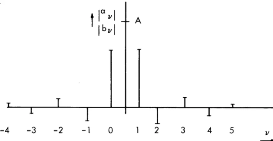
As an example we derive the delay-line model for the simple channel in Fig. 11, composed of a time delay 6 and a frequency shift Af. As is shown in Appendix A, we obtain
h'(y,t) = A2w sine [w(y-6)] cos [2Tr(fc(y-6)+Aft)+$] (12)
A
h'(y, t) = A2w sine [w(y-6)] sin [2rr(fc(y-6)+Aft)+$] (13)
If we choose fc and w so that fc = NW, where N is an integer, the tap gains in Fig. 10 become
av(t) = h' ( ,t = A sine (v- cos (2rAft+O) (14)
b (t) = w,t) = A sine (--) sin (2TwAft+O). (15)
Here, 0 = 9 + 2rfc6. The tap gain functions are simple sinusoids with frequency given by the frequency shift. The magnitude of av or bv as a function of the tap number v is
1 given in Fig. 12 for
2w-2w'
e ( 2rAft + ) f>o H (jf,t) = A e-i2fS .( 2Aft +)
Fig. 11. Filter with delay and frequency shift.
c. The ionosphere as a tapped delay line
Measurements of ionospheric radio-wave propagation indicate that the ionosphere can be considered a linear medium, at least in the sense that nonlinear effects are of second order. For communication purposes, the signal bandwidth is always much smaller than the carrier frequency. It should therefore be possible to represent the
13
t
Ia
v
I bvI T,
T
1 I - AT
T I I -4 -3 -2 -1 0 1 2 3 4 5 vFig. 12. Amplitude of the tap gain functions for the filter illustrated in Fig. 11. ionosphere over a certain frequency band with the tapped delay line shown in Fig. 10.
If we decide to use the delay-line model, the question arises whether or not we can easily measure the tap gain functions. To determine the response function of a time-variant filter, we need to know the output signal corresponding to a number of succeeding input signals. This is difficult to perform for an ionospheric propagation link, since it is hard to establish the same time scale at both transmitter and receiver. The sampling theorem in formula (9) is in terms of samples of a high-frequency waveform. In prac-tice it is inconvenient to instrument this directly, and some kind of demodulator is gen-erally used in the measurement system.
Taking these matters into consideration, we investigate a particular way of meas-uring the characteristics of the ionosphere. We are interested in the frequency band
w w A
f - w f f + w. As a sounding signal we use a lowpass function g(t) with a band-width wg > w2 and multiply it by a carrier frequency to get a narrow-band function. At the receiver we use a quadrature demodulator to provide information about the phase, as well as the amplitude of the received signal. We assume that the receiver knows the time at the transmitter apart from a constant value 6 and that the local oscillator in the demodulator is timed to the frequency fc + AfE. See Fig. 13.
To get a feeling for what we can expect if we perform such measurements, let us consider replacing the ionosphere by the filter in Fig. 12, except that A and are slowly varying with time (slowly compared with ) to get a fading effect. We can con-sider this as a model of a slowly varying path with Doppler shift. We send a sequence of g(t):s, spaced T seconds apart, and record the corresponding output from the demod-ulator. Since the parameters A and are slowly varying, we can use the results from Example 1,and the tap gains that we determine are of the form
a(t) = av A(t) cos [2rAft+O(t)]
(16) bV(t) = b A(t) sin [2wrAft+O(t)].
14
With the simple channel structure that we have assumed, the outputs from the demod-ulator us and uc are copies of g(t), spaced T seconds apart, but with varying amplitude. (See Fig. 13.) If we determine the amplitude for each transmission, the outputs can
QUADRATURE DEMODULATOR ig(t) -f 0(t) tVC(t) T
I-J
T T J t _- -_ N 4.WAVEFORMS FOR ASINGLE PATH WITH DOPPLER SHIFT
Fig. 13. Measurements of the ionosphere.
15 - · . o
)
·~ ~
i wI
--- - . ____ t -.1 -K___
Ij
be considered as samples, t seconds apart, of the time functions
Vc(t) = A(t-TE) cos [(2Tr(Af+fE)(t+(t-T)+(t-TE)] (17)
Vs(t) = A(t-TE) sin [(2rr(Af+AfE)(t- (t-TE)]. (18)
It is thus possible to determine the tap gain functions apart from a time delay T
and-a frequency Afe. If we use the same demodulator both for measurements and as a part of a receiver for communication, it is meaningless to distinguish between the uncertain-. ties caused by the ionosphere or by the receiver and we can extend the model to include the particular receiver that we are using.
For a time-variant channel of more complex structure than we have considered, we can still obtain the tap gains by comparing the received signal with the transmitted. This is under the assumption that the time variation in the filter is slow enough so that the tap gains are determined by samples T seconds apart.
Example 1 tells us that, depending on Doppler effect in the channel or frequency devi-ations in the local oscillator of the receiver, the tap gain functions are of the form
av(t) = a(t) cos (A0 vt+Ov(t)) (19)
for a slowly varying path.
d. Modulated Random Processes
If we apply a statistical description to our time-variant channel, the tap gain functions of the delay-line model are sample functions of random processes. To gain some insight into what kind of processes we can expect, let us substitute the single path filter of Fig. 11 for the ionosphere and assume that we know the statistical properties of A(t) and (t) (with Af assumed constant).
We define two new functions
xs(t) = A(t) sin (t) (20)
xc(t) = A(t) cos +(t). (21)
We can determine the tap gain functions apart from an uncertainty of time origin, and we have
av(t) = avA(t) cos (Act+1(t)+qJ) (22)
b(t) = avA(t) sin (Awt++(t)++), (23)
Here, A is considered as a constant and is caused by the Doppler shift of the path and the frequency error of the local oscillator in the receiver. The constant phase angle
qj is due to the fact that we do not know the time origin and carrier phase. We can write the tap gain functions in terms of xs(t) and xc(t).
16
av(t) = a[xc(t) cos (At+P)-xs(t) sin (wt+ip)]
bv(t) = av[xc(t) sin (Awt+OP)+xs(t) cos (Awt+P)]. (25)
If we make the assumption that xs(t) and xc(t) are (strict sense) stationary processes, we can determine what conditions they must satisfy in order for a(t) and bv(t) to be sta-tionary. Since for a stationary process the mean is independent of time, we see
imme-diately that
E[xc(t)] = E[xs(t)] = 0 (26)
is a necessary condition. As we show in Appendix B, we have further constraints. If, for instance, we assume xs and Xc to be independent random variables, they must be
Gaussian and have the same variance for av(t) and bv(t) to be (strict sense) stationary. We have also conditions on the correlation functions for x(t) and xc(t):
R (T) = RS(T) (27)
Rs (T) = -R s(T) (28)
is a necessary condition for av(t) and b (t) to be stationary.
If, in addition, xs(t) and xc(t) are sample functions from independent random proc-esses, we obtain (see Appendix B) for the autocorrelation and crosscorrelation of a(t) and b(t)
Ra(T) = Rb(T) = RC(T) cos AWT (29)
Rba(T) = -Rab(T) = RC(T) sin A)CT (30)
This means that as long as Aow 0, a(t) and b(t) cannot be independent processes. The conclusions that we can draw are that even if the ionosphere is stationary, our tap gain functions are only stationary under rather restricted conditions. If instead of charac-terizing each pair of taps on the delay line with the functions av(t) and bV(t) we consider the amplitude V(t) / av2(t)+b 2 t = avA(t) (31) and phase b(t) (32) 0(t) = arctg = (t) + Ahot +
J,
a(t)we are in a somewhat better position because V(t) is stationary even if E[A(t)] 0. 0(t) is still not stationary for it contains a term increasing linearly with time, but it should at least be easier to compensate for that effect than if we deal with a(t) and by(t).
17
Nevertheless, the delay-line model is still rather complicated. If we want to work in real time, we have to introduce a delay that can be inconvenient. The number of taps that are necessary for a particular purpose is hard to estimate; for the simple case of a single path with delay the magnitude of the taps decreases as /v, where v is the num-ber of taps. Another thing is, that even if our channel consists of a numnum-ber of statisti-cally independent paths with different delays, the tap functions need not be uncorrelated. We saw in the case of a single path that all the tap functions had identical form and hence had correlation equal to one.
2. 3 A PHYSICAL MODEL OF THE IONOSPHERE
Thus far, we have seen that it should be possible to represent ionospheric trans-mission by a tapped delay-line model. The complexity of such a representation, how-ever, turned out to be rather high, even for simple multipath structures.
To avoid some of the difficulties, we shall use instead a model that takes into account what is known about the multipath structure of the ionosphere. We are, of course, losing something in generality but we gain in simplicity.
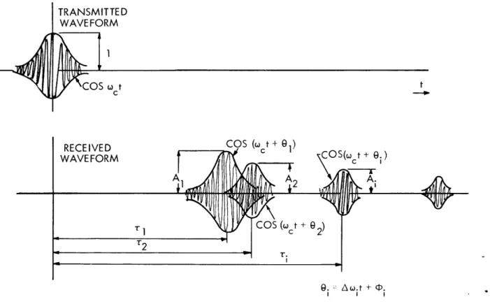
The model that we utilize is the same as the one used by Turin,21 except that we allow a frequency shift caused by Doppler shift or offset of the local oscillator in the receiver. TRANSMITTED WAVE FORM ,COS t C t 9. -- A.t + . I II
Fig. 14. Model of ionospheric scattering propagation.
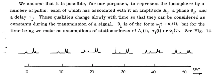
We assume that it is possible, for our purposes, to represent the ionosphere by a number of paths, each of which has associated with it an amplitude Ai, a phase Oi, and
a delay Ti. These qualities change slowly with time so that they can be considered as
constants during the transmission of a signal. 0i is of the form wit + i(t), but for the
time being we make no assumptions of stationariness of Ai(t), i(t) or i(t). See Fig. 14.
I I I I I I
0 10 20 30 40 50 SEC
Fig. 15. Impulse responses of ionospheric scattering taken 10 seconds apart.
The validity of this model can, of course, only be proved by comparing it with phys-ical data. The knowledge of HF ionospheric transmission that has been published is not too extensive, and the facts that support the model are, for the most part, of speculative
character. In Fig. 15 there are some pictures of the received signal over a 1685 -km ionospheric scattering link at 12. 35 mc when a short pulse (35 [isec) was transmitted. We see that the paths are well defined and their relative delay seems to stay constant, at least for times of the order of minutes. The response functions are taken from a note by Balser, Smith, and Warren.2
19
III. METHODS OF PREDICTION
3. 1 INTRODUCTION
According to our communication scheme the receiver measures the parameters of the channel model utilizing a sounding signal and then predicts the behavior of the chan-nel for the time interval used for message transmission. The fluctuations in the iono-sphere are random and, accordingly, the parameters in the model are determined by random processes. Thus, what we need is a prediction in a statistical sense, and we have the restriction that only a limited part of the past of the process is available. As we have pointed out, there is no evidence that the statistics of the ionosphere should be particularly simple, or even stationary. Our prediction operation should therefore not be sensitive to what kind of process it is applied to, and it is also desirable for it to be easily instrumented.
In the first part of this section some simple operations suitable for pure prediction are discussed and compared with optimum linear prediction. In the last part the prob-lem of prediction in the presence of noise is considered and some calculations are car-ried out on ionospheric data.
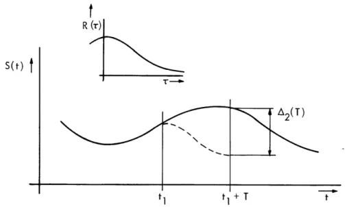
3.2 PURE PREDICTION a. Last-Value Prediction Perhaps the vicinity Fig. 16. In that kind of T is
the simplest prediction operation, when the function is known only in of a point, is to use the value at the point as a prediction. See the following discussion we use the term "last-value prediction" for operation. For a random process s(t) the error at prediction time
S(t)
t
tl tl+T t
Fig. 16. Last-value prediction.
20
p
A1(T) = s(tl+T) - s(tl), (33)
and the mean-square error is
E[ 12(T)] = E[s2(t 1+T)-2s(t1+T) s(t1)+s2(t1)] = 2[R(O)-R(T)],
where R(T) is the autocorrelation function (with the mean subtracted out) of s(t). If we define the correlation time T as
c R(Tc)= 2 R(O),
we see that
E[A2(T)] > R(O) for T > T
C
which means that the method is not suitable for T > Tc, since we then get a greater
mean-square error than the variance of the process itself. We notice that we do not use any statistical property of the process with this simple prediction.
b. Maximum Likelihood Prediction
If we know the second-order probability distribution for the process, we can use the value of s(tl+T) that maximizes p(s(tl+T)/s(tl)) as a prediction. We call this "maxi-mum likelihood" prediction and investigate the case of Gaussian statistics, in which the
second-order statistics are completely determined by the autocorrelation function. For a zero-mean Gaussian process, p(s(tl+T)/s(tl)) is a Gaussian distribution with
t
R (T I-S(t)t
T-. N1~~ tl A2(T) tl + T tFig. 17. Maximum likelihood prediction (Gaussian Case).
21
(34)
I
_ ._____
R(T) s(tl) R(T)
mean R( and variance R(O) l-R(0)J J. Since the Gaussian distribution is max-imum at the mean, this simply means we use the autocorrelation function as predictor (see Fig. 17). The mean-square error for prediction time T is
R(T) s(t1 2 R (T)
E[A2(T)] = E (t + T ) - R() = R(O) - (35)
We see that for small T the error is the same as for last-value prediction, but for large' T maximum likelihood prediction is better because E[A2(T)] can never exceed the vari-ance of the process.
For T = Tc, E[A2(TC)] = 3/4 R(O). We notice that for a first-order Markov process this kind of prediction is actually optimum. The reason for this is simply that the future behavior of the process is completely determined, in a statistical sense, by the last value.
c. Tangent Prediction
If we use the tangent of the curve as a predictor, we have another possible way of simple prediction, using only knowledge of the process around a single point.
Before we can discuss this type of prediction, we need to look into the question of derivatives of stochastic processes.
Derivatives of a Random Process
Consider a random process x(t) with variance ox and mean mx. Define a function
X(t+T) - x(t)
y(t, ) T T O. (36)
We have
E[y(t, T)] = 0
E[y(t, T)] = 1 E[x(t+T)-2(t)(t+T)+ (t)] = 2 [R(O)-R(T)].
T T
dx(t)
When T - O, y(t, T) is equal to dt , therefore the derivative has a finite variance only
if [R(O)-R(T)] goes to zero at least as fast as T . Since R(T) is an even function, either R'(0) = 0 or R'(+O) = -R'(-O).
In the last case the second derivative at zero does not exist, and differentiability of a random process is equivalent to requiring that R'(O) exists. We can state this in terms of the power density spectrum:
R"(O) = -42 f2 S(f) df. (37)
00
22
A sufficient and necessary condition for the derivative of a random process to exist (with probability one) is
Sr
J-00
f2S(f) df < oo.See Doob2 5 for a rigorous proof.
In the following we assume that the derivative of the random process exists and we thus have
E[(x'(t))2] = -R"(O) (38)
Finally we remark, that since the derivative is a linear function of the original process, the derivative of a Gaussian process has a Gaussian distribution with zero mean and var-iance R"(O).
As an example of processes which have no derivative, we can take the first order Markov process. It has an autocorrelation of the form
R(T) = R(O) eaITI (39)
(see Doob2 6 for a proof). This function has no second derivative at the origin and a sample function from the Markov process has no derivative (with probability one) at any point. This explains why the optimum linear predictor takes such a simple form as an exponential attenuator.
tl
A3(T)
tl+ T t
Fig. 18. Tangent prediction.
Tangent Prediction We obtain the error for prediction time T (see Fig. 18)
23
-l
___
_
I
A3(T) = s(t1+T) - [s(t1)+Ts'(t1)]. (40)
The mean-square error is
E[A2(T)] = E[s (tl+T)+s2 (t)+T2(s'(t)) 2 -2s(t1 +T)s(t )-2Ts(t+T)s(t1)+2Ts(t ) s(t)].
To evaluate this, we notice that
E[s(tl)s'(tl )]= lir E [(t 1) - lim R(T)-R(O)
T-) limi [R(T)-R(0)]
= R'(0) = 0
according to our assumption of differentiability. In the same way, E[s(t1+T) s'(t )] = -R(T)
and we have
2
E[A2(T)] = 2[R(O)-R(T)-- R"(O)+TR'(T)] = r(T). (41)
We call this the function for (T), and by comparing it with the error for last-value pre-diction we can write
r(T) = E[a2(T)] = E[A2(T)] - T[TR"(0)-2R'(T)]. (42)
As can be seen from Eq. 36, R"(0) is always negative; and for a monotonically decreasing autocorrelation R'(T) is negative for all T. In this case tangent prediction is better than the last-value prediction, at least for small values of T.
To get some insight into the expected performance of the different simple prediction schemes and to be able to compare them with optimum linear prediction, we work out a few examples, assuming certain forms of the autocorrelation function.
d. Examples
Example 2
Let us first compare the simple prediction methods for the autocorrelation of the form
R(T) = R(O) exp (T) (43)
In this case
E[A(T)]= 2R(O)[I -exp T (44)
E[A?2(T)] = R(O) r(T) = R(O)
L
1 - exp
2Tq2
TZI+
+2
)
exp
)
o \ ToI
(45) (46) T = T~linF~
C OThese functions are plotted in Fig. 19, and we see that as long as T < Tc the tangent
prediction gives the smallest error.
EACT)] Rs(O) 1 .0 0.5 0 EEA2(T)]/
1 ./
E [A2(T)] 2 T 2 T 0 0.5 1.0 -o ToFig. 19. Comparison between simple predictions (Example 2).
Example 3
To be able to compare with optimum linear prediction, consider a process with power density spectrum
,2
S2(f) =
(a2+f2)2
(47)
The corresponding autocorrelation is the Fourier transform of S(f). Applying residue calculus, we have k2 ej2rf7 R2(T) = 2rj Res (a2+f2)2 f=ja - .
~f=
ja (T > 0) which gives 25 __ __ R S(T) RSe(48)
2a
1 and T = 2
o 2-rra R2(T) is plotted in Fig. 20, from which we see that the
correlation time Tc is approximately 1. 7To .
To evaluate the error of the optimum predictor, we take the "realizable part" of S2(f).
G(f) = k (ja-f)2
and the corresponding function in the time domain is
g2(t) = k e ft dt = 00 (ja-f) k ej2Tft 2rrj Res ja-f -'ja-f) - f=ja (t>O) which gives = k47r2t e g2(t) A =0 t T0 t >_0 (49) t < 0.
The mean-square error for the optimum linear predictor for prediction time T is
E(T) = g(t) dt.
(See Davenport and Root2 7 for a derivation.) In our particular case we have
E2(T) = k2 16r4 t2 0 dt = cr2 -2 +2 T + 2 exp T T / (50) To get the error for the tangent predictor we obtain from Eq. 48
2 R2(0) = 2 T 0 T 2T TO R2(T) = -a2-2 e T
which by substitution in (41) yields
26 _ ___ R (T) = + - exp 2 2 T0 T0I exp T2t 0
R2(r) R(O) C _ = 1.7 (a) R3(r) R(O) t 1.0 0.5 0 c = 2.3 0 (b)
Fig. 20. Autocorrelation functions in Examples 3 and 4.
27 r T o - ---
~~~~~~_
_I__
I AS2(
/
)PTIMUM NEAR PREDICTION 0 0.5 'c 1.0 -2r TO 0 1TFig. 21. Tangent prediction compared with optimum prediction (Example 3).
r
(T)= 2+
2(1
+ T + )exp T . (51)O T
In Fig. 21, E2(T) and r 2(T) are plotted. We notice that when T << TO
E2(T) r2(T) 3 4 T2
The tangent prediction is thus "asymptotically optimum" in this special case. The reason is rather obvious. Since the fourth derivative of R2(T) does not exist at zero, the sample functions do not have a second derivative and it is not surprising that the optimum pre-diction is essentially linear extrapolation for small prepre-diction time.
A more complete discussion of optimum prediction for this particular correlation function has been given by Lee. 13
Example 4
Consider a random process in which the sample functions have derivatives of higher order than the first.
28 nmu)I £2 R(O) 0.4 0.3 0.2 0.1 A _ __ __ r'2 r S I I V
k2 S3(f) =
(a2+f2)3 In this case we have
2 k23w 8a5
ITI
+
---+
T o 3 1 and T = 1R3(T) is plotted in Fig. 20 which gives a correlation time Tc of approximately 2. 3To .
G3(f) = 3 (ja-f) t = k4r 3t2 e g3(t) ==0 t 0 (54) t<0
which gives the mean-square errors
E3(T) = 3 1- + 2 2 +- 3 3 0o T O T f T T0 L_~ +
~
+ 0 2 T3 T4 4 T e ] o · 2T 1 3 T0+ T -- T
eT iT~ e l ] .In Fig. 22, E3(T) and 3(T) are plotted. For small values of T we have
E3(T) = 5T3 T
T << T
0
In this case the tangent prediction gives a one order of magnitude larger error for small prediction time. According to Fig. 22 it is nevertheless performing rather well com-pared with optimum prediction as long as the prediction time is shorter than the
29 Take R3(T) = 3 (52) where (53) (55) (56)
-
I
---·---- · I
---1 2 4\ r (T) 4 a'37 0 oKkU) E3 R(O) 1 .0 0.5 0
Fig. 22. Tangent prediction compared with optimum prediction (Example 4). correlation time.
As long as we are working with power density spectra that are rational functions, the integral
&S o00fZn S(f) df
is not convergent for n larger than a certain value, and accordingly the sample functions cannot have derivatives of arbitrarily high order. The two examples that we have given seem to indicate that it should be possible to obtain a prediction that is "asymptotically optimum" (for T approaching zero) by using the existing terms in the Taylor series expansion of the sample function. If we apply this point of view, tangent prediction can be considered as the first-order approximation of such an "asymptotically optimum" pre-dictor.
e. Conclusions
It is difficult to make any general statements on the basis of a few examples, but the previous discussion supports the view that tangent prediction should not be an
30
__ I _________________I__·
r3 -1-1r
unreasonable thing to do, at least under certain circumstances. To be able to construct an optimum predictor, we need to know the power density spectrum, or autocorrelation function, of the process. The tangent prediction, on the other hand, does not use any statistical properties of the process and it is simple to instrument. Since obtaining the derivative is a linear process, tangent prediction is, of course, always inferior to opti-mum linear prediction. If, on the contrary, we do not know the autocorrelation function accurately enough, or use a predictor design for a particular prediction time under a maximum time interval, we could perhaps do just as well with the simpler tangent pre-diction. The mean-square error of the optimum predictor can never exceed the vari-ance of the process, but there is no limitation for the error of tangent prediction for large prediction time. If we want to employ tangent prediction, we must be sure that the prediction time is at least not greater than (say) the correlation time for the process.
Moreover, we have seen that it is mainly useful only for random processes with mono-tonically decreasing autocorrelation functions.
We shall now modify the prediction operation in order to work with processes that are disturbed by noise.
3.3 SMOOTHING AND PREDICTION
Noise is often present together with the random process that is to be predicted. Tan-gent prediction cannot be expected to perform well in that case. Assume that we have a signal s(t), together with noise n(t), so that the wave that we have to work on to predict s(t) is y(t) = s(t) + n(t). The derivative of y(t) is s'(t) + n'(t), and, even if n(t) is much smaller than s(t), its derivative n'(t) need not be small compared with s'(t).
To employ the idea of tangent prediction and to be able to introduce the necessary smoothing operation, we assume that the random process y(t) is sampled at times 6 seconds apart. If we use a certain number of samples to compute a regression line for use as a predictor, we have an operation that averages out the effects of the noise. In
y(t)
-T o T t
Fig. 23. Regression line prediction.
the noiseless case it is identical to tangent prediction when 6 becomes very small. See Fig. 23.
a. Regression-Line Prediction
Let us state the problem more precisely and derive an expression for the mean-square error. Assume that we have samples of a wide sense stationary random process y(t) = s(t) + n(t) sampled at times 6 seconds apart. To predict s(t) we use a straight line a + bt, where a and b are chosen so that
N
(a, b) = E [y(-v6)-(a-bv6)]2 (57)
v=O
is minimum. The expressions for a and b for the particular time origin chosen in Fig. 23 are given in Appendix C.
The mean-square error at prediction time T is
A(T) = E[(s(T)-(a+bT))2]. (58)
This expression is evaluated in Appendix C with the following assumptions: the noise has zero mean and is uncorrelated with the signal and is also uncorrelated between dif-ferent samples. It is assumed that the time T used to compute the regression line is
short compared with the correlation time for the signal. Under these assumptions, we have
A(T) = (T) + (T)
[+
N-i 2 nT +3 T 2N (59)Here, r(T) is the error for tangent prediction. @(T) = T (R0(T)-R(O))
N2 D(N) =
(N+1)(N+2)
T= N6
and a- = E[n (t)] is the variance of the noise.
n
Since we have the relation
R"(T) = 42 S4S(f ) f S df >-4w2$ fs(f) df = R(O),
we see that (T) 0, and regression-line prediction thus always gives a greater error than tangent prediction.
The second term in A(T) is increasing for increasing T and it is possible to
inter-pret it as being due to the fact that the regression time is equal to the derivative only
32
when T goes to zero. The third term depends on the noise. Since we have assumed
that the noise is uncorrelated between samples, it is natural to get the result that the term decreases as 1/N for large N. This means that it is advantageous to increase the sampling rate, at least as long as the noise is still uncorrelated between samples.
Contrary to other smoothing operations, any attempt to filter out the noise before regression-line prediction only gives greater error.
b. Minimization of the Mean-Square Error
The second term in A(T) is increasing and the third term is decreasing with T, and
for a given T and 6 it is possible to minimize A(T) by choosing T properly. Let us work this out for N >> 1. We can write
A(T) -r(T) + T (T) T + 6 T 2 + 3 + ] T T If we call T/T = a, we get A) (T) [
Li46+-.
aT T + 2 3 T a n4 = 3 = (a). (60) n a ' (T) T 2a2 + 6a + 9The function l(a) is plotted in Fig. 24. As an example, consider
Rs(t) = r exps 4)
with To = 20 sec; T = 10 sec; 6 = 0. 5 X 10- 3 sec (corresponding to wn 10 cps); and
2 0 n
()'s = 10 . We obtain 1{2(a) = 6.7 X 10 . According to Fig. 24 the corresponding 0. 03 X 10
a is approximately 0. 03 which gives N = = 600 and our assumption of N large
0.5 X 10 is satisfied.
If we are not willing to compute the regression line by using more than a certain num-ber of samples, we have another minimization problem. Given T and N, determine the
T N6
6 that minimizes A(T). Remembering that a = ave
a(T) T(T) N-1 4(N) 1 AdF =
~T
N 1+N-a - 6 1 +3 2 =0 6 = T N T 3 which gives 33 _ ___~~~~~~~~~~~~~~~~~~~~~~~~~~I.10- 6 10- 5 10- 2 Q1 10- 1
Fig. 24. The function l21(a).
N= 1
N= 100
10 110
Fig. 25. The function (N, a).
34 at 10 -10-8 I
I
a
10 10I-q
1 A 10- y 10- 4 '2 )o12 Na3 [+ N-l I]
n L3N . (N, a).(61)
(T) -(N)[2+a] 2(N, a).
f2 is plotted in Fig. 25 as a function of a for different values of N.
For the same example as before we get 22(N, a) = 0. 04, which for N = 10 gives a =
0. 15.
The practical value of these minimization procedures is limited by the fact that the derivation of A(T) was made with the assumption of T small.
3.4 COMPUTATIONS ON IONOSPHERIC DATA a. Source of Data
The data were obtained from Group 34 of Lincoln Laboratory, M. I. T. The trans-mission link used was 1566 km from Atlanta, Georgia, to Ipswich, Massachusetts. A pulse of approximately Gaussian shape and bandwidth 30 kcps was transmitted every
1/15 sec with a transmitter peak power of 10 kw. Through a gating circuit at the receiver the maximum amplitude of the received pulses corresponding to the different paths was
recorded. A "Datrac" equipment was used to quantize the samples into 64 levels and they were put onto magnetic tape as 6-bit numbers in a format corresponding to that for the IBM 709 computer. The records thus correspond to 6-bit samples of the path
strength sampled 15 times a second.
b. Presentation of the Data
From a large collection of data two records were chosen rather arbitrarily. These were obtained on February 16, 1960, at 10:52 a. m. and 12:12 p. m. EST, respectively, and the carrier frequencies used were 8. 35 mc and 18. 45 mc, respectively. Of the first record, which we call A, 9724 samples were available corresponding to a recording time of approximately 11 minutes. Record A is probably a return from the F-layer of the ionosphere making 3 hops. In Fig. 26 it is plotted from the magnetic tape by the use of the computer. In the figure is also the identification word on the tape. The second
recording, which we call B, contained 5271 samples, corresponding to approximately 6 minutes recording time. Record B is classified as a -hop F-layer return and it is plotted in Fig. 27.
Record A looks more stationary than record B and to show this the mean and var-iance, computed by using the first and second half of the record, are given below.
Record A Record B
Whole Whole
Part of record: 1 st half 2nd half Record 1st half 2nd half Record
Mean 18.32 21.47 19.89 31.11 39.99 35.55
Variance 79.0 107.3 95.6 146. 1 263.5 224.5
) n $4 0 O o O0 O I o 2 0 a -bD I 1 C Z Z C tL~ L D.C 0- (D O W v -CD I CD
36
C, LL I-2 I-D X) 14. to C'.' C 0 0I Lod
z LD C C a C L 0o o .-4 C, .-4 a) "4 k a) tC) I-: II z O rr wz
0 C0 w ir a.J E _ -- In .u f I I I Li wA . - ,
T
K ( R(O 0.5 0 0Fig. 28. Autocorrelation function, Record A.
R(r) I R(O) 1.0 0.5 0-.i t A | RECORD B | a = 224.5 r~ I I I I I I I I I '-0 10 20 30 40 50 60 70 80 90
Fig. 29. Autocorrelation function, Record B,
Examination of the distribution functions for the records shows that Record A is approx-imately Rayleigh distributed; Record B is neither Rayleigh nor Rician.
The normalized autocorrelation functions for the records are presented in Figs. 28 and 29.
c. Results
Regression-line prediction was performed on the two records with the use of a com-puter. The computer calculated a regression line, using a certain number of samples corresponding to the prediction time T, and determined a new regression line. The pre-diction error was defined as the difference between the end of the old regression line and the beginning of the new one. The procedure was repeated through the whole record. In Figs. 30 and 31 the variance of the prediction error is plotted versus prediction time.
37
____
N = 20
N= 10
RECORD A
N= 5
Fig. 30. Mean-square prediction error, Record A.
N=10
RECORD B
10
Fig. 31. Mean-square prediction error, Record B.
38 CURVE 10 1.0 A(T) 2 a 0.5 0 A(T) 2 a 0.5 0 a
D.
. __)o
8Different curves are given corresponding to number of samples used to compute the regression line. The statistics of the error were also computed and in Figs. 32 and 33 the distribution functions are given for different prediction times, plotted on normal distribution paper.
Record B is hardly stationary over the recording time. We can expect the prediction error to be more stationary than the process itself; and to illustrate this the prediction error is plotted below the corresponding record in Figs. 26 and 27.
To compare the calculated mean-square error with the theoretical formula (59) we need to know certain derivatives of the autocorrelation function and the signal-to-noise
7
t
4<_
T1-
1
IL
l l
.. , .
' ' I
I1 II
1 !
1- 1:.I
7
!
H~
·.
.
'I't'- it-I. -· i ' . 1: I -1-1 - i:
liii
1+ 4'1 I .... |1+H
:A1
-1,
:
1. . .i. 1 ''; -r--I L7t! .
I i
r , . ..
k
, : t: i I | , ; | ,-i' ' I , ,ii ! : :I ! _-e-... I . .: 1: - II
1 t I t*-,;li r --L-i _11hf.
4 .. - ! I 1 r: 5/1
I-'i l T:t: I ; -I i l I. . . i,! ...: 1 . I 1. .i
-:
I1
O 5 I'. .
-P'I
:
I II I II I% I I .s 1Fig. 32. Distribution functions for the error, Record A.
39