HAL Id: hal-01308801
https://hal.inria.fr/hal-01308801v3
Submitted on 22 Feb 2018
HAL is a multi-disciplinary open access
archive for the deposit and dissemination of
sci-entific research documents, whether they are
pub-lished or not. The documents may come from
teaching and research institutions in France or
abroad, or from public or private research centers.
L’archive ouverte pluridisciplinaire HAL, est
destinée au dépôt et à la diffusion de documents
scientifiques de niveau recherche, publiés ou non,
émanant des établissements d’enseignement et de
recherche français ou étrangers, des laboratoires
publics ou privés.
Finite Wordlength FIR Filters
Nicolas Brisebarre, Silviu-Ioan Filip, Guillaume Hanrot
To cite this version:
Nicolas Brisebarre, Silviu-Ioan Filip, Guillaume Hanrot. A Lattice Basis Reduction Approach for
the Design of Finite Wordlength FIR Filters. IEEE Transactions on Signal Processing, Institute
of Electrical and Electronics Engineers, 2018, 66 (10), pp.2673-2684. �10.1109/TSP.2018.2812739�.
�hal-01308801v3�
A Lattice Basis Reduction Approach for the Design
of Finite Wordlength FIR Filters
Nicolas Brisebarre, Silviu-Ioan Filip and Guillaume Hanrot
Abstract—Many applications of finite impulse response (FIR) digital filters impose strict format constraints for the filter coeffi-cients. Such requirements increase the complexity of determining optimal designs for the problem at hand. We introduce a fast and efficient method, based on the computation of good nodes for polynomial interpolation and Euclidean lattice basis reduction. Experiments show that it returns quasi-optimal finite wordlength FIR filters; compared to previous approaches it also scales remarkably well (length 125 filters are treated in < 9s). It also proves useful for accelerating the determination of optimal finite wordlength FIR filters.
Index Terms—BKZ algorithm, Euclidean Lattice, finite wordlength, FIR coefficient quantization, FIR digital filters, HKZ algorithm, lattice basis reduction, LLL algorithm, minimax approximation
I. INTRODUCTION
T
HE efficient design of FIR filters has been an active research topic in Digital Signal Processing (DSP) for several decades now. An important class of practical problems is related to the discrete nature of the representation space used for storing the filter coefficients (usually fixed-point or floating-point formats).Typical constraints are that these coefficients be representable as signed𝑏-bit integer values (up to a scaling factor) or that they have low complexity, such as them being sums of only a small number of power-of-two terms. While the first requirement is useful for implementation on fixed-point DSP processors, the second one occurs when one wants to construct multiplierless filtering circuits. It is addressed, for instance, in [1]–[11]. Our focus will be on the first requirement, in the case of direct-form FIR filters. This coefficient quantization issue has been considered as early as [12] (see also [13], the introduction of which gives an account on related work from the 1970s).
To better illustrate the problem, consider the following simple toy example. We use it for pedagogical purposes only, as in this case, an elementary analysis of the situation suffices to determine an optimal solution. We hope it allows the reader to quickly grasp the context of our study.
We want to compute a length 5 linear phase lowpass FIR filter with 5-bit wide fixed-point coefficients and uniformly
N. Brisebarre and G. Hanrot are with CNRS, ÉNS de Lyon, Inria, Université Claude Bernard Lyon 1, Laboratoire LIP (UMR 5668), 15 parvis René-Descartes, F-69007 Lyon, France.
E-mail: nicolas.brisebarre@ens-lyon.fr,guillaume.hanrot@ens-lyon.fr S-I. Filip is with CNRS, ÉNS de Lyon, Inria, Université Claude Bernard Lyon 1, Laboratoire LIP (UMR 5668), Lyon, France and Mathematical Institute, University of Oxford, Oxford, UK.
E-mail: silviu.filip@inria.fr
This work was partly supported by the FastRelax project of the French Agence Nationale de la Recherche.
weighted passband [0, 0.4𝜋] and stopband [0.5𝜋, 𝜋]. If we let 𝐷(𝜔) = 1 for 𝜔 ∈ [0, 0.4𝜋] and 𝐷(𝜔) = 0 if 𝜔 ∈ [0.5𝜋, 𝜋], we want 𝑎0, 𝑎1 and 𝑎2 ∈ {−24, . . . , 24 − 1} such that the approximation error max 𝜔∈[0,0.4𝜋]∪[0.5𝜋,𝜋] ⃒ ⃒ ⃒ 𝑎0 24 + 𝑎1 23cos(𝜔) + 𝑎2 23cos(2𝜔)− 𝐷(𝜔) ⃒ ⃒ ⃒ is as small as possible.
The Parks-McClellan algorithm [14], for instance, outputs an optimal infinite precision frequency response 𝐻*(𝜔) = 0.430· · ·+0.860 · · · cos(𝜔)+0.069 · · · cos(2𝜔) and correspond-ing approximation error 𝐸* = 0.360· · · . If we round each coefficient towards the nearest number of the form 𝑘/23 (or 𝑘/24 for the constant coefficient), we obtain 𝐻
naive(𝜔) = 7 24 + 7 23 cos(𝜔) + 1
23cos(2𝜔), and a corresponding error
𝐸naive= 0.4375. On the other hand, the approach we introduce in the subsequent sections returns𝐻(𝜔) = 8
24 +
6
23cos(𝜔) +
1
23cos(2𝜔), which improves the error to 𝐸 = 0.375. Using,
for instance, a mixed integer linear programming (MILP) routine, we obtain that𝐻 is actually an optimal 5-bit coefficient frequency response𝐻opt and𝐸 is the optimal approximation error𝐸opt.
This example displays two interesting facts:
∙ The straightforward approach, which we call “naive rounding”, consisting in rounding each coefficient of the infinite precision response to the nearest coefficient fitting the imposed constraints, may, even in very simple cases, yield results which are far from optimal (for instance, [15] mentions an example where a 30 dB improvement is observed).
∙ Another natural approach is to consider all the possible responses that we get by rounding up or down the coefficients of the infinite precision response. A first major drawback of this idea is that the number of possibilities is exponential in the degree of the filter. Moreover, our toy example shows that it is possible that none of them yields an optimal response, as was already noticed in [4]. In general, finding an optimal finite wordlength direct form FIR filter proves to be computationally expensive as the degree increases, with exact solvers making use of MILP techniques, sometimes combined with clever branch-and-bound strategies [1]–[3], [5], [13], [15]–[19]. To successfully cope with larger degrees, faster heuristics have also been proposed. They produce results that are, in many cases, quasi-optimal and can help speed up exact solvers. For instance, the approach introduced in [20], based on error spectrum shaping techniques, is routinely used inside MATLABTM for FIR coefficient
quantization. The methods developed in [4] (see also [21] for a variant) and [22] also produce very good results.
The rest of the paper introduces a novel and efficient method for designing quasi-optimal direct form FIR filters with fixed-point and/or floating-fixed-point coefficients. It is based on previous work for doing machine-efficient polynomial approximation of functions [23] combined with techniques that yield families of very good interpolation nodes [24]–[29]. As the filter degree gets higher, our approach improves significantly on the state of the art:
∙ As illustrated by Section VI, it returns results that are most of the time better than those computed by competing methods;
∙ When compared to exact MILP-based approaches (which are executed to completion or only for a limited time, depending on the degree), we often find the same result or a better one1: this happens for 8 out of the 15 examples discussed in Section VI-A;
∙ Further, our method is very robust and fast, especially when dealing with high degree designs.
Thanks to these features, we believe that it will prove very useful as a fast preliminary accelerator for exact solvers based on MILP. Finally, our tool is available as an open source C++ implementation2.
A. Sketch of our approach and outline of the paper
As we will show in SectionII, the problem that we address can be formulated as an MILP question, constructed from a sufficiently dense discretization of the target filter bands. The first key aspect of our work is the modeling of the MILP instance as a Closest Vector Problem (CVP), a fundamental question in the study of Euclidean lattices3 [30]. In particular, we take advantage of very efficient algorithms for computing approximate (and yet, at least in the filter design setting, often close to optimal) solutions to a CVP.
The CVP instance that we use is also constructed from a discretization of the filter frequency bands. For it to be effective, the following constraints are important:
∙ the number of discretization points should be as small as possible, both to produce a tractable CVP question and for a technical reason to be made clear in SectionV; ∙ the discretization points should be chosen so that the CVP
instance models as faithfully as possible the initial MILP problem.
As a second key idea, we propose several methods to compute such a discretization. These points are analogues to the so-called Chebyshev nodes on an interval and give rise to excellent polynomial approximations on the bands of the filter.
Then, we use an idea due to R. Kannan [31] to compute a good approximate solution to this CVP. A simple additional trick from [23] applied to this solution yields a certain frequency response 𝐻: in practice, its coefficients satisfy the requested
1in the time limited case.
2Seehttps://github.com/sfilip/fquantizer.
3Note that there is no link between Euclidean lattices and lattice wave
digital filters, as the one used in [7] for instance.
constraints and offer a very good approximation to the ideal frequency response.
After giving a precise statement of the problem that we want to solve in SectionII, Section IIIpresents the discretizations that we use, while SectionIVrecalls the algorithmic questions attached to Euclidean lattices that we face in our approach and some state-of-the art algorithms to address them. They are later used for detailing our method in SectionV. Examples and a comparison to other approaches are discussed in Section VI, followed by concluding remarks in SectionVII.
II. THE FINITE WORDLENGTH SETTING
We first recall some well-known ideas related to linear-phase FIR filter design [32]–[34]4. Such a process is typically carried out in the frequency domain. In case of an𝑁 -tap causal filter with real valued impulse response{ℎ[𝑛]}, the corresponding frequency response we want to optimize is
𝐻(𝜔) = 𝑁 −1 ∑︁ 𝑘=0 ℎ[𝑘]𝑒−𝑖𝜔𝑘 = 𝐺(𝜔)𝑒𝑖(𝐿𝜋 2 − 𝑁 −1 2 𝜔),
where𝐺 is a real valued function and 𝐿 is 0 or 1. Traditionally, there are four such types of FIR filters considered in practice, labeled from I through IV; they depend on the parity of the filter length𝑁 and on the symmetry of ℎ (positive for 𝐿 = 0 and negative for 𝐿 = 1). We can express 𝐺(𝜔) as 𝑄(𝜔)𝑃 (𝜔), where𝑃 (𝜔) is of the form:
𝑃 (𝜔) = 𝑛 ∑︁
𝑘=0
𝑝𝑘cos(𝑘𝜔).
Depending on the filter type,𝑄(𝜔) is either 1, cos(𝜔/2), sin(𝜔) or sin(𝜔/2). We have 𝑛 = ⌊𝑁/2⌋ and there are simple formulas linking theℎ[𝑘]’s and the 𝑝𝑘’s (see for instance [33, Ch. 15.8–15.10]).
Remark 1. If we consider the change of variable𝑥 = cos(𝜔), 𝑃 (𝜔) =∑︀𝑛
𝑘=0𝑝𝑘cos(𝑘𝜔) is in fact a polynomial of degree at most 𝑛 in cos(𝜔) expressed in the basis of Chebyshev polynomials(𝑇𝑘)06𝑘6𝑛 of the first kind,i.e.,
𝑃 (𝜔) = 𝑛 ∑︁ 𝑘=0 𝑝𝑘𝑇𝑘(cos(𝜔)) = 𝑛 ∑︁ 𝑘=0 𝑝𝑘𝑇𝑘(𝑥).
It will sometimes be convenient to see our problems in the language of polynomial approximation. When this is the case, 𝑥 will be the approximation variable and 𝑋 ⊆ [−1, 1] the transformed domain associated toΩ i.e., cos Ω.
While the focus of our presentation is on type I filters (hence 𝑄≡ 1), adapting it to the other three cases is straightforward. The optimal length 𝑁 frequency response with infinite precision coefficients is the solution of the following: Problem 1 (Equiripple (or minimax) FIR filter design). Let Ω be a compact subset of [0, 𝜋] and 𝐷(𝜔) an ideal frequency response, continuous onΩ. For a given filter degree 𝑛 ∈ N,
we want to determine 𝑃*(𝜔) = ∑︀𝑛 𝑘=0𝑝
*
𝑘cos(𝜔𝑘) such that the weighted error function𝐸*(𝜔) = 𝑊 (𝜔) (𝑃*(𝜔)
− 𝐷(𝜔)) hasminimum uniform norm
‖𝐸*
‖∞,Ω= sup 𝜔∈Ω|𝐸
*(𝜔) | ,
with the weight function𝑊 continuous and positive over Ω. There exists a unique solution to this problem [35, Ch. 3.4]: Theorem 1 (Alternation theorem). A necessary and sufficient condition for𝑃 (𝜔) to be the unique transfer function of degree at most 𝑛 that minimizes the weighted approximation error 𝛿Ω=‖𝐸(𝜔)‖∞,Ω is that 𝐸(𝜔) = 𝑊 (𝜔) (𝑃 (𝜔)− 𝐷(𝜔)) has at least𝑛 + 2 equioscillating extremal frequencies over Ω; i.e., there exist at least𝑛 + 2 values 𝜔𝑘 inΩ such that 𝜔0< 𝜔1< . . . < 𝜔𝑛+1 and
𝐸(𝜔𝑘) =−𝐸(𝜔𝑘+1) = 𝜆(−1)𝑘𝛿Ω, 𝑘 = 0, . . . , 𝑛, where 𝜆∈ {±1} is fixed.
The usual way to solve Problem 1 is to use, as already mentioned in Section I, the Parks-McClellan version of the Remez algorithm.
The finite wordlength version of Problem1that is of interest here, and also in practice, proves to be much harder to solve in general. For fixed-point coefficient quantization we can basically consider the impulse response coefficients to be scaled integers. If we want to use 𝑏-bit fixed-point values, we view them under the form 𝑚/𝑠, where 𝑚 is an integer in 𝐼𝑏 = {−2𝑏−1, . . . ,
−1, 0, 1, . . . , 2𝑏−1
− 1} and 𝑠 is a fixed scaling factor, which, in many cases, is a power of2. Let 𝜙0(𝜔) = 1/𝑠 and𝜙𝑘(𝜔) = 2 cos(𝑘𝜔)/𝑠 for 𝑘 = 1, . . . , 𝑛. We then have: Problem 2 (Finite wordlength minimax approximation). Con-sider Ω, 𝐷, 𝑛 and 𝑊 defined as in Problem 1. Determine 𝑃 (𝜔) = ∑︀𝑛
𝑘=0𝑚𝑘𝜙𝑘(𝜔), where 𝑚𝑘 ∈ 𝐼𝑏 for 𝑘 = 0, . . . , 𝑛, such that the error
sup
𝜔∈Ω|𝑊 (𝜔) (𝑃 (𝜔) − 𝐷(𝜔))|
(1) is minimal.
This problem always has a (not necessarily unique) solu-tion. Expressed as an optimization question, it becomes:
minimize 𝛿 subject to 𝑊 (𝜔) (︃ 𝑛 ∑︁ 𝑘=0 𝑚𝑘𝜙𝑘(𝜔)− 𝐷(𝜔) )︃ 6 𝛿, 𝜔∈ Ω, 𝑊 (𝜔) (︃ 𝐷(𝜔)− 𝑛 ∑︁ 𝑘=0 𝑚𝑘𝜙𝑘(𝜔) )︃ 6 𝛿, 𝜔∈ Ω, 𝑚𝑘∈ 𝐼𝑏, 𝑘 = 0, . . . , 𝑛. (2)
In practice,Ω is generally replaced with a finite discretization Ω𝑑, giving rise to a MILP instance. A number of points equal to16𝑛 usually suffices, according to [36].
The scaling factor𝑠, interpreted as the filter gain, can also be a design parameter. Optimizing for𝑠 as well can improve
the quality of the quantization error (1) by a small factor. The caveat is that finding the best𝑠 is nontrivial [15], [36], [37].
More general quantization problems where coefficients have different formats from one another (be it fixed-point of floating-point) can also be expressed using the framework of Problem2, with the difference being that each coefficient will have its own power of2 scaling factor 𝑠𝑘, 𝑘 = 0, . . . , 𝑛. Nevertheless, for simplicity, in the sequel we will only consider fixed-point quantization examples with a uniform scaling factor𝑠.
III. DISCRETIZATION OF THE PROBLEM
The first step of our approach is to discretize Problem 2
with (almost) as few points as possible, in order to speed up computation and also because our lattice-based approach requires a coarse discretization in order to return relevant results (we will make this point clear at the beginning of SectionV). We pickℓ points 𝜔0, . . . , 𝜔ℓ−1inΩ, with ℓ = 𝑛+1 or slightly larger than 𝑛 + 1, and we want to determine a 𝑃 (𝜔) = ∑︀𝑛
𝑘=0𝑚𝑘𝜙𝑘(𝜔), where 𝑚𝑘 ∈ 𝐼𝑏 for 𝑘 = 0, . . . , 𝑛, such that the error
max
𝑗=0,...,ℓ−1|𝑊 (𝜔𝑗) (𝑃 (𝜔𝑗)− 𝐷(𝜔𝑗))|
is as small as possible. A question immediately arises: how can we force this discretized version to be as faithful as possible to the initial Problem2?
Choosing appropriate points 𝜔𝑖 (or 𝑥𝑖= cos(𝜔𝑖)) is indeed critical for obtaining very good results [23]. We propose three complementary alternatives that work well together in our practical experimentations. The idea underlying the first two choices is to force the finite wordlength transfer function to mimic the minimax approximation𝑃*, whereas the third one corresponds to a relevant choice for the initialization of the Parks-McClellan algorithm to determine𝑃*.
A. Alternating extrema of the minimax error function Inspired by the characterization provided by Theorem1, the discretizationΩ𝑒we suggest is a set of 𝑛 + 2 frequencies that yield𝑛 + 2 alternating extrema for the error function 𝐸*.
There are some cases where the number of frequencies corresponding to these alternating extrema is larger than 𝑛 + 2. Therefore, we need an effective way to select exactly 𝑛 + 2 among them: the Parks-McClellan algorithm iteratively constructs such a list.
Remark 2. In practice, we use the implementation of the Parks-McClellan algorithm presented in [38] and available fromhttps:// github.com/ sfilip/ firpm: it computes𝑃* and a list of𝑛 + 2 nodes where 𝐸* equialternates, our Ω
𝑒.
B. “Zeros” of the minimax error function
This strategy is the analogue of one of the choices from [23]. And yet, there is a significant difference in our setting. Actually, in the case of a single interval [𝑎, 𝑏], Theorem 1 and the intermediate value theorem ensure that there exist, at least, 𝑛 + 1 points 𝑥0, . . . , 𝑥𝑛 in [𝑎, 𝑏] such that 𝐸*(𝑥𝑖) = 0 for 𝑖 = 0, . . . , 𝑛. Unfortunately, we do not have any such guarantee
in the present multi-interval setting: the number of zeros might be less than𝑛 + 1 so we complete the list by picking points that are half-way the endpoints of consecutive bands. Note that the latter points do not belong to Ω and we will explain in Section V(see discussion after Remark 7) how we use them. We execute the following:
Algorithm 1 “Zeros” of the minimax error discretization Input: the minimax approximation 𝑃*, ideal response 𝐷,
weight𝑊 , transformed domain 𝑋
Output: anℓ > 𝑛+1-element discretization Ω𝑧of[0, 𝜋] made of zeros of𝐸* and, if necessary, points that are half-way the extremities of the bands making up𝑋 = cos Ω // Take the zeros of 𝐸* over𝑋
1: 𝑋𝑧← roots(𝐸*, 𝑋)
// if the number of zeros is less than 𝑛 + 1, // take the midpoints of the transition bands // making up𝑋 (i.e., 𝑋 = ˙∪𝑘𝑗=1[𝑥 (𝑗) 0 , 𝑥 (𝑗) 1 ]) // with 𝑥(𝑗)1 < 𝑥 (𝑗+1) 0 for 𝑗 = 0, . . . , 𝑘− 1 2: 𝑗← 1 3: while|𝑋𝑧| < 𝑛 + 1 do 4: 𝑋𝑧← 𝑋𝑧∪ {︁ (𝑥(𝑗)1 + 𝑥 (𝑗+1) 0 )/2 }︁ 5: 𝑗← 𝑗 + 1 6: end while 7: Ω𝑧← arccos(𝑋𝑧)
Remark 3. One can prove that if a filter has𝑝 bands then the output discretization has at least𝑛+1 points and no more than 𝑛 + 𝑝− 1 points. In the practical cases presented in SectionVI, this discretization has exactly 𝑛 + 1 points (2 band case) or at most 𝑛 + 2 points (3 band case).
C. Approximate Fekete points
The second author has previously used this last approach as a numerically robust way of initializing the Parks-McClellan algorithm [38, Sec. 4.1–4.2]. We now briefly recall it.
For any compact set𝑋 ⊂ R, a set of Fekete points of degree 𝑛+2 are the elements of a set{𝑡0, . . . , 𝑡𝑛+1} ⊂ 𝑋 which max-imize the absolute value of the Vandermonde-like determinant |𝑤(𝑦𝑖)𝑇𝑗(𝑦𝑖)|06𝑖,𝑗6𝑛+1, with 𝑤(𝑥) = 𝑊 (arccos(𝑥)), where 𝑊 is the weight function used in the statements of Problems1
and 2 and the𝑇𝑗’s are the first 𝑛 + 2 Chebyshev polynomials of the first kind.
Unfortunately, computing them when𝑋 is not an interval is difficult in general. Still, approximate versions of such nodes, called Approximate Fekete Points (AFP), can be determined efficiently. The idea is to replace𝑋 by a suitable discretization 𝑌 ⊆ 𝑋 with 𝑚+1 > 𝑛+2 elements and extract Fekete points of 𝑌 . One good choice is that of so-called weakly admissible meshes [25]. The example we use consists of taking 𝑌 to be the union of the (𝑛 + 1)-th order Chebyshev nodes of second kind 𝜈𝑘 = 𝑎 + 𝑏 2 + 𝑏− 𝑎 2 cos (︂ 𝑘𝜋 𝑛 + 1 )︂ , 𝑘 = 0, . . . , 𝑛 + 1, scaled to each interval that makes up 𝑋. Even in this case, obtaining Fekete points over 𝑌 is an NP-hard problem [39].
We can, however, use an effective greedy algorithm based on column pivoting QR [24], [26]–[28]:
Algorithm 2 Approximate Fekete points discretization Input: discretized subset 𝑌 ={𝑦0, . . . , 𝑦𝑚} ⊆ 𝑋
Output: an 𝑛 + 2 distinct element set 𝑋afp ⊂ 𝑌 s.t. the Vandermonde-like submatrix V(𝑋afp) generated by the elements of𝑋afp has a large volume
// Initialization. V(𝑌 ) is the Vandermonde-like matrix //(𝑤(𝑦𝑖)𝑇𝑗(𝑦𝑖))06𝑖6𝑚,06𝑗6𝑛+1
1: A← V(𝑌 ), 𝑏 ∈ R𝑛+2, 𝑏← (1 · · · 1)𝑡 // QR-based Linear System Solver
2: using a column pivoting-based QR solver (via an equivalent of LAPACK’s DGEQP3 routine [40]), find w∈ R𝑚+1, a solution to the underdetermined system b= A𝑡w. // Subset Selection
3: take 𝑋afp as the set of elements from 𝑌 whose corre-sponding terms inside w are different from zero, that is, if 𝑦𝑖∈ 𝑌 and 𝑤𝑖̸= 0, then 𝑦𝑖∈ 𝑋afp.
Similar to the previous two choices, we will in fact work withΩafp= arccos(𝑋afp).
Remark 4. There are solid theoretical arguments for the AFP approach. They are based on the study of so-called Lebesgue constants and can be found in [38], [41].
Remark 5. Another alternative of good discretization grids is to take them according to the so-called equilibrium distribution for weighted minimax approximation on𝑋 [42]–[44]. We have not tested this idea here because it is more involved to set up than the approximate Fekete points method.
IV. THE CLOSEST VECTOR PROBLEM AND LATTICE BASIS REDUCTION
Let‖·‖2and‖·‖∞denote the usual Euclidean and supremum norms over Rℓ (i.e.,
‖v‖2 = (︁ ∑︀ℓ−1 𝑖=0𝑣 2 𝑖 )︁1/2 and ‖v‖∞ = maxℓ−1𝑖=0|𝑣𝑖|).
The Euclidean lattice structure is a fundamental component of various problems in Mathematics, Computer Science or Crystallography [30], [45]–[49]:
Definition 1. A lattice𝐿⊂ Rℓis the set of integer linear com-binations of a family(b1, . . . , b𝑑) of R-linearly independent vectors of Rℓ. We shall then say that(b𝑖)16𝑖6𝑑 is a basis of 𝐿, and that 𝑑(6 ℓ) is the dimension of 𝐿.
Finally, we define one of the most important algorithmic problems concerning Euclidean lattices:
Problem 3 (Closest vector problem (CVP)). Let || · || be a norm on Rℓ. Given as input a basis of a lattice 𝐿⊂ Rℓ of dimension𝑑, 𝑑 6 ℓ, and 𝑥∈ Rℓ, find 𝑦
∈ 𝐿 s.t. ||𝑥 − 𝑦|| = min{||𝑥 − 𝑣||, 𝑣 ∈ 𝐿}.
In order to find a good solution to Problem2, we address, after a suitable discretization, System (2). Up to a very mild relaxation of the constraint 𝑚𝑘∈ 𝐼𝑏 to𝑚𝑘∈ Z, the latter is actually a CVP in the supremum (or ‖ · ‖∞) norm. Although
CVP∞ can be attacked using MILP techniques, we propose to approximate it by the same CVP, but in the Euclidean (or‖ · ‖2) norm, a problem which we shall denote by CVP2. Even though, from a complexity-theoretic point of view, both problems are NP-hard, this change of perspective is motivated by the existence of a wealth of practical (i.e., efficient and with good performances) approximation algorithms to deal with this kind of problems.
The algorithms addressing a CVP2 usually rely on a preprocessing step called lattice basis reduction, a notion that we briefly discuss in SubsectionIV-A, together with three main tools for performing it: the LLL, BKZ and HKZ algorithms.
An idea due to Kannan [31], [50] will then allow us to use lattice basis reduction to obtain good approximate solutions of CVP2in the setting under study.
We also point out that the LLL algorithm has already been used in the digital filter design context, but in a different way [19]: in order to accelerate the MILP search for an optimal filter, Kodek determines, thanks to LLL5, a lower bound on the optimal approximation error, which is used as a first guess for 𝛿 in (2). Moreover, to the best of our knowledge, the present text discusses the first use of the BKZ, HKZ and Kannan embedding algorithms for a filter design purpose.
A. Lattice basis reduction
A lattice of dimension 𝑑 > 2 has infinitely many bases. Among those bases, the ones which are made up of short and somewhat orthogonal vectors are usually considered good, whereas the other ones are deemed bad. Lattice basis reduction algorithms allow one to move from a bad basis to a good one, an important preconditioning step in solving lattice problems. We shall consider three different lattice basis reduction algorithms, namely LLL, BKZ and HKZ. We shall not describe them nor their complete output – this is a rather technical topic and is out of the scope of this paper; we refer the reader to [30] for a detailed discussion of lattice basis reduction algorithms. Regarding their respective performances, the bottom line is that in terms of quality, LLL 6 BKZ 6 HKZ, while in terms of efficiency, unsurprisingly, LLL> BKZ > HKZ.
Remark 6. Actually, it seems that our input lattices and lattice bases are much better conditioned than expected, as all these algorithms seem to have a much better performance than expected on both quality and efficiency – HKZ-reducing a random lattice of dimension greater than 60 is, as of today, a considerable task, while we were able to do it on instances of degree 62 resulting from our problems in less than two minutes (see Section VI).
B. The CVP problem & Kannan’s embedding
When facing a CVP2 instance, one may choose to resort to exact, exponential-time approaches [51]. Even though they are efficient enough to deal with moderate size problems, we have found them to provide results which are not superior to
5Kodek actually applies LLL to a lattice which is dual to ours – which is
coherent with the use he makes of it.
our more efficient method. This might be explained by two reasons :
∙ as already observed, the lattice problems raised by digital filter design seem to be very well-conditioned, so that approximation algorithms tend to give much better results than expected (actually, often, optimal results).
∙ since CVP2 is already an approximate formulation of the problem to be solved, seeking an exact solution for it is not very meaningful. Actually, our main claim is that very good solutions to CVP2correspond to very good solutions to (2) (and SectionVIprovides evidence for that), whereas experience shows that optimal CVP2 solutions do not, in general, correspond to optimal solutions of (2).
We use Kannan’s embedding technique6[31] in the following way: given a basis(b1, . . . , b𝑑) of 𝐿 and the target vector t, we form the(𝑑 + 1)-dimensional lattice 𝐿′ of Rℓ+1 generated by the vectors b′𝑖:= (︂b𝑖 0 )︂ and t′:=(︂ t𝛾 )︂
, where𝛾 is a real pa-rameter to be chosen later on. If u is a short vector of the lattice 𝐿′, there exist 𝑢 1, . . . , 𝑢𝑑, 𝑢𝑑+1 such that u=∑︀ 𝑑 𝑘=1𝑢𝑘b′𝑘+ 𝑢𝑑+1t′; hence ‖u‖22= ⃦ ⃦ ⃦ ∑︀𝑑 𝑘=1𝑢𝑘b𝑘+ 𝑢𝑑+1t ⃦ ⃦ ⃦ 2 2+ 𝛾 2𝑢2 𝑑+1. If 𝛾 is taken large enough and u is short, we must have have𝑢𝑑+1=±1, meaning that ∓∑︀
𝑑
𝑘=1𝑢𝑘b𝑘∈ 𝐿 is close to the vector t. In practice, u is found as a vector of a reduced basis of𝐿′. The (heuristic) choice𝛾 = max𝑑
𝑘=1‖b𝑘‖2 always yielded a vector with𝑢𝑑+1=±1 in all experiments (see [41, Ch. 4.3.4] for a theoretical justification).
The entire procedure is summarized in Algorithm3. V. LATTICE-BASED FILTER DESIGN
We start by discretizing Problem 2: we pick ℓ(> 𝑛 + 1) points 𝜔0, . . . , 𝜔ℓ−1 in Ω and search for an approximation 𝑃 (𝜔) = ∑︀𝑛
𝑘=0𝑚𝑘𝜙𝑘(𝜔), where 𝑚𝑘 ∈ 𝐼𝑏 for 𝑘 = 0, . . . , 𝑛, such that the vectors
⎛ ⎜ ⎜ ⎜ ⎝ 𝑊 (𝜔0)∑︀ 𝑛 𝑘=0𝑚𝑘𝜙𝑘(𝜔0) 𝑊 (𝜔1)∑︀ 𝑛 𝑘=0𝑚𝑘𝜙𝑘(𝜔1) .. . 𝑊 (𝜔ℓ−1)∑︀𝑛𝑘=0𝑚𝑘𝜙𝑘(𝜔ℓ−1) ⎞ ⎟ ⎟ ⎟ ⎠ and ⎛ ⎜ ⎜ ⎜ ⎝ 𝑊 (𝜔0)𝐷(𝜔0) 𝑊 (𝜔1)𝐷(𝜔1) .. . 𝑊 (𝜔ℓ−1)𝐷(𝜔ℓ−1) ⎞ ⎟ ⎟ ⎟ ⎠
are as close as possible with respect to‖ · ‖∞. In other words, we need to find (𝑚0,· · · , 𝑚𝑛)∈ 𝐼𝑏𝑛+1 such that
𝑚0 ⎛ ⎜ ⎜ ⎜ ⎝ 𝑊 (𝜔0)𝜙0(𝜔0) 𝑊 (𝜔1)𝜙0(𝜔1) .. . 𝑊 (𝜔ℓ−1)𝜙0(𝜔ℓ−1) ⎞ ⎟ ⎟ ⎟ ⎠ ⏟ ⏞ b0 +· · ·+𝑚𝑛 ⎛ ⎜ ⎜ ⎜ ⎝ 𝑊 (𝜔0)𝜙𝑛(𝜔0) 𝑊 (𝜔1)𝜙𝑛(𝜔1) .. . 𝑊 (𝜔ℓ−1)𝜙𝑛(𝜔ℓ−1) ⎞ ⎟ ⎟ ⎟ ⎠ ⏟ ⏞ b𝑛 and t = (𝑊 (𝜔0)𝐷(𝜔0)· · · 𝑊 (𝜔ℓ−1)𝐷(𝜔ℓ−1)) 𝑡 are as close as possible to each other, i.e.,
minimize ‖𝑚0b0+ . . . + 𝑚𝑛b𝑛− t‖∞, (3) which is a CVP∞ instance, the Euclidean lattice under consideration being Zb0+ . . . + Zb𝑛⊂ Rℓ. We approximately
6Classically [31], [50], [52] Kannan’s idea is used in a much finer way, but
Algorithm 3 Kannan embedding
Input: basis(b1, . . . , b𝑑) of 𝐿⊂ Rℓ, target vector t∈ Rℓ, a lattice basis reduction algorithm (LLL, BKZ or HKZ) Output: m = (𝑚1· · · 𝑚𝑑)𝑡 ∈ Z𝑑 s.t. ∑︀
𝑑
𝑘=1𝑚𝑘b𝑘 ≈ t, change of basis matrix U∈ Z𝑑×𝑑
1: 𝛾← max16𝑘6𝑑‖b𝑘‖2
// Construct the embedded basis
2: B′←(︂b1 b2 · · · b𝑑 t
0 0 · · · 0 𝛾
)︂
// Perform basis reduction (LLL, BKZ or HKZ) on B′ // C′ =(︀𝑐′
𝑖,𝑗)︀ ∈ R(ℓ+1)×(𝑑+1)is the reduced basis // U′ =(︀𝑢′
𝑖,𝑗)︀ ∈ Z(𝑑+1)×(𝑑+1) is the change of basis // matrix (i.e., C′= B′U′)
3: (C′, U′)
← LatticeReduce(B′)
// Get change of basis matrix for B (i.e., first 𝑑 // rows and columns of U′)
4: U←(︀𝑢′ 𝑖,𝑗
)︀
16𝑖6𝑑,16𝑗6𝑑
// Extract element from last line and column of C′
5: 𝛾′ ← 𝑐′ℓ+1,𝑑+1
// Construct the outputs in terms of 𝛾′ and the last // column of U′ 6: 𝑠← 1 7: if𝛾′= −𝛾 then 8: 𝑠← −1 9: end if 10: for𝑖 = 1 to 𝑑 do 11: 𝑚𝑖← 𝑠 · 𝑢′𝑖,𝑑+1 12: end for
solve (3) in two steps, that we will present in more details in SubsectionV-A:
∙ the existence of well-tuned, practical approximation algo-rithms in the Euclidean setting leads us to (approximately) solve the ‖ · ‖2 version of (3) instead:
minimize ‖𝑚0b0+ . . . + 𝑚𝑛b𝑛− t‖2, (4) ∙ using combinations of the short vectors computed during the first step, we “turn” around the approximate solution of the CVP2instance (4) in order to improve the approximate solution of the CVP∞ instance (3). In fact, as the reader will see in V-A, we use this vicinity search to directly improve our solution to Problem2.
Note that working with (4) instead of directly solving (3) has the following important consequence. Since in Rℓ,
‖·‖∞6 ‖ · ‖2 6
√
ℓ‖ · ‖∞, we expect in general that small vectors with respect to the‖ · ‖2norm are also small when considering ‖ · ‖∞. Takingℓ close to the minimal value 𝑛 hence helps [23]. Remark 7. It also proves very useful to approximate 𝑃*, the minimax approximation, instead of𝐷: in this case, we consider t= (𝑊 (𝜔0)𝑃*(𝜔0)· · · 𝑊 (𝜔ℓ−1)𝑃*(𝜔ℓ−1))
𝑡
in(3) and (4). We have presented in SectionIIIthree families of discretiza-tion points:
∙ the alternating extrema of the minimax error function, cf. III-A, and approximate Fekete points, cf. III-C. We will use them to approximate both 𝐷 and 𝑃*;
∙ the “zeros” of the minimax error function, cf.III-B. Some of these points may belong to [0, 𝜋]∖ Ω, hence we can use this family only to approximate 𝑃*.
Eventually, we summarize our method in the form of a pseudo-code listing in SectionV-B.
A. Solving the CVP problem and a refinement trick
We saw in Section IV that (4) is an NP-hard problem, but argued that we can obtain an approximate solution quite efficiently by using a version of Kannan’s embedding technique. Applying Algorithm 3to (4) determines:
∙ a lattice vector∑︀𝑛
𝑘=0𝑚𝑘b𝑘 that is close to t with respect to‖ · ‖2 and hopefully close to t with respect to‖ · ‖∞, ∙ but also a reduced basis(c0, . . . , c𝑛) of (b0, . . . , b𝑛) (by applying the LLL, BKZ or HKZ algorithm and retrieving the change of basis matrix U).
Since the c𝑖 vectors are usually short with respect to the ‖ · ‖2 norm (and consequently with the‖ · ‖∞norm as well), we can use them to search in the vicinity of∑︀𝑛
𝑘=0𝑚𝑘b𝑘 with the goal of potentially improving the quality of our result with respect to Problem2.
In the function approximation setting, this idea is described in [53, p. 128]. Here, it translates to the following strategy: Algorithm 4 Vicinity search
Input: vector of discretized coefficients m ∈ Z𝑛+1, ideal response𝐷, weight 𝑊 , basis functions (𝜙𝑘)06𝑘6𝑛, change of basis matrix U∈ Z(𝑛+1)×(𝑛+1).
Output: vector of coefficients m′∈ Z𝑛+1. // Get initial approximation error & coefficients
1: 𝐸min← ‖𝑊 (𝜔) (∑︀ 𝑛
𝑘=0𝑚𝑘𝜙𝑘(𝜔)− 𝐷(𝜔))‖Ω,∞
2: m′← m
// Try to improve this initial approximation by selecting // two directions𝑑0 and𝑑1 in which to search
3: for𝑑0= 0 to 8 do
4: for𝑑1= 𝑑0+ 1 to 𝑛 do
5: u← U0:𝑛,𝑑0, v← U0:𝑛,𝑑1
// Update coefficients in these directions if it leads // to smaller approximation errors
6: for𝜀0, 𝜀1∈ {0, ±1} do 7: m′′← m 8: for𝑖 = 0 to 𝑛 do 9: 𝑚′′𝑖 ← 𝑚′′𝑖 + 𝑢𝑖𝜀0+ 𝑣𝑖𝜀1 10: end for 11: 𝐸← ‖𝑊 (𝜔) (∑︀𝑛𝑘=0𝑚′′𝑘𝜙𝑘(𝜔)− 𝐷(𝜔))‖Ω,∞ 12: if 𝐸 < 𝐸min then 13: 𝐸min← 𝐸 14: m′ ← m′′ 15: end if 16: end for 17: end for 18: end for
We limit the value of 𝑑0 to a small constant (here to eight) in order to keep the execution time reasonable (line 11 takes 𝑂(𝑛2) operations, and lines 3, 4 & 6 tell us that we execute it 𝑂(𝑛) times), but also because in practice we did not notice any significantly improved results by taking a larger search space. Increasing the number of search directions to three also helps, but we found the computational cost usually outweighs the improvements.
Remark 8. The lattice basis reduction approaches we use provide results that are hopefully close to the actual CVP solution, but they are not necessarily optimal. And yet, there are two quite encouraging points:
∙ the experiments in [41, §4.4.1] show that the output reduced basis is actually of excellent quality;
∙ the theoretical estimate in the same text [41, §4.4.3] supports our practical approach.
B. A pseudo-code synthesis of our approach
We can synthesize our whole approach as follows:
Algorithm 5 Lattice-based finite wordlength coefficient design Input: degree𝑛, ℓ-point discretization {𝜔0, . . . , 𝜔ℓ−1} of Ω (ℓ > 𝑛+1), scaling factor 𝑠, minimax response 𝑃*, weight 𝑊 , a lattice basis reduction algorithm LBR∈ {LLL, BKZ, HKZ}.
Output: fixed-point filter coefficientsℎ[𝑘], 𝑘 = 0, . . . , 2𝑛. // Construct the appropriate basis functions 𝜙0, . . . , 𝜙𝑛
1: 𝜙0(𝜔)← 1𝑠
2: for𝑘 = 1 to 𝑛 do
3: 𝜙𝑘(𝜔)←2 cos(𝑘𝜔)𝑠
4: end for
// Construct the lattice basis vectors
5: for𝑖 = 0 to 𝑛 do
6: b𝑖← (𝑊 (𝜔0)𝜙𝑖(𝜔0)· · · 𝑊 (𝜔ℓ−1)𝜙𝑖(𝜔ℓ−1))𝑡
7: end for
// Construct our two possible target vectors
8: t← (𝑊 (𝜔0)𝑃*(𝜔0)· · · 𝑊 (𝜔ℓ−1)𝑃*(𝜔ℓ−1))𝑡
9: t′← (𝑊 (𝜔0)𝐷(𝜔0)· · · 𝑊 (𝜔ℓ−1)𝐷(𝜔ℓ−1))𝑡
// Find approximate CVP solutions using Algorithm3
10: (m, U)← KannanEmbedding(B, t, LBR) 11: (m′, U′)← KannanEmbedding(B, t′, LBR)
// Use the vicinity search of Algorithm4 to improve the // quality of the solution
12: m← VicinitySearch(m, 𝐷, 𝑊, (𝜙𝑘)06𝑘6𝑛, U) 13: m′ ← VicinitySearch(m′, 𝐷, 𝑊, (𝜙𝑘)06𝑘6𝑛, U′) 14: 𝐸1← ‖𝑊 (𝜔) (∑︀ 𝑛 𝑘=0𝑚𝑘𝜙𝑘(𝜔)− 𝐷(𝜔))‖Ω,∞ 15: 𝐸2← ‖𝑊 (𝜔) (∑︀𝑛𝑘=0𝑚′𝑘𝜙𝑘(𝜔)− 𝐷(𝜔))‖Ω,∞ 16: if𝐸2< 𝐸1 then 17: m← m′ 18: end if
// Retrieve the corresponding finite wordlength coefficients
19: ℎ[𝑛]← 𝑚0 𝑠 20: for𝑘 = 0 to 𝑛− 1 do 21: ℎ[𝑘]← ℎ[2𝑛 − 𝑘] ← 𝑚𝑛−𝑘𝑠 22: end for TABLE I
FILTER SPECIFICATIONS CONSIDERED IN[22]. Filter Bands 𝐷(𝜔) 𝑊 (𝜔) A [0.5𝜋, 𝜋][0, 0.4𝜋] 10 11 B [0.5𝜋, 𝜋][0, 0.4𝜋] 10 101 C [0, 0.24𝜋] [0.4𝜋, 0.68𝜋] [0.84𝜋, 𝜋] 1 0 1 1 1 1 D [0, 0.24𝜋] [0.4𝜋, 0.68𝜋] [0.84𝜋, 𝜋] 1 0 1 1 10 1 E [0.02𝜋, 0.42𝜋] [0.52𝜋, 0.98𝜋] 1 0 1 1
Remark 9. Lines10 and11will generate the same reduced basis for B, so in practice we combine them to avoid any re-computations.
Remark 10. We call Algorithm 5 with the two discretiza-tion choices III-A and III-C. Regarding the discretization choice III-B, we call a reduced version of Algorithm 5: we don’t execute lines9,11,13and15that all deal with the ideal function𝐷. We keep the best result among the results returned from these calls.
VI. EXPERIMENTAL RESULTS
To illustrate the effectiveness of our method, we first compare it to the telescoping rounding approach introduced in [22], the error spectrum shaping method from [20] and the tree search approach of [4], based on least squares error optimization. To our knowledge, these7 are the most efficient quasi-optimal methods that explicitly treat the finite wordlength direct-form FIR design problem. We conclude this section with an account on the practical computation time of our code.
The following batch of tests were executed on an Intel i7-3687U CPU with a 64-bit Linux-based system and a g++ version 5.3.0 C++ compiler. As explained in Remark 9, all three discretization approaches presented in Section III are used, with the best result chosen in the end.
A. Kodek and Krisper’s telescoping rounding [22]
We start with the type I FIR filter specifications given in [22, Table 1], which we reproduce for convenience, in Table I. When referring to a particular design instance, we give the specification letter, filter length and scaling factor. For example, A35/8 denotes a design problem adhering to specification A, of length𝑁 = 35 (meaning a degree 𝑛 = 17 approximation), 𝑏 = 8 bits used to store the filter coefficients (sign bit included) and an𝑠 = 2𝑏−1scaling factor.
The results are highlighted in TableII:
∙ the first column lists the problem specification;
∙ the second one gives the minimax error 𝐸* computed using the Parks-McClellan algorithm.
All remaining columns represent approximation errors of the transfer function for various coefficient quantization strategies:
7Unfortunately, we were not able to make an accurate comparison with the
TABLE II
QUANTIZATION ERROR COMPARISON FOR THE FILTER SPECIFICATIONS GIVEN IN[22]. Filter Minimax
𝐸* Best known finitewordlength 𝐸 opt Naive rounding 𝐸naive Telescoping 𝐸tel LLL reduction 𝐸LLL BKZ reduction 𝐸BKZ HKZ reduction 𝐸HKZ A35/8 0.01595 0.02983 (M,L) 0.03266 0.03266 0.02983 0.02983 0.02983 A45/8 7.132 · 10−3 0.02962 (M,L) 0.03701 0.03186 0.02962 0.02962 0.02962 A125/21† 8.055 · 10−6 1.077 · 10−5(M) 1.620 · 10−5 1.179 · 10−5 1.161 · 10−5 1.168 · 10−5 1.251 · 10−5 B35/9 0.05275 0.07709 (M) 0.15879 0.07854 0.08205 0.08205 0.08205 B45/9 0.02111 0.05679 (M) 0.11719 0.06641 0.06041 0.06041 0.06041 B125/22† 2.499 · 10−5 2.959 · 10−5(M) 6.198 · 10−5 3.293 · 10−5 3.243 · 10−5 3.344 · 10−5 3.344 · 10−5 C35/8 2.631 · 10−3 0.01787 (M,T,L) 0.04687 0.01787 0.01787 0.01917 0.01917 C45/8 6.709 · 10−4 0.01609 (M,L) 0.03046 0.02103 0.01609 0.01609 0.02291 C125/21‡ 1.278 · 10−8 1.564 · 10−6(L) 8.203 · 10−6 2.1 · 10−6 1.606 · 10−6 1.564 · 10−6 1.564 · 10−6 D35/9 0.01044 0.03252 (M,L) 0.12189 0.03368 0.03252 0.03291 0.03291 D45/9 2.239 · 10−3 0.02612 (M) 0.10898 0.02859 0.02706 0.02805 0.02706 D125/22‡ 4.142 · 10−8 1.781 · 10−6(L) 3.425 · 10−5 2.16 · 10−6 1.864 · 10−6 1.781 · 10−6 1.826 · 10−6 E35/8 0.01761 0.03299 (M) 0.04692 0.03404 0.03349 0.03349 0.03349 E45/8 6.543 · 10−3 0.02887 (M,L) 0.03571 0.03403 0.03167 0.03094 0.02887 E125/21† 7.889 · 10−6 1.034 · 10−5(M) 1.479 · 10−5 1.127 · 10−5 1.215 · 10−5 1.245 · 10−5 1.162 · 10−5
∙ the third column presents optimal (or best known) finite wordlength errors𝐸opt: the errors for the length 125 filters are not proven to be optimal whereas the other ten errors are. Apart from the filters marked with the ‡, they are obtained using an MILP solver (with the values obtained in [22, Table 2]). In case of the problems marked with†, note that the exact solver was stopped after a certain time limit. We also indicate the methods attaining this optimal value, with M = (time-limited) MILP, L = lattice based (this paper), T = two coefficient telescoping rounding approach [22, Sec. 4].
∙ column four lists the errors obtained by simply rounding the real-valued minimax coefficients to their closest values in the imposed quantization format;
∙ the fifth column gives the best errors from using the two coefficient telescoping rounding approach of [22, Sec. 4]; ∙ the last three columns show the lattice-based quantization errors when choosing the LLL, BKZ and HKZ basis reduction option, respectively, when applying Algorithm5. A default block size of 8 was used when calling BKZ. For the last four columns, values reported in bold are the best out of the telescoping rounding approach and our approach.
We notice that lattice-based quantization gives results which are optimal (or the best known ones) in eight cases out of fifteen and the other seven cases are very close to the optimal ones. It outperforms telescoping rounding in twelve cases out of fifteen and yields the same (optimal) result in a thirteenth case: the use of the LLL option gives a better result in twelve cases and an identical (optimal) result in a thirteenth case, the use of the BKZ option gives a better result in eleven cases and the use of the HKZ option in nine cases. We remark, in particular, the good behavior of the LLL algorithm in all 15 test cases, further emphasizing the idea that the lattice bases we use are close to being reduced. Our approach seems to work particularly well when the gap between the minimax error and the naive rounding error is significant, which is the case where one is most interested in improvements over the naive rounding filter. Eventually, note that, in the C125/21 and D125/22 cases, our approach returns (in less than 8 seconds, see Subsection VI-D) results that are better than the ones provided by (time-limited) MILP tools.
B. Nielsen’s error spectrum shaping approach [20]
Consider now the finite wordlength low-pass filter specifica-tion [20, Sec. V] with passband[0, 0.4𝜋], stopband [0.6𝜋, 𝜋], stopband attenuation6−90 dB and passband peak to peak ripple6 0.01994 dB (passband attenuation −58.8 dB). The corresponding weighting function is
𝑊 (𝜔) = {︃
1, 𝜔∈ [0, 0.4𝜋], 1090−58.820 , 𝜔∈ [0.6𝜋, 𝜋].
The error spectrum shaping approach introduced in [20] and used by MATLABTM’s fixed-point filter design tools takes such a specification and produces quasi-optimal fixed-point coefficient filters that satisfy it. For instance, the constraincoeffwl function takes the magnitude bounds and a maximum coefficient wordlength as inputs. It produces an FIR filter with a coefficient format upper bounded by the maximal parameter value. The length of the filter is also taken to be as small as possible.
For coefficients stored on at most 15 bits, we can call
d = fdesign.lowpass(’Fp,Fst,Ap,Ast’,.4,.6,.01994,90); Hd = design(d,’equiripple’);
Hq = constraincoeffwl(Hd,15,’NoiseShaping’,true);
Running this stochastic routine 10 times, the best result we obtained had 𝑁 = 51, 15-bit coefficients, −95.17 dB attenuation and a0.0148 dB ripple. Our lattice based approach with the BKZ option was able to decrease the length to𝑁 = 47, 15-bit coefficients,−90.66 dB attenuation and 0.0192 dB ripple. See Figure1 for its magnitude response and TableIIIfor the coefficients.
C. Lim and Parker’s LMS criterion-based tree search ap-proach [4]
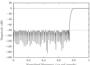
Similarly, we can take the high-pass specification from Example 1 in [4] consisting of a[0, 0.74𝜋] stopband, [0.8𝜋, 𝜋] passband, 17 bit wordlength (including sign bit) coefficients, stopband attenuation6−80 dB and passband peak to peak ripple6 0.1 dB (passband attenuation−44.79 dB). The result
−180 −160 −140 −120 −100 −80 −60 −40 −20 0 20 0 0.2 0.4 0.6 0.8 1 Magnitude (dB)
Normalized Frequency (×π rad/sample)
Fig. 1. The magnitude response of the finite wordlength filter produced by our lattice-based code on the example from SectionVI-B.
TABLE III
IMPULSE RESPONSE FOR THE DISCRETE COEFFICIENT FILTER MEETING THE SPECIFICATIONS OF[20, SEC. 5]
ℎ[𝑛] = ℎ[46 − 𝑛]FOR23 6 𝑛 6 46. Lowpass filter, 𝑁 = 47
Passband peak to peak ripple = 0.0192 dB Peak stopband attenuation = −90.66 dB Impulse response ×215 ℎ[23] = 15864 ℎ[15] = −358 ℎ[7] = −96 ℎ[22] = 10356 ℎ[14] = 628 ℎ[6] = 44 ℎ[21] = 508 ℎ[13] = 284 ℎ[5] = 56 ℎ[20] = −3260 ℎ[12] = −372 ℎ[4] = −14 ℎ[19] = −476 ℎ[11] = −216 ℎ[3] = −30 ℎ[18] = 1738 ℎ[10] = 204 ℎ[2] = −2 ℎ[17] = 420 ℎ[9] = 150 ℎ[1] = 10 ℎ[16] = −1040 ℎ[8] = −102 ℎ[0] = 4
they obtain has degree 𝑛 = 60, passband ripple 0.08 dB and stopband attenuation−80.3 dB, leading to the weight function
𝑊 (𝜔) = {︃
1080−44.7920 , 𝜔∈ [0, 0.74𝜋],
1, 𝜔∈ [0.8𝜋, 𝜋].
By using LLL as the basis reduction algorithm, we obtain a similar filter of degree 𝑛 = 60, with passband ripple 0.091 dB and stopband attenuation −80.03 dB in under 9 seconds; the resulting magnitude response is given in Figure 2, with coefficients in Table IV.
D. Computation time in practice
Analyzing the runtime of Algorithm 5 is dependent on the basis reduction approach used for the Kannan embedding portion of the computation (lines 10 and 11) and the short vector-based vicinity search (lines 12 and 13), which takes 𝑂(𝑛3). Actually, the lattice bases that appear in our problems are usually quite close to being reduced, making the Kannan embedding portion of the code much faster than the vicinity search (at least when using LLL and BKZ reductions). This can be seen for instance in TableV, which breaks down the execution time of our code, applied to the three discretizations mentioned in Section III, on the examples of TableII:
−180 −160 −140 −120 −100 −80 −60 −40 −20 0 20 0 0.2 0.4 0.6 0.8 1 Magnitude (dB)
Normalized Frequency (×π rad/sample)
Fig. 2. The magnitude response of the finite wordlength filter produced by our lattice-based code on the example from SectionVI-C.
TABLE IV
IMPULSE RESPONSE FOR THE DISCRETE COEFFICIENT FILTER MEETING THE SPECIFICATIONS OF[3, EXAMPLE1]
ℎ[𝑛] = ℎ[120 − 𝑛]FOR61 6 𝑛 6 120. Highpass filter, 𝑁 = 121
Passband peak to peak ripple = 0.091 dB Peak stopband attenuation = −80.03 dB Impulse response ×216 ℎ[60] = 14705 ℎ[39] = −593 ℎ[18] = −139 ℎ[59] = −13508 ℎ[38] = 148 ℎ[17] = 131 ℎ[58] = 10268 ℎ[37] = 301 ℎ[16] = −71 ℎ[57] = −5914 ℎ[36] = −555 ℎ[15] = −6 ℎ[56] = 1631 ℎ[35] = 529 ℎ[14] = 64 ℎ[55] = 1536 ℎ[34] = −274 ℎ[13] = −81 ℎ[54] = −3010 ℎ[33] = −65 ℎ[12] = 57 ℎ[53] = 2817 ℎ[32] = 325 ℎ[11] = −9 ℎ[52] = −1502 ℎ[31] = −402 ℎ[10] = −39 ℎ[51] = −135 ℎ[30] = 287 ℎ[9] = 67 ℎ[50] = 1358 ℎ[29] = −58 ℎ[8] = −68 ℎ[49] = −1749 ℎ[28] = −167 ℎ[7] = 46 ℎ[48] = 1308 ℎ[27] = 289 ℎ[6] = −14 ℎ[47] = −377 ℎ[26] = −269 ℎ[5] = −15 ℎ[46] = −559 ℎ[25] = 136 ℎ[4] = 32 ℎ[45] = 1095 ℎ[24] = 35 ℎ[3] = −35 ℎ[44] = −1063 ℎ[23] = −163 ℎ[2] = 28 ℎ[43] = 566 ℎ[22] = 199 ℎ[1] = −17 ℎ[42] = 107 ℎ[21] = −141 ℎ[0] = 8 ℎ[41] = −634 ℎ[20] = 29 ℎ[40] = 804 ℎ[19] = 80
∙ the first column lists the problem specification;
∙ the second one is the time required for finding the three discretizations;
∙ the following three columns show the computation time of the Euclidean lattice part of the code (lattice basis reduction and approximate CVP solving, which correspond to lines10 and 11 in Algorithm 5) when choosing the LLL, BKZ and HKZ basis reduction option, respectively; ∙ column six presents the vicinity search computation time,
which correspond to lines 12and13in Algorithm 5; ∙ the last column gives the total execution time of our code
when choosing the LLL option. The remaining steps are executed fast enough so that the values in this column are just slightly larger than the sum of the values presented
TABLE V
TIMINGS(IN SECONDS)WHEN USING THE THREE DISCRETIZATIONS OF
SECTIONIII. THE LAST COLUMN GIVES THE TOTAL RUNTIME WHENLLL
IS CHOSEN AS THE LATTICE BASIS REDUCTION ALGORITHM. Filter generationPoint LLL BKZ HKZ Vicinitysearch (LLL)Total A35/8 0.048 0.026 0.028 0.028 0.231 0.325 A45/8 0.047 0.033 0.035 0.035 0.474 0.571 A125/21 0.112 0.291 0.348 0.471 7.686 8.185 B35/9 0.112 0.018 0.019 0.027 0.243 0.401 B45/9 0.102 0.033 0.035 0.045 0.468 0.676 B125/22 0.191 0.296 0.342 1.194 7.746 8.314 C35/8 0.094 0.022 0.021 0.021 0.225 0.396 C45/8 0.107 0.032 0.036 0.037 0.414 0.611 C125/21 0.319 0.455 0.671 303.98 6.366 7.278 D35/9 0.162 0.019 0.021 0.021 0.211 0.411 D45/9 0.096 0.031 0.037 0.037 0.411 0.595 D125/22 0.251 0.435 0.784 335.38 6.240 7.042 E35/8 0.063 0.017 0.018 0.021 0.211 0.301 E45/8 0.089 0.018 0.031 0.031 0.420 0.574 E125/21 0.236 0.261 0.312 1.935 1.184 7.712 TABLE VI
HIGH DEGREE TYPEI FIRSPECIFICATIONS
Filter Bands 𝐷(𝜔) 𝑊 (𝜔) F [0, 0.2𝜋][0.205𝜋, 𝜋] 01 101 G [0, 0.4𝜋] [0.405𝜋, 0.7𝜋] [0.705𝜋, 𝜋] 1 0 1 1 10 1 H [0, 0.45𝜋] [0.47𝜋, 𝜋] 0 1 10 1 in columns 2, 3 and 6.
We used the fplll C++ library implementations [54] of the LLL, BKZ and HKZ algorithms.
One can note that our approach, when choosing the LLL option, is fast: for instance, it takes at most 8 seconds to compute a very good frequency response for the filters of length 125. Interestingly enough, the use of the BKZ option, which computes better reduced bases, leads to a very small computing time penalty. The use of the BKZ option allows us to compute the best, as of today, frequency responses for C125 and D125 in less than 8 seconds. Another remarkable fact is the excellent behavior of our approach when choosing the HKZ option: it is very fast in the cases of A125, B125 and E125 and offers a reasonable execution time in the cases of C125, D125 whereas the corresponding lattices have a dimension equal to, at least, 63, a size which usually means a very difficult challenge for an HKZ reduction attempt. In addition to the output quality, the efficiency of our approach strongly advocates for its use as a first accelerating step for exact MILP based approaches (where it would cause almost no time penalty).
TABLE VII
HIGH DEGREE QUANTIZATION RESULTS
Filter Minimax𝐸⋆ Naive rounding𝐸 naive LLL reduction 𝐸LLL Runtime in sec. F1601/18 8.64 · 10−4 3.41 · 10−3 1.20 · 10−3 846.85 G1201/16 4.78 · 10−3 1.21 · 10−2 5.79 · 10−3 567.01 H501/16 1.67 · 10−4 5.79 · 10−3 1.44 · 10−3 379.11
Remark 11. To further illustrate its robustness, let’s mention that our Euclidean lattice-based routine scales well to much larger degrees, as illustrated in TableVII, which adhere to the specifications from TableVI. The scaling factor used is again 𝑠 = 2𝑏−1. Note that:
∙ since the exhaustive enumeration performed by the vicinity search would be quite costly on such examples, we use a simple stochastic approach: take uniform random values of𝑑0, 𝑑1, 𝜀0, 𝜀1inside Algorithm4for one minute, keeping the best result at the end;
∙ if the filter degree is too large, at some point the leading coefficients of the optimal quantization will become zero [55]. We have avoided this scenario by considering only very narrow transition bands, which correspond to a slow decrease in the size of the minimax filter coefficients.
VII. CONCLUSION
We have developed a novel approach for designing machine-number coefficient FIR filters based on an idea previously introduced in [23], which transforms the design problem using the language of Euclidean lattices. The values obtained show that the method is extremely robust and competitive in practice. It frequently produces results which are close to optimal and/or beats other heuristic approaches.
There are several directions of research we are currently pursuing. The first is integrating this method into an FIR filter design suite for FPGA targets. The text [56] is a first attempt in this direction. IIR filter quantization using Euclidean lattices is another idea. There are several difficulties which have to be overcome in the rational IIR setting:
∙ nonlinearity of the transfer function;
∙ the approximation domain switches from Ω to a subset of the unit circle;
∙ ensuring stability of the transfer function (control the position of poles).
REFERENCES
[1] Y. C. Lim and A. Constantinides, “New integer programming scheme for nonrecursive digital filter design,” Electron. Lett., vol. 15, no. 25, pp. 812–813, Dec. 1979.
[2] Y. C. Lim, S. Parker, and A. Constantinides, “Finite Word Length FIR Filter Design using Integer Programming Over a Discrete Coefficient Space,” IEEE Trans. Acoust., Speech, Signal Process., vol. 30, no. 4, pp. 661–664, Aug. 1982.
[3] Y. C. Lim and S. Parker, “FIR Filter Design Over a Discrete Powers-of-Two Coefficient Space,” IEEE Trans. Acoust., Speech, Signal Process., vol. 31, no. 3, pp. 583–591, Jun. 1983.
[4] ——, “Discrete Coefficient FIR Digital Filter Design Based Upon an LMS Criteria,” IEEE Trans. Circuits Syst., vol. 30, no. 10, pp. 723–739, Oct. 1983.
[5] Y. C. Lim, R. Yang, D. Li, and J. Song, “Signed Power-of-Two Term Allocation Scheme for the Design of Digital Filters,” IEEE Trans. Circuits Syst. II, vol. 46, no. 5, pp. 577–584, May 1999.
[6] J. Yli-Kaakinen and T. Saramäki, “A systematic algorithm for the design of multiplierless FIR filters,” in The 2001 IEEE International Symposium on Circuits and Systems, 2001. ISCAS 2001. Sydney, Australia, May 6–9, vol. 2. IEEE, 2001, pp. 185–188.
[7] ——, “A Systematic Algorithm for the Design of Lattice Wave Digital Filters With Short-Coefficient Wordlength,” IEEE Trans. Circuits Syst., vol. 54, no. 8, pp. 1838–1851, Aug. 2007.
[8] J. Skaf and S. P. Boyd, “Filter Design With Low Complexity Coefficients,” IEEE Trans. Signal Process., vol. 56, no. 7, pp. 3162–3169, Jul. 2008.
[9] Y. Cao, K. Wang, W. Pei, Y. Liu, and Y. Zhang, “Design of High-Order Extrapolated Impulse Response FIR Filters with Signed Powers-of-Two Coefficients,” Circuits Syst. Signal Process., vol. 30, no. 5, pp. 963–985, 2011.
[10] D. Wei, “Design of discrete-time filters for efficient implementation,” Ph.D. dissertation, Massachusetts Institute of Technology, 2011. [Online]. Available:https://dspace.mit.edu/handle/1721.1/66470
[11] E. A. da Silva, L. Lovisolo, A. J. Dutra, and P. S. Diniz, “FIR Filter Design Based on Successive Approximation of Vectors,” IEEE Trans. Signal Process., vol. 62, no. 15, pp. 3833–3848, 2014.
[12] J. Knowles and E. Olcayto, “Coefficient Accuracy and Digital Filter Response,” IEEE Trans. Circuit Theory, vol. 15, no. 1, pp. 31–41, 1968. [13] D. M. Kodek, “Design of Optimal Finite Wordlength FIR Digital Filters Using Integer Programming Techniques,” IEEE Trans. Acoust., Speech, Signal Process., vol. 28, no. 3, pp. 304–308, Jun. 1980.
[14] T. W. Parks and J. H. McClellan, “Chebyshev Approximation for Nonrecursive Digital Filters with Linear Phase,” IEEE Trans. Circuit Theory, vol. 19, no. 2, pp. 189–194, March 1972.
[15] D. M. Kodek, “Performance limit of finite wordlength FIR digital filters,” IEEE Trans. Signal Process., vol. 53, no. 7, pp. 2462–2469, Jul. 2005. [16] D. M. Kodek and K. Steiglitz, “Comparison of Optimal and Local Search Methods for Designing Finite Wordlength FIR Digital Filters,” IEEE Trans. Circuits Syst., vol. 28, no. 1, pp. 28–32, 1981.
[17] O. Gustafsson and L. Wanhammar, “Design of linear-phase FIR filters combining subexpression sharing with MILP,” in The 2002 45th Midwest Symposium on Circuits and Systems, 2002. MWSCAS-2002., vol. 3, Aug. 2002, pp. 9–12.
[18] D. Shi and Y. J. Yu, “Design of Linear Phase FIR Filters With High Probability of Achieving Minimum Number of Adders,” IEEE Trans. Circuits Syst. I, vol. 58, no. 1, pp. 126–136, Jan. 2011.
[19] D. M. Kodek, “LLL Algorithm and the Optimal Finite Wordlength FIR Design,” IEEE Trans. Signal Process., vol. 60, no. 3, pp. 1493–1498, Mar. 2012.
[20] J. Nielsen, “Design of Linear-Phase Direct-Form FIR Digital Filters with Quantized Coefficients Using Error Spectrum Shaping,” IEEE Trans. Acoust., Speech, Signal Process., vol. 37, no. 7, pp. 1020–1026, Jul. 1989.
[21] G. Evangelista, “Design of optimum high-order finite-wordlength digital FIR filters with linear phase,” Signal Process., vol. 82, no. 2, pp. 187–194, 2002.
[22] D. M. Kodek and M. Krisper, “Telescoping rounding for suboptimal finite wordlength FIR digital filter design,” Digit. Signal Process., vol. 15, no. 6, pp. 522–535, 2005.
[23] N. Brisebarre and S. Chevillard, “Efficient polynomial 𝐿∞
-approximations,” in 18th IEEE Symposium on Computer Arithmetic, 2007. ARITH ’07, Jun. 2007, pp. 169–176.
[24] L. P. Bos and N. Levenberg, “On the calculation of approximate Fekete points: the univariate case,” Electron. Trans. Numer. Anal., vol. 30, pp. 377–397, 2008.
[25] J.-P. Calvi and N. Levenberg, “Uniform approximation by discrete least squares polynomials,” J. Approx. Theory, vol. 152, no. 1, pp. 82–100, May 2008.
[26] A. Sommariva and M. Vianello, “Computing approximate Fekete points by QR factorizations of Vandermonde matrices,” Comput. Math. Appl., vol. 57, no. 8, pp. 1324–1336, Apr. 2009.
[27] ——, “Approximate Fekete points for weighted polynomial interpolation,” Electron. Trans. Numer. Anal., vol. 37, pp. 1–22, 2010.
[28] L. P. Bos, J.-P. Calvi, N. Levenberg, A. Sommariva, and M. Vianello, “Geometric weakly admissible meshes, discrete least squares approxima-tions and approximate Fekete points,” Math. Comp, vol. 80, no. 275, pp. 1623–1638, 2011.
[29] S. De Marchi, F. Piazzon, A. Sommariva, and M. Vianello, “Polynomial Meshes: Computation and Approximation,” in Proceedings of the 15th International Conference on Computational and Mathematical Methods in Science and Engineering, 2015, pp. 414–425.
[30] P. Q. Nguyen and B. Vallée, Eds., The LLL Algorithm - Survey and Applications, ser. Information Security and Cryptography. Springer, 2010.
[31] R. Kannan, “Minkowski’s convex body theorem and integer program-ming,” Math. Oper. Res., vol. 12, no. 3, pp. 415–440, Aug. 1987. [32] A. V. Oppenheim and R. W. Schafer, Discrete-Time Signal Processing,
ser. Prentice-Hall Signal Processing Series. Prentice Hall, 2010. [33] A. Antoniou, Digital Signal Processing: Signals, Systems, and Filters.
McGraw-Hill Education, 2005.
[34] P. Prandoni and M. Vetterli, Signal Processing for Communications. Taylor & Francis, 2008. [Online]. Available:http://www.sp4comm.org/
[35] E. W. Cheney, Introduction to Approximation Theory, ser. AMS Chelsea Publishing Series. AMS Chelsea Pub., 1982.
[36] D. M. Kodek, “Design of optimal finite wordlength FIR digital filters,” in Proc. of the European Conference on Circuit Theory and Design, ECCTD ’99., vol. 1, Aug. 1999, pp. 401–404.
[37] Y. Lim, “Design of Discrete-Coefficient-Value Linear Phase FIR Filters with Optimum Normalized Peak Ripple Magnitude,” IEEE Trans. Circuits Syst., vol. 37, no. 12, pp. 1480–1486, Dec. 1990.
[38] S.-I. Filip, “A robust and scalable implementation of the Parks-McClellan algorithm for designing FIR filters,” ACM Trans. Math. Software, vol. 43, no. 1, Aug. 2016.
[39] A. Çivril and M. Magdon-Ismail, “On selecting a maximum volume sub-matrix of a matrix and related problems,” Theoret. Comput. Sci., vol. 410, no. 47-49, pp. 4801–4811, Nov. 2009.
[40] E. Anderson, Z. Bai, C. Bischof, S. Blackford, J. Dongarra, J. Du Croz, A. Greenbaum, S. Hammarling, A. McKenney, and D. Sorensen, LAPACK Users’ guide. SIAM, 1999, vol. 9.
[41] S.-I. Filip, “Robust tools for weighted Chebyshev approximation and applications to digital filter design,” Ph.D. dissertation, École Normale Supérieure de Lyon, 2016. [Online]. Available: https: //tel.archives-ouvertes.fr/tel-01447081/
[42] M. Embree and L. N. Trefethen, “Green’s Functions for Multiply Connected Domains via Conformal Mapping,” SIAM Review, vol. 41, no. 4, pp. 745–761, Dec. 1999.
[43] J. Shen and G. Strang, “The Asymptotics of Optimal (Equiripple) Filters,” IEEE Trans. Signal Process., vol. 47, pp. 1087–1098, 1999.
[44] J. Shen, G. Strang, and A. J. Wathen, “The Potential Theory of Several Intervals and Its Applications,” Appl. Math. Opt., vol. 44, pp. 67–85, 2001.
[45] P. M. Gruber and C. G. Lekkerkerker, Geometry of numbers, 2nd ed., ser. North-Holland Mathematical Library. Amsterdam: North-Holland Publishing Co., 1987, vol. 37.
[46] L. Lovász, An algorithmic theory of numbers, graphs and convexity, ser. CBMS-NSF Regional Conference Series in Applied Mathematics. Philadelphia, PA: Society for Industrial and Applied Mathematics (SIAM), 1986, vol. 50.
[47] J. H. Conway and N. J. A. Sloane, Sphere Packings, Lattices and Groups. New York: Springer-Verlag, 1988.
[48] D. Micciancio and S. Goldwasser, Complexity of Lattice Problems: a cryptographic perspective, ser. The Kluwer International Series in Engineering and Computer Science. Boston, Massachusetts: Kluwer Academic Publishers, Mar. 2002, vol. 671.
[49] T. H. I. U. of Crystallography, Space-group symmetry, ser. International Tables for Crystallography. Springer Netherlands, 2002, vol. A. [50] R. Kannan, “Algorithmic geometry of numbers,” Annual Review of
Computer Science, vol. 2, pp. 231–267, 1987.
[51] D. Aggarwal, D. Dadush, and N. Stephens-Davidowitz, “Solving the Closest Vector Problem in 2𝑛 Time - The Discrete Gaussian Strikes Again!” in IEEE 56th Annual Symposium on Foundations of Computer Science, FOCS 2015, Berkeley, CA, USA, V. Guruswami, Ed. IEEE Computer Society, 2015, pp. 563–582.
[52] C. Dubey and T. Holenstein, “Approximating the closest vector problem using an approximate shortest vector oracle,” in Approximation, random-ization, and combinatorial optimrandom-ization, ser. Lecture Notes in Comput. Sci. Springer, Heidelberg, 2011, vol. 6845, pp. 184–193.
[53] S. Chevillard, “Évaluation efficace de fonctions numériques. outils et exemples,” Ph.D. dissertation, École Normale Supérieure de Lyon, 2009. [Online]. Available:http://www-sop.inria.fr/members/Sylvain.Chevillard/
[54] The FPLLL development team, “fplll, a lattice reduction library,” 2016. [Online]. Available:https://github.com/fplll/fplll
[55] D. M. Kodek, “Length limit of optimal finite wordlength FIR filters,” Digit. Signal Process., vol. 25, no. 5, pp. 1798–1805, Sep. 2013. [56] N. Brisebarre, F. de Dinechin, S.-I. Filip, and M. Istoan, “Automatic
generation of hardware FIR filters from a frequency domain specification,” 2016. [Online]. Available:https://hal.inria.fr/hal-01308377