THIS IS A POST
Published in journal
International Journal of
Applied Earth
Observation &
Geoinformation
Large Scale Operational Soil Moisture Mapping from Passive MW
2Radiometry: SMOS product evaluation in Europe & USA
34
Khidir Abdalla Kwal Deng1, 2, Salim Lamine3, Andrew Pavlides4, George P. Petropoulos4,5,*, Yansong Bao 1, 2, Prashant K. Srivastava6, Yuanhong Guan7
1 Collaborative Innovation Center on Forecast and Evaluation of Meteorological Disasters, Nanjing University of Information Science & Technology, Nanjing 210044, China, Email:
khidir14332@yahoo.com
2 School of Atmospheric physics, Nanjing University of Information Science and Technology, Nanjing 210044, China, Email: ysbao@nuist.edu.cn
3Faculty of Natural Sciences, Life and Earth Sciences, University Akli Mohand Oulhadj of Bouira,10000, Bouira, Algeria, Email:salim.lamine@gmail.com
4School of Mineral & Resources Engineering, Technical University of Crete, Crete, Greece, Email: apavlides24@yahoo.com
5Department of Soil & Water Resources, Institute of Industrial & Forage Crops, Hellenic Agricultural Organization “Demeter”, Larisa, Greece, Email: petropoulos.george@gmail.com 6 Institute of Environment and Sustainable Development, Banaras Hindu University, India, Email: 5
prashant.iesd@bhu.ac.in 6
7 School of Mathematics and Statistics, Nanjing University of Information Science and Technology, 7
Nanjing 210044, China, Email: guanyh@nuist.edu.cn 8 9 10 *. Correspondence: petropoulos.george@gmail.com 11 12 ABSTRACT 13 14
Earth Observation (EO) allows deriving from a range of sensors, often globally, operational 15
estimates of surface soil moisture (SSM) at range of spatiotemporal resolutions. Yet, an evaluation of 16
the accuracy of those products in a variety of environmental conditions has been often limited. In this 17
study the accuracy of the SMOS SSM global operational product across 2 continents (USA, and 18
Europe) is investigated. SMOS predictions were compared against near concurrent in-situ SSM 19
measurements from the FLUXNET observational network. In total, 7 experimental sites were used to 20
assess the accuracy of SMOS derived soil moisture for 2 complete years of observations (2010 to 21
2011). The accuracy of the SMOS SSM product is investigated in different seasons for the seasonal 22
cycle as well as different continents and land types. Results showed a generally reasonable 23
agreement between the SMOS product and the in-situ soil moisture measurements in the 0-5 cm soil 24
moisture layer. Root Mean Square Error (RMSE) in most cases was close to 0.1 m3 m-3 (minimum
25
0.067 m3 m-3). With a few exceptions, Pearson’s correlation coefficient was found up to approx. 55%.
26
Grassland, shrublands and woody savanna land cover types attained a satisfactory agreement 27
between satellite derived and in-situ measurements but needleleaf forests had lower correlation. 28
Better agreement was found for the grassland sites in both continents. Seasonally, summer and 29
autumn underperformed spring and winter. Our study results provide supportive evidence of the 30
potential value of this operational product for meso-scale studies in a range of practical applications, 31
helping to address key challenges present nowadays linked to food and water security. 32
33
Keywords: surface soil moisture, earth observation, operational products, SMOS, validation
34 35
1. Introduction
36
Soil moisture corresponds to water in both the uppermost layer of the land surface - called Surface Soil 37
Moisture (SSM) - and the root zone or vadose area. This parameter is strongly affected by many factors 38
such as soil texture, organic materials, and topography as well as land use/land cover and rainfall 39
(Srivastava et al. 2016a; Raffelli et al. 2017) Soil moisture, particularly SSM plays a significant role in 40
the distribution of the mass and energy fluxes between the land and the atmosphere, and it controls the 41
different components of the water and energy balance (Seneviratne et al. 2010; Bao et al. 2018). 42
Furthermore, it is a key state variable in organizing the natural ecosystems and biodiversity (Vereecken et 43
al. 2008), also important to modeling extreme events such as flooding or landslides prediction (Bittelli et 44
al. 2012; Wanders et al. 2014), drought monitoring (Sánchez-Ruiz et al. 2014), and numerical weather 45
prediction (De Rosnay et al., 2013). Considering many aspects in life such as food security and water 46
resources management, it is essential for agriculture and irrigation management practices. Particularly, in 47
developing irrigation management practices for more crop production and optimum use of water 48
resources especially in arid and semi-arid regions (Rotzer et al. 2014; Canone et al. 2015; Brocca, 49
Ciabatta, et al. 2017; Canone et al. 2017). Thus, large scale SSM accuracy evaluation spatially and 50
temporally represents an important topic to be investigated. 51
SSM point based measurements at particular locations fail to effectively capture this variability. There are 52
different approaches used for soil moisture measurements (a good review can be found for example in 53
Petropoulos et al. 2015a) , including the establishment of relevant operational networks (Petropoulos et al. 54
2017). In-situ techniques, such as the gravimetric Time Domain Reflectometry (TDR) and the Frequency 55
Domain Reflectometry (FDR) techniques (Brocca et al. 2017) provide accurately SSM. However, they are 56
of too sparse spatial coverage to characterize the spatiotemporal features of soil moisture at large-scale 57
(Crow et al. 2012; Pierdicca et al. 2012). Newly developed techniques such as cosmic ray and GPS 58
moderately address this issue (Dorigo et al. 2013). 59
Earth Observation (EO) provides promising methods to survey SSM at large scale at satisfactory 60
spatiotemporal resolution (Srivastava et al. 2016b; Petropoulos et al. 2018a). In the past two decades 61
immense progress has been achieved on developing soil moisture products by using EO from microwave, 62
optical and thermal satellite sensors (for a review see e.g. (Petropoulos et al. 2018b). Several microwave 63
instruments were launched for developing SSM global products from active/passive microwave signals. 64
Currently, L-band microwave sensors are considered the most promising for SSM estimation. The Soil 65
Moisture Ocean Salinity (SMOS) mission of European Space Agency (ESA) carries the first operational 66
L-band radiometer to measure SSM at spatial resolution of ~40 km (Kerr et al. 2012; Djamai et al. 2015). 67
Currently, the satellite Scatterometers of the European Remote Sensing (ERS-1/2) and the Advanced 68
Scatterometer (ASCAT) onboard of the Meteorological Operational satellite program Metop-A and 69
Metop-B (2007–2014) provide soil moisture retrievals at global scale. 70
In order to obtain long term soil moisture estimation at global scale, passive and active microwave soil 71
moisture products have been used in combination. For example, a method to derive soil moisture from 72
SMAP/Sentinel-1 data such as SMAP L-band brightness temperatures and Copernicus Sentinel-1 C-band 73
backscatter coefficients has been developed (Entekhabi et al. 2017). Likewise, there are efforts to merge 74
the passive and active soil moisture products under the European Space Agency Climate Change Initiative 75
soil moisture product (CCI SM), in an attempt to generate a long term global scale soil moisture record 76
(Liu and Parinussa et al. 2011; Draper et al. 2012) The Water Cycle Observation Mission (WCOM) 77
satellite is being developed by the Chinese Academy of Sciences to combine the passive and active 78
microwave sensors and is expected to be launched in 2020 (Shi et al. 2014). 79
Due to its lower sensitivity to surface roughness and vegetation cover, the L-band is more appropriate for 80
assessing soil moisture conditions (Calvet et al., 2011). This makes the L- the most suitable microwave 81
band for soil moisture measurement from space. In the recent years, the product has been evaluated by 82
various studies in several geographical regions around the globe like USA (Zhuo et al. 2015), Argentina 83
(Grings et al. 2015), Europe (Ro¨tzer et al. 2014; González-Zamora et al. 2015), China (Cui et al. 2017), 84
India (Chakravorty et al. 2016) and West-Africa (Louvet et al. 2015). 85
Despite the major importance of soil moisture and measuring it effectively in global scale, a systematic 86
presentation of the accuracy of the MIRAS instrument of SMOS has been examined so far by very few 87
studies (Petropoulos et al. 2014; Fascetti et al. 2014; Petropoulos et al. 2015b; Djamai et al. 2015; Liu et 88
al. 2018; Chen et al. 2018). The motivation of our study was to investigate the accuracy of soil moisture 89
measurements by SMOS in the Northern hemisphere. SMOS SSM is acquired by using remote sensing 90
through indirect measurement techniques. There are many factors influencing their retrievals (e.g. radio 91
interference, vegetation cover, soil roughness, etc. (see for example Petropoulos et al. 2014). Therefore, 92
comprehensive evaluation of those operational products through all the seasons on different vegetation 93
cover types is highly required, so that the data provider and the user can clearly understand the 94
uncertainties associated with the data and assist in further algorithm development (Srivastava et al. 2014). 95
Although a number of studies have been focused on evaluation of SMOS, there are rare studies available 96
on assessment of products over the Northern hemisphere. In this context, this study explores SMOS soil 97
moisture product accuracy in different seasons and variety of land cover types at selected sites belonging 98
to the FLUXNET global in-situ measurements network to investigate the different factors that might 99
influence the accuracy of the soil moisture product estimations. A better understanding of MIRAS SSM 100
data can lead to rapid developments in important areas of the economy, such as agriculture, monitoring 101
plant growth as well as food and water security. 102 103 2. Data description 104 2.1 In-situ measurements 105
FLUXNET (http://fluxnet.ornl.gov/obtain-data) is the largest global network of micrometeorological 106
fluxes and ancillary parameters (Baldocchi et al. 1995) in the regional and global scale. SSM is measured 107
at 30-min intervals using standardized instrumentation across sites. After data are collected standard 108
procedures for error corrections, gap-filling and quality control take place to make sure the data are 109
consistent for all sites and datasets. Erroneous data measurements with obvious instrument errors are 110
removed from the in-situ data. 111
In this study, in-situ data for the years 2010 and 2011 were acquired from seven sites. Three of those sites 112
were situated in Europe (AGU, LJU, and MAU) and four were in the United States (ME2, VAR, TON, 113
WHS). Only sites with continuous long term datasets, at surfaces top 5cm depth were selected. Another 114
factor during the selection of sites was homogeneity in the land cover type. To avoid any mixed pixel 115
effects on the overall performance, satellite pixels are chosen over the FLUXNET towers having the 116
largest homogenous land cover. 117
The 7 sites selected in this study are: ES Agu, US-WHS & ES-LJu —open shrubland, US-Me2— 118
Evergreen Needle-Leaf Forest, US-Var —grasslands, FR-MAU —croplands. For FR-MAU, only data 119
from 2011 were available. All in-situ data were obtained from the FLUXNET website and where possible, 120
verified by the site manager above. 121
122
2.2 SMOS Soil Moisture Product
123
The SMOS mission is a part of European Space Agency. It is the first L-band microwave satellite devoted 124
to provide global measurements of soil moisture over land and ocean salinity by observing natural 125
microwave emissions from the earth surface. The SMOS satellite was launched in November 2009, its 126
orbit is 763km which is approximately circular with a 6 a.m. (ascending) and 6 p.m. (descending) 127
equatorial local crossing time and still works surpassing 5 year its proposed service period. 128
The interferometric radiometer onboard of SMOS satellite operates in the L-band microwave. The SMOS 129
platform main instrument is Microwave Imaging Radiometer with Aperture Synthesis (MIRAS), a dual 130
polarized 2-D interferometer that records emitted energy from earth surface in microwave L-band (1.4 131
GHz). It is aimed to provide near-surface soil moisture estimations with global coverage, a three days 132
revisit time at the equator and approximately daily at the pole, spatial resolution of around 40 km (Kerr et 133
al. 2001). The SMOS SSM products are defined on the Icosahedral Snyder Equal Area projection (ISEA 134
4H9 grid) with aperture 4, resolution 9. The shape of cells is a hexagon (Srivastava et al. 2016a). Its 135
mission expected accuracy of 4% which expected to be achievable over relatively uniform area (Panciera 136
et al. 2011). The soil moisture retrievals evaluated in this study are the SMOS products version (v05) 137
image granules which were acquired from Eoli-SA portal covering the full years of 2011 and 2012. 138
139
3. Methods
140
In-situ measurements recorded in FLUXNET at the time closer of SMOS overpass were selected for the
141
comparisons performed in this study. After quality assessment, the data values were extracted (Excel 142
Macro VBA) and assigned to point shapefiles of the study site (Tabular join in ArcMap 10.2). The 143
shapefiles were imported on top of the pre-processed SMOS image pixels in the BEAM VISAT and 144
SMOS toolbox. These pixels were further analyzed using Microsoft Excel and Matlab 2016a. 145
Comparisons of the in-situ soil moisture (0–5 cm) and the satellite soil moisture retrievals were performed 146
and are presented in the results below. Evaluation was performed on point by point comparison of the in-147
situ and satellite products. The statistical performance measures used were: The Root Mean Square Error
148
(RMSE), Pearson’s Correlation coefficient (R) including slope and intercept, Spearman’s rank correlation 149
coefficient (Rs), the Mean Error (Bias), and the standard deviation (Scatter). Those statistical measures 150
have been used in other previous studies (e.g. (G. Petropoulos et al. 2013; Deng et al. 2019). The analysis 151
was carried out on different land cover types and agreement was evaluated for 7 sites. Similarly, 152
agreement was also evaluated for the 4 seasons, spring (March- May), summer (June–August), autumn 153
(September–November) and winter (December–February), direct point-by-point comparisons were 154
performed at every in-situ station to evaluate the statistical agreement for each threshold. Analysis was 155
performed for each scenario independently for both 2010 and 2011. 156
157 158
4. Results
159
4.1 Europe
160
4.1.1 Different land covers Performance comparisons
161
The first study area is Europe, with three stations. The land cover type mainly covered by AGU represents 162
Shrublands, LJU represents olive orchards and MAU represents croplands. AGU and LJU are used for the 163
evaluations in 2010, and AGU, LJU and MAU are used for the year 2011. 164
Table 1, Figures 1-5 show the evaluation results of SMOS SSM product in Europe for the years 2010 and 165
2011. In addition, considering that the scatter plot at a given significance level can effectively show the 166
general trends of the correlation R between the SMOS predicted SSM with the in-situ measurements and 167
outliers of an array, 95% confidence levels was used to intuitively reflect and compare the parameter 168
values shown in Figure 2. Generally, as indicated from the statistical metrics calculated for the case of the 169
comparisons for all sites, a relatively satisfactory agreement between the two compared datasets was 170
reported (RMSE = 0.101 m3/m3, bias = -0.024 m3/ m3, scatter = 0.099 m3/m3 and R= 0.446).
171
Further analysis was conducted to evaluate the product performance over the different land cover types. 172
As can be seen from Table 1, Figure 1 and 2, the correlation coefficient varied from 0.537-0.683 in 2010 173
over AGU& LJU to 0.303, 0.428 & 0.673 in 2011 over AGU, LJU and MAU respectively. Notably, for 174
AGU and MAU in the 2011 the RMSE is larger than 0.1 m3m-3 due to the presence of bias whereas the
175
correlation obtained for AGU was low (R = 0.303). On both land covers AGU (Shrubland) and LJU 176
(Olive), SSM product shows a good estimation against the in-situ measurements for the year 2010 (figure 177
1a). The SSM product estimation showed lower performance against the in-situ measurements for the 178
year 2011 (figure 1b). When the results are combined for all sites for both years, there is indication of 179
bias (-0.024) leading to an underestimation of the predicted SSM. In addition, performance for all sites 180
was better in 2010 than 2011 with overall lower RMSE for 2010 than 2011. Similar findings were 181
reported also for the Scatter. In general, SMOS product behaved similarly in the different land cover types. 182
The SMOS products for LJU (2010) had the best fitting trend with a high R (Figure 2b). 183
Table 1: Comparison between Satellite (SMOS) and observed SSM at the validation sites in EU based on
184
land cover type, for 2010 and 2011 as well as all sites (both years). AGU represents Shrublands, LJU 185
represents Olive Orchards and MAU represents Croplands. Units are in m3/m3
186
Measure AGU 2010 AGU 2011 LJU 2010 LJU 2011 MAU 2011 All Sites
ME (bias) 0.037 0.063 -0.040 -0.046 -0.080 -0.024 MAE 0.074 0.085 0.054 0.079 0.087 0.079 RMSE 0.092 0.116 0.067 0.099 0.110 0.101 R 0.537 0.303 0.683 0.428 0.673 0.446 Rs 0.447 0.404 0.479 0.397 0.675 0.433 Scatter 0.085 0.099 0.054 0.089 0.075 0.099 Slope 0.566 0.431 0.595 0.478 0.587 0.391 Intercept 0.088 0.135 0.030 0.061 0.019 0.088 N 74 56 46 61 130 367 187
188
Figure 1: Agreement between in-situ and predicted SSM from SMOS for the different land cover types in
189
EUROPE. Results are shown for: a) 2010: ES_AGU (red) and ES_LJU (blue). b) 2011: ES_AGU (red),
190
ES_LJU (blue), FR_MAU (green) 191 i- 192 193 ii-194 195
Figure 2: Agreement between in-situ and predicted SSM from SMOS for all the different land cover
196
types in Europe. Results are shown for: i- 2010: a) ES_AGU and b) ES_LJU ii- 2011: a) ES_AGU b) 197
ES_LJU c) FR_MAU (green) 198
199
4.1.2 Temporal Variability
200
To explore the temporal trends between in-situ and SMOS product for different seasons during 2010 and 201
2011, the in-situ measurements (red) and the predicted SSM (blue) over AGU, LJU in 2010, AGU, LJU 202
and MAU in 2011 are investigated by month, when possible by the data, as shown in Figure 3. The 95% 203
confidence intervals are shown as green dashed lines in figures 3 and 4. Due to discontinuous data and 204
small number of data per month, the confidence margins are wide and there are gaps in the data. Thus, it 205
is not always possible to have results for overestimation or underestimation in a given month with 206
statistical certainty. 207
In 2010, as shown in Figure 3, the SMOS product overestimated the in-situ observations from September 208
to November over AGU(Figure 3a) with statistical significance.In 2011, SMOS product aligns with 209
AGU within the 95% confidence level, except for October and November although data for the previous 210
months are scarce. Looking at the entirety of AGU though, SMOS tends to overestimate the SSM. The 211
time series for LJU in 2011 show a greater lack of data and cannot lead to conclusions about 212
overestimation or underestimation. For Croplands (MAU site, Figure 4c) the data is continuous. SMOS 213
underestimates the SSM for this site especially from January to April. 214
Table 2 summarizes the comparisons between autumn, winter, spring and summer in 2010 and 2011. 215
Figures 3- 5 show the agreement between predicted and observed soil moisture for the different seasons 216
separately for 2010, 2011. Generally, all seasons displayed adequate RMSE (between 0.071 and 0.139) 217
but a low correlation coefficient. No clear patterns that can be seen between the seasons in 2010 and 2011. 218
The correlation (R 0.22) in spring 2011, could be associated with the negative bias and the smaller size in 219
comparison to the other seasons in 2010 and 2011. 220
221
Table 2: Comparison per season between Satellite (SMOS) and observed SSM at all validation sites in
222
EU for 2010 and 2011. Units are in m3/m3
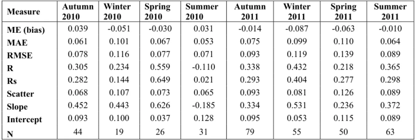
223 224 Measure Autumn 2010 Winter 2010 Spring 2010 Summer 2010 Autumn 2011 Winter 2011 Spring 2011 Summer 2011 ME (bias) 0.039 -0.051 -0.030 0.031 -0.014 -0.087 -0.063 -0.010 MAE 0.061 0.101 0.067 0.053 0.075 0.099 0.110 0.064 RMSE 0.078 0.116 0.077 0.071 0.093 0.119 0.139 0.089 R 0.305 0.234 0.559 -0.110 0.338 0.432 0.218 0.365 Rs 0.282 0.144 0.649 0.021 0.293 0.404 0.277 0.298 Scatter 0.068 0.107 0.073 0.065 0.093 0.081 0.126 0.089 Slope 0.452 0.443 0.626 -0.185 0.334 0.531 0.236 0.372 Intercept 0.093 0.100 0.037 0.128 0.095 0.053 0.115 0.089 N 44 19 26 31 79 55 50 63 225
226
Figure 3: Agreement between in-situ (red) and predicted SSM (blue) from SMOS for the different land
227
cover types throughout 2010 in EUROPE. Results are shown for: (a) ES_AGU and (b) ES_LJU. 228
229
Figure 4: Agreement between in-situ (red) and predicted SSM (blue) from SMOS for the different land
230
cover types throughout 2011 in EUROPE. Results are shown for: (a) ES_AGU and (b) ES_LJU and (c) 231
FR_MAU 232
233 234 235 236 237 238 239 240 241 242 243 244 245 246 247 248 249 250
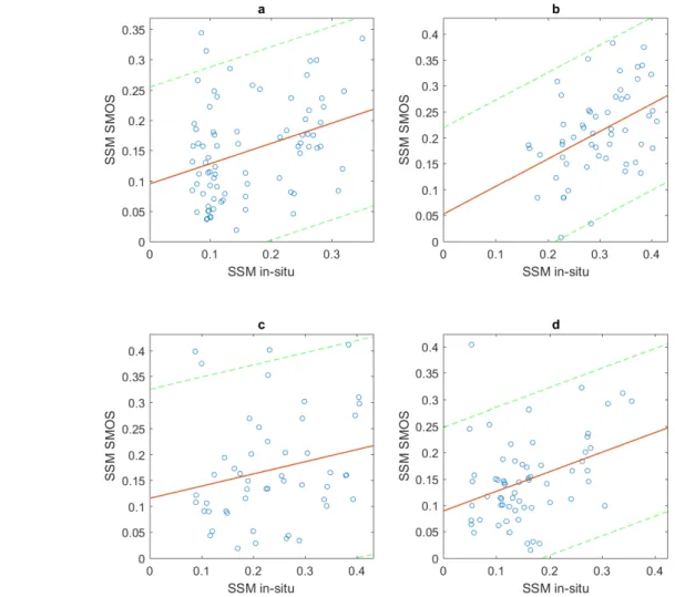
Figure 5: Agreement between in-situ and predicted SSM from SMOS for the different seasons for all
251
sites together shown here for year EUROPE. In particular, for (a) Autumn, (b) Winter, (c) Spring, (d) for 252 2011 253 254 4.2 USA: 255
4.2.1 Comparisons for different land use/cover types
256
A total of four stations were included in the USA. The characteristic land surface cover types in this area 257
are as follows: ME2 stands for Evergreen Needle-leaf Forest (ENF), TON represents Woody Savannahs 258
(WSA), VAR stands for Grasslands (GRA) and WHS represents Open Shrublands (OSH). Table 3 and 259
Figures 6-9 show the comparison statistics between SMOS product and the in-situ measurements over 260
different land cover types. The correlation coefficient of the predicted and the observed measurements is 261
included in the scatterplots (Figure 6). 262
Overall, as indicated from the statistical metrics computed for the analysis of the combination of all sites, 263
a very good agreement between the two datasets was indicated (RMSE = 0.080 m3/m3, bias = 0.014 m3/
264
m3, scatter = 0.079 m3/m3 and R= 0.80). In the case of the different Land cover comparison, SMOS
product had negative bias over ME2 (ENF) and TON (WSA), while the positive bias over VAR (GRA) 266
and WHS (OSH) for both 2010 and 2011. In term of correlation coefficient, SMOS product performance 267
was good for all sites except ME2 (ENF) which has minimum correlation coefficient for RME2 _2010 =
268
0.116 reflected by the RMSE=0.117, in contrast to the high performance in 2011 for the same site 269
(RME2_2011 =0.759, RMSE=0.040). In addition, SMOS product shows maximum scatter (or standard
270
deviation) on ME22010 (Scatter = 0.110), while the scattering is minimum in ME22011 (Scatter = 0.031).
271
Moreover, the product has shown small RMSE values (all between 0.040 and 0.117), illustrating 272
preferable correlation to the in-situ measurements. In addition, the SMOS products for TON, VAR and 273
WHS showed good data quality in terms of accuracy, stability, and correlation coefficient over the 274
different land cover types in USA, as seen in the scatter plots of Figure 7. In contrast SMOS product over 275
Evergreen Needle-forest ME2could not effectively coincide with the in-situ measurements (Figure 7: (i)-276
a and (ii)-a) displaying either very high or very low slope and high intercept. 277
278
Table 3: Comparison between Satellite (SMOS) and observed SSM at the validation sites in USA based
279
on land cover type, for 2010 and 2011 as well as all sites (both years). ME2 stands for Evergreen Needle-280
leaf Forest, TON represents Woody Savannahs, VAR stands for Grasslands and WHS represents Open 281
Shrublands. Units are in m3/m3
282 Measure ME2 2010 ME2 2011 TON 2010 TON 2011 VAR 2010 VAR 2011 WHS 2010 WHS 2011 All Sites ME (bias) -0.045 -0.025 -0.033 -0.016 0.047 0.073 0.074 0.082 0.014 MAE 0.089 0.033 0.054 0.055 0.051 0.077 0.075 0.082 0.062 RMSE 0.117 0.040 0.075 0.068 0.065 0.093 0.086 0.092 0.080 R 0.116 0.759 0.890 0.875 0.947 0.842 0.616 0.682 0.803 Rs 0.232 0.276 0.840 0.849 0.913 0.845 0.528 0.629 0.736 Scatter 0.110 0.031 0.068 0.067 0.046 0.059 0.045 0.042 0.079 Slope 0.176 2.036 0.768 0.758 1.238 1.406 1.014 1.436 0.789 Intercept 0.079 -0.116 0.024 0.046 0.008 -0.022 0.073 0.068 0.050 N 31 29 61 46 58 28 31 29 313 283
Figure 6: Agreement between in-situ and predicted SSM from SMOS for all the different land cover
284
types in USA. Results are shown for US_ME2 (black), US_TON (red), US_VAR (green) and US_WHS 285
(blue): a) 2010 b) 2011 286
i- 287 288 289 290 291 292 293 294 295 296 297 298 299 300 ii- 301 302
303
Figure 7: Agreement between in-situ and predicted SSM from SMOS for the different land cover types in
304
USA. Results are shown for (a) US_ME2, (b) US_TON, (c) US_VAR and (d) US_WHS. i- 2010 ii- 2011 305
306
4.2.2 Temporal Variability
307
Figure 8 shows the temporal fitting trend between the in-situ measurements (red) and the predicted SSM 308
(blue) over TON (Woody Savannahs), VAR (Grasslands) and WHS (Open Shrublands). For ME2 in 2010 309
and for all sites in 2011, the data were discontinuous with large gaps so the temporal fitting was not 310
included. Even for the remaining sites, in some cases there was a small number of data per month leading 311
to wide confidence margins. Thus, it is not always possible to have results for overestimation or 312
underestimation in a given month with statistical certainty. 313
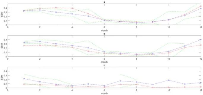
SMOS SSM estimations for TON (Woody Savannahs) is in good agreement with in-situ SSM from May 314
to December with statistically significant underestimation for March and April. For VAR (Grasslands, 315
figure 8b) and WHS (Shrublands, figure 8c), a slight (and not always statistically significant) 316
overestimation of the SSM by SMOS can be witnessed throughout the year. 317
Table 4 summarizes the comparisons between the seasons and Figure 9 shows the agreement between 318
SSM SMOS and the in-situ measurements for the different seasons separately for 2010 and 2011. In 319
general, the SSM SMOS product has shown low RMSE in all the seasons as shown in Table 4 and Figure 320
9. However, the correlation coefficient R was inferior in autumn 2011 and for both summers and 321
generally good in the other seasons in both years. RMSE has the highest values in winter in both years. 322
Spring of 2011 has the highest Pearson’s coefficient from all sites investigated in all continents and the 323
lowest bias 0.012 m3/m3. 324
Table 4: Comparison per season between Satellite (SMOS) and observed SSM at all validation sites in
325
USA for 2010 and 2011. Units are in m3/m3 326
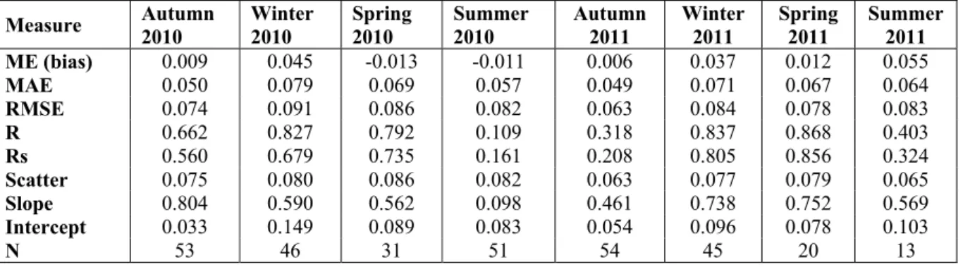
Measure Autumn 2010 Winter 2010 Spring 2010 2010 Summer Autumn 2011 Winter 2011 Spring 2011 Summer 2011
ME (bias) 0.009 0.045 -0.013 -0.011 0.006 0.037 0.012 0.055 MAE 0.050 0.079 0.069 0.057 0.049 0.071 0.067 0.064 RMSE 0.074 0.091 0.086 0.082 0.063 0.084 0.078 0.083 R 0.662 0.827 0.792 0.109 0.318 0.837 0.868 0.403 Rs 0.560 0.679 0.735 0.161 0.208 0.805 0.856 0.324 Scatter 0.075 0.080 0.086 0.082 0.063 0.077 0.079 0.065 Slope 0.804 0.590 0.562 0.098 0.461 0.738 0.752 0.569 Intercept 0.033 0.149 0.089 0.083 0.054 0.096 0.078 0.103 N 53 46 31 51 54 45 20 13 327
328 329
Figure 8: Agreement between in-situ (red) and predicted SSM (blue) from SMOS for the different land
330
cover types throughout 2010 in the USA. Results are shown for: (a) US_TON, (b) US_VAR and (c) 331 US_WHS 332 333 i) 334 335 336 337 338 339 340 341 342 343 344 345 346 347 348
349 ii) 350 351 352 353 354 355 356 357 358 359 360 361 362 363 364 365
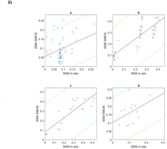
Figure 9: Agreement between in-situ and predicted SSM from SMOS for the different seasons for all
366
sites together shown here for year USA. In particular, for (a) Autumn, (b) Winter, (c) Spring, (d) Summer 367
[ii] 2010 and [ii] 2011
368 369
5. Discussion
370
In this study, SSM SMOS operational product is evaluated using in-situ measurements in two continental 371
regions based on different land cover types. Three in-situ networks in Europe that included: AGU 372
(Shrublands), LJU (olive orchards) and MAU (croplands). In USA four in-situ networks were used 373
namely: ME2 (Evergreen Needle-leaf Forest), TON (Woody Savannahs), VAR (Grasslands) and WHS 374
(Open Shrublands). The performance was evaluated using metrics defined in previous work (Petropoulos 375
et al. 2013). Results are shown in section 4. In this section, an extended discussion is conducted on SMOS 376
SSM product overall performance on different land cover types in order to further improve the algorithm. 377
To summarize, SMOS SSM product is generally applicable in all the selected areas. As shown in Tables 378
1-4, several errors metrics e.g. RMSE, Bias, Scatter, and R showed satisfactory accuracy over selected 379
sites in Europe and USA. In Europe, SMOS SSM has shown reasonable R values, except over the Open 380
Shrubland of AGU2011. This could be due to number of factors such as the retrieved SMOS SSM product
381
observed at a depth of 0-5 cm, whereas in-situ measurement sensors observed at 5 cm. Thus, the strong 382
response to wet and dry period at shallow depth could be a reasonable explanation for discrepancies in 383
agreement (Petropoulos et al. 2013). The SMOS values usually range between (0.001–0.7 m3 m-3),
384
although the values generally presented a dry bias, which causes an underestimation. There is not strong 385
evidence suggesting systematic overestimation or underestimation of SSM by SMOS. This result is 386
coincident with some previous studies that have validated SMOS (Petropoulos et al. 2014). Recent 387
studies (Gumuzzio et al. 2016; Cui et al. 2017) have suggested that the error in SMOS could be due to 388
lack of scale representation between SMOS and the in-situ observations of surface temperature, land 389
cover information, soil condition in particular and the RFI. 390
Previous studies focusing on the product comparisons at the annual scale shows that soil moisture 391
estimates are driven to a certain extent by the seasonal cycle (Qin et al. 2013; Petropoulos et al. 2018b). In 392
our study, in several cases of the seasonal cycle investigation there was a slight underestimation of SSM 393
by SMOS. The negative correlation in summer can be explained mainly by lack of spatial sampling 394
between predicted and observed comparison (Al Bitar et al. 2012). Also, it can be partially attributed to 395
lesser fractional vegetation cover than other seasons and/or could be associated with the smaller sample 396
size than other seasons. On the temporal series comparisons, the predicted SMOS SSM product often 397
overestimates slightly the in-situ observations from May to June or August. This could be explained by 398
the presence of dew which is most prominent during summer, spring and autumn, respectively (De Jeu et 399
al. 2005; Du et al. 2012). In winter, SMOS predictions have low accuracy for European sites and perform 400
very well in USA sites. As such, no conclusions about the performance of SMOS in winter can be made 401
from our study. Summer correlation coefficient is generally suboptimal compared to other seasons for 402
both 2010 and 2011 for USA and European sites. 403
In the USA sites SMOS showed good agreement between the two datasets. In term of correlation 404
coefficient, SMOS product performance was good for TON (WSA), VAR (GRA), and WHS (OSH) in 405
2010 and 2011, but underperformed for ME22010 (ENF). In the case of the different vegetation cover
406
comparison, SMOS product had negative bias over ME2 (ENF) and TON (WSA). The product had 407
positive bias over VAR (GRA) and WHS (OSH) in both years 2010 & 2011. Studies linked SMOS errors 408
to global parameters such as soil texture, RFI, and land cover suggested that globally the forest presence 409
in the radiometer field of view appears to have the great influence on SMOS error up to (56.8%) whereas 410
1.7% of the RFI. The extent of the impact varies among different continents; however, soil texture was 411
highlighted as the main influence over Europe whereas RFI had the greatest influence over Asia. 412
Additionally, a land cover difference as a result of spatial heterogeneity could increase the error in SM 413
within a 0.25◦-resolution pixel. Whereas, forest as well dense vegetation could increase the SSM error by 414
negatively affecting microwave penetration (Rotzer et al. 2012; Leroux et al. 2013; Liu et al. 2018) 415
The Correlation coefficient (R) was inferior in summer and good for winter and spring for both 2010 and 416
2011. In both years RMSE has high values in winter. This could be due to the frozen soil. During summer 417
and spring the error could partially be explained by the presence of dew which has a significant effect on 418
passive microwave observations by increasing horizontal brightness, and is most prominent during 419
summer, spring, and autumn, respectively (De Jeu et al. 2005; Du et al. 2012). RFI can be defined as the 420
disturbance that affects an electromagnetic radiation emitted from an external source (Murray 2013). It is 421
a major problem in SMOS SSM retrieval, which decreases the efficiency of retrieved soil moisture 422
(Jackson et al. 1999). These disturbances largely reduce or limit the quality of the data. Hence, signal 423
contamination removal in L-band is an ongoing research challenge in Europe and many other parts of the 424
world (Kerr et al. 2012; Oliva et al. 2012; Daganzo-Eusebio et al. 2013). 425
Overall, the lack of agreement between the predicted and observed SSM for all scenarios examined here 426
can be attributed to a number of factors, such as: (1) the topographic and vegetation properties complexity. 427
It is known that high vegetation density (e.g., taller and/or denser), frozen soils, snow cover, and volume 428
scattering in dry soils are very critical for SSM operational products retrieval accuracy (Brocca et al. 429
2017). With regards to vegetation effects in particular the quality of SSM retrievals could be strongly 430
affected by the vegetation structure and water content. (2) The differences in terms of the SSM sensing 431
depth between the compared datasets. In our study the surface ground measurement used for the 432
evaluation is at 5cm. while the sampling depth of the effective soil moisture of SMOS varies as a function 433
of topography and land cover characteristics (Deng et al. 2019). (3) Differences in spatial observation 434
scale. Since the exact scale of the satellite observation could not be represented by ground observation, 435
the average point-based measurement is used as a “reference”. However, as is also argued in many studies, 436
it is difficult to characterize the spatial soil moisture patterns by using in-situ measurement. It is able only 437
to reproduce the temporal dynamic of soil moisture but not the absolute value (Petropoulos et al. 2015). 438
Sometimes, if in-situ sensors are not dense enough, it causes mismatch in scales and hence poor accuracy 439
in comparison. (4) Errors caused by measurements accuracy of the sensors Land surface factors, such as 440
topography, seasons and land cover types (particularly at the presence of forests) have been pointed out as 441
elements to affect the product accuracy and consistency. In addition to that they affect the quality of the 442
product that can be expected by the final user (Dorigo et al. 2013; Petropoulos et al. 2014). 443
6. Conclusions – Future work
444
The quantification of the SMOS SSM product accuracy is crucial for hydrological applications of the 445
product and for the retrieval algorithm refinement. This study explores the performance of the SMOS 446
product. SMOS data were compared to in-situ measurements from FLUXNET validated observational 447
networks over different land cover, seasonal and varied climatic zones. This comparison increases our 448
understanding to the product application at continental expanse. SMOS product is available for a long 449
term period that can be used in modeling of scale-related researches such as land surface and hydrological 450
studies. On the other hand the present evaluation can provide help and feedback for the current retrieval 451
algorithm improvement. 452
The study results showed that direct comparison of SMOS operational product with in-situ observations 453
indicate good performance of the product within these sites in respect of the RMSE. The main findings of 454
the study can be summarized as follows: 455
(1) The overall comparison at variety of sites showed generally reasonable agreement between the 456
SMOS product and the in-situ measurement of soil moisture, but at different vegetation cover, 457
some SMOS observations show negative bias. The results were largely comparable to pervious 458
related validation studies. 459
(2) The agreement between the in-situ measurements and the product SSM estimations is 460
observed in regard to different vegetation covers, where SMOS product displayed negative 461
bias over ME2 (ENF) and TON (WSA), while the positive bias over VAR (GRA) and WHS 462
(OSH). This conclusion suggests that the vegetation effects must be carefully accounted for 463
consistent SSM estimations. SMOS uses nadir optical depth and different polarization 464
incidence angle to estimate vegetation optical depth. Land cover impacts the variation of soil 465
moisture content because of increasing transpiration losses and rainfall interception. 466
Furthermore, the type of land cover also influences the vegetation attenuation and scattering 467
albedo which can affect the overall soil moisture retrieval. Therefore, analyzing the effect of 468
vegetation on these algorithms would be important. 469
(3) The seasonal periods where the predicted and observed SSM exhibited low correlation 470
coefficient are summer and autumn. This could partially be explained by the presence of dew 471
which is most prominent during summer, spring and autumn. Seasonality is one of the major 472
controls on soil moisture dynamic and its variability can have very important impacts which 473
can influence overall performance of the soil moisture retrieval. 474
The work presented was focused on temperate areas. As the results were promising, work is ongoing in 475
expanding the SMOS SSM, SMAP, ASCAT operational SSM product evaluation over cold and arid 476
regions. The effect of vegetation cover factor that affects the data quality mentioned in the previous 477
paragraphs will be comprehensively considered. In the future, the integration of numerical weather 478
models, meteorological variables, local hydrological models and information on land cover could also be 479
utilized to more accurately analyze the effect of seasonality on soil moisture estimation as already 480
demonstrated in other studies (Srivastava et al. 2013). 481
482
Acknowledgements
483
The contribution of DKAK and YB was supported by Projects of International Cooperation and 484
Exchanges NSFC (NSFC-RCUK_STFC) (61661136005), the National Key Research and development 485
Program of China (2016YFA0600703), “Six Talents Peak” high-level talent project in Jiangsu Province 486
(2015-JY-013), and Projects of Key Laboratory of Radiometric Calibration and Validation for 487
Environmental Satellites National Satellite Meteorological Center, China Meteorological Administration. 488
GPP’s contribution has been supported by the FP7- People project ENViSIoN-EO (project reference 489
number 752094) and SL’s by the High Performance Computing Wales (HPCW) TRANSFORM-EO 490
project. Sincere thanks also go to Matthew North who helped to conduct the research. Authors wish to 491
thank EUMETSAT for the provision of the SMOS satellite data and also the FLUXNET network for the 492
provision of the in-situ data used in the present study. 493
Author Contributions
494
Methodology Development, Data Acquisition, Analysis: all co-authors; Writing: lead by KAKD with 495
contributions also from all other co-authors. 496
497
References
498
Baldocchi, D D, R Valentini, S Running, W Oechel, and R Dhalman. 1995. “Strategies for Measuring and 499
Modeling CO2 and Water Vapor Fluxes over Terrestrial Ecosystems.” Global Change Biology 500
(Submitted) 2: 159–168.
501
Bao, Yansong, Libin Lin, Shanyu Wu, Khidir Abdalla Kwal Deng, and George P. Petropoulos. 2018. 502
“Surface Soil Moisture Retrievals over Partially Vegetated Areas from the Synergy of Sentinel-1 503
and Landsat 8 Data Using a Modified Water-Cloud Model.” International Journal of Applied Earth 504
Observation and Geoinformation 72 (October): 76–85. https://doi.org/10.1016/j.jag.2018.05.026.
505
Bitar, Ahmad Al, Delphine Leroux, Yann H. Kerr, Olivier Merlin, Philippe Richaume, Alok Sahoo, and 506
Eric F. Wood. 2012. “Evaluation of SMOS Soil Moisture Products Over Continental U.S. Using the 507
SCAN/SNOTEL Network.” IEEE Transactions on Geoscience and Remote Sensing 50 (5): 1572–86. 508
https://doi.org/10.1109/TGRS.2012.2186581. 509
Bittelli, Marco, Roberto Valentino, Fiorenzo Salvatorelli, and Paola Rossi Pisa. 2012. “Monitoring Soil-510
Water and Displacement Conditions Leading to Landslide Occurrence in Partially Saturated Clays.” 511
Geomorphology 173–174 (November): 161–73. https://doi.org/10.1016/j.geomorph.2012.06.006.
512
Brocca, Luca, Luca Ciabatta, Christian Massari, Stefania Camici, and Angelica Tarpanelli. 2017. “Soil 513
Moisture for Hydrological Applications: Open Questions and New Opportunities.” Water 9 (2): 140. 514
https://doi.org/10.3390/w9020140. 515
Brocca, Luca, Wade T. Crow, Luca Ciabatta, Christian Massari, Patricia de Rosnay, Markus Enenkel, 516
Sebastian Hahn, et al. 2017. “A Review of the Applications of ASCAT Soil Moisture Products.” 517
IEEE Journal of Selected Topics in Applied Earth Observations and Remote Sensing 10 (5): 2285–
518
2306. https://doi.org/10.1109/JSTARS.2017.2651140. 519
Calvet, Jean-Christophe, Jean-Pierre Wigneron, Jeffrey Walker, Fatima Karbou, André Chanzy, and 520
Clément Albergel. 2011. “Sensitivity of Passive Microwave Observations to Soil Moisture and 521
Vegetation Water Content: L-Band to W-Band.” IEEE Transactions on Geoscience and Remote 522
Sensing 49 (4): 1190–99. https://doi.org/10.1109/TGRS.2010.2050488.
523
Canone, D., M. Previati, I. Bevilacqua, L. Salvai, and S. Ferraris. 2015. “Field Measurements Based 524
Model for Surface Irrigation Efficiency Assessment.” Agricultural Water Management 156 (July): 525
30–42. https://doi.org/10.1016/j.agwat.2015.03.015. 526
Canone, Davide, Maurizio Previati, and Stefano Ferraris. 2017. “Evaluation of Stemflow Effects on the 527
Spatial Distribution of Soil Moisture Using TDR Monitoring and an Infiltration Model.” Journal of 528
Irrigation and Drainage Engineering 143 (1): 04016075.
https://doi.org/10.1061/(ASCE)IR.1943-529
4774.0001120. 530
Chakravorty, Aniket, Bhagu Ram Chahar, Om Prakash Sharma, and C. T. Dhanya. 2016. “A Regional 531
Scale Performance Evaluation of SMOS and ESA-CCI Soil Moisture Products over India with 532
Simulated Soil Moisture from MERRA-Land.” Remote Sensing of Environment 186: 514–27. 533
https://doi.org/10.1016/j.rse.2016.09.011. 534
Chen, Fan, Wade T. Crow, Rajat Bindlish, Andreas Colliander, Mariko S. Burgin, Jun Asanuma, and 535
Kentaro Aida. 2018. “Global-Scale Evaluation of SMAP, SMOS and ASCAT Soil Moisture 536
Products Using Triple Collocation.” Remote Sensing of Environment 214 (September): 1–13. 537
https://doi.org/10.1016/j.rse.2018.05.008. 538
Crow, Wade T., Aaron A. Berg, Michael H. Cosh, Alexander Loew, Binayak P. Mohanty, Rocco 539
Panciera, Patricia de Rosnay, Dongryeol Ryu, and Jeffrey P. Walker. 2012. “Upscaling Sparse 540
Ground-Based Soil Moisture Observations for the Validation of Coarse-Resolution Satellite Soil 541
Moisture Products.” Reviews of Geophysics 50 (2): RG2002. 542
https://doi.org/10.1029/2011RG000372. 543
Cui, Huizhen, Lingmei Jiang, Jinyang Du, Shaojie Zhao, Gongxue Wang, Zheng Lu, and Jian Wang. 544
2017. “Evaluation and Analysis of AMSR-2, SMOS, and SMAP Soil Moisture Products in the 545
Genhe Area of China.” Journal of Geophysical Research: Atmospheres 122 (16): 8650–66. 546
https://doi.org/10.1002/2017JD026800. 547
Daganzo-Eusebio, Elena, Roger Oliva, Yann H. Kerr, Sara Nieto, Philippe Richaume, and Susanne 548
Martha Mecklenburg. 2013. “SMOS Radiometer in the 1400–1427-MHz Passive Band: Impact of 549
the RFI Environment and Approach to Its Mitigation and Cancellation.” IEEE Transactions on 550
Geoscience and Remote Sensing 51 (10): 4999–5007. https://doi.org/10.1109/TGRS.2013.2259179.
551
Das, N.N., Dara Entekhabi, S. Kim, S. Yueh, R. S. Dunbar, and A. Colliander. n.d. 2017. 552
“SMAP/Sentinel-1 L2 Radiometer/Radar 30-Second Scene 3 Km EASE-Grid Soil Moisture, 553
Version 1.” https://doi.org/10.5067/ZRO7EXJ8O3XI. 554
Deng, Khidir, Salim Lamine, Andrew Pavlides, George Petropoulos, Prashant Srivastava, Yansong Bao, 555
Dionissios Hristopulos, and Vasileios Anagnostopoulos. 2019. “Operational Soil Moisture from 556
ASCAT in Support of Water Resources Management.” Remote Sensing 11 (5): 579. 557
https://doi.org/10.3390/rs11050579. 558
Djamai, Najib, Ramata Magagi, Kalifa Goïta, Mehdi Hosseini, Michael H. Cosh, Aaron Berg, and Brenda 559
Toth. 2015. “Evaluation of SMOS Soil Moisture Products over the CanEx-SM10 Area.” Journal of 560
Hydrology 520: 254–67. https://doi.org/10.23919/EUSIPCO.2017.8081611.
561
Dorigo, W.A., A. Xaver, M. Vreugdenhil, A. Gruber, A. Hegyiová, A.D. Sanchis-Dufau, D. Zamojski, et 562
al. 2013. “Global Automated Quality Control of In Situ Soil Moisture Data from the International 563
Soil Moisture Network.” Vadose Zone Journal 12 (3): 0. https://doi.org/10.2136/vzj2012.0097. 564
Draper, C. S., R. H. Reichle, G. J.M. De Lannoy, and Q. Liu. 2012. “Assimilation of Passive and Active 565
Microwave Soil Moisture Retrievals.” Geophysical Research Letters 39 (4): n/a-n/a. 566
https://doi.org/10.1029/2011GL050655. 567
Du, Jinyang, Thomas J. Jackson, Rajat Bindlish, Michael H. Cosh, Li Li, Brian K. Hornbuckle, and Erik 568
D. Kabela. 2012. “Effect of Dew on Aircraft-Based Passive Microwave Observations over an 569
Agricultural Domain.” Journal of Applied Remote Sensing 6 (1): 63571. 570
https://doi.org/10.1117/1.JRS.6.063571. 571
Fascetti, F., N. Pierdicca, L. Pulvirenti, and R. Crapolicchio. 2014. “ASCAT and SMOS Soil Moisture 572
Retrievals: A Comparison over Europe and Northern Africa.” 13th Specialist Meeting on Microwave 573
Radiometry and Remote Sensing of the Environment, MicroRad 2014 - Proceedings 45: 10–13.
574
https://doi.org/10.1109/MicroRad.2014.6878898. 575
González-Zamora, Ángel, Nilda Sánchez, José Martínez-Fernández, Ángela Gumuzzio, María Piles, and 576
Estrella Olmedo. 2015. “Long-Term SMOS Soil Moisture Products: A Comprehensive Evaluation 577
across Scales and Methods in the Duero Basin (Spain).” Physics and Chemistry of the Earth 83–84: 578
123–36. https://doi.org/10.1016/j.pce.2015.05.009. 579
Grings, Francisco, Cintia A. Bruscantini, Ezequiel Smucler, Federico Carballo, María Eugenia Maria 580
Eugenia Dillon, Estela Angela Collini, Mercedes Salvia, and Haydee Karszenbaum. 2015. 581
“Validation Strategies for Satellite-Based Soil Moisture Products Over Argentine Pampas.” IEEE 582
Journal of Selected Topics in Applied Earth Observations and Remote Sensing 8 (8): 4094–4105.
583
https://doi.org/10.1109/JSTARS.2015.2449237. 584
Gumuzzio, A., L. Brocca, N. Sánchez, A. González-Zamora, and J. Martínez-Fernández. 2016. 585
“Comparison of SMOS, Modelled and in Situ Long-Term Soil Moisture Series in the Northwest of 586
Spain.” Hydrological Sciences Journal. https://doi.org/10.1080/02626667.2016.1151981. 587
Jackson, T.J., D.M. Le Vine, A.Y. Hsu, A. Oldak, P.J. Starks, C.T. Swift, J.D. Isham, and M. Haken. 588
1999. “Soil Moisture Mapping at Regional Scales Using Microwave Radiometry: The Southern 589
Great Plains Hydrology Experiment.” IEEE Transactions on Geoscience and Remote Sensing 37 (5): 590
2136–51. https://doi.org/10.1109/36.789610. 591
Jeu, Richard A. M. De, Thomas R. H. Holmes, and Manfred Owe. 2005. “Determination of the Effect of 592
Dew on Passive Microwave Observations from Space.” In Geophysical Research Abstracts 7: 593
04001, edited by Manfred Owe and Guido D’Urso, 597608. https://doi.org/10.1117/12.627919.
594
Kerr, Y.H., Waldteufel, P., Wigneron, J.-P., Martinuzzi, J., Font, J., Berger, M. 2001. “Soil Moisture 595
Retrieval from Space: The Soil Moisture and Ocean Salinity (SMOS) Mission.” IEEE Trans. Geosci. 596
Remote Sens. 39, 1729–1735.
597
Kerr, Yann H., Philippe Waldteufel, Philippe Richaume, Jean Pierre Wigneron, Paolo Ferrazzoli, Ali 598
Mahmoodi, Ahmad Al Bitar, et al. 2012. “The SMOS Soil Moisture Retrieval Algorithm.” IEEE 599
Transactions on Geoscience and Remote Sensing 50 (5): 1384–1403.
600
https://doi.org/10.1109/TGRS.2012.2184548. 601
Leroux, Delphine J., Yann H. Kerr, Philippe Richaume, and Remy Fieuzal. 2013. “Spatial Distribution 602
and Possible Sources of SMOS Errors at the Global Scale.” Remote Sensing of Environment 133 603
(June): 240–50. https://doi.org/10.1016/j.rse.2013.02.017. 604
Liu, Y. Y., R. M. Parinussa, W. A. Dorigo, R. A M De Jeu, W. Wagner, A. I. J. M. van Dijk, M. F. 605
McCabe, and J. P. Evans. 2011. “Developing an Improved Soil Moisture Dataset by Blending 606
Passive and Active Microwave Satellite-Based Retrievals.” Hydrology and Earth System Sciences 607
15 (2): 425–36. https://doi.org/10.5194/hess-15-425-2011. 608
Liu, Yangxiaoyue, Yaping Yang, and Xiafang Yue. 2018. “Evaluation of Satellite-Based Soil Moisture 609
Products over Four Different Continental In-Situ Measurements.” Remote Sensing 10 (7): 1161. 610
https://doi.org/10.3390/rs10071161. 611
Louvet, Samuel, Thierry Pellarin, Ahmad Al Bitar, Bernard Cappelaere, Sylvie Galle, Manuela Grippa, 612
Claire Gruhier, et al. 2015. “SMOS Soil Moisture Product Evaluation over West-Africa from Local 613
to Regional Scale.” Remote Sensing of Environment 156: 383–94. 614
https://doi.org/10.1016/j.rse.2014.10.005. 615
Murray, D. 2013. “Using RF Recording Techniques to Resolve Interference Problems.” 2013 IEEE 616
AUTOTESTCON, Schaumburg, IL, September 16–19 2012, 1–6. IEEE. Doi:10.1109/
617
AUTEST.2013.6645046. https://doi.org/10.1109/ AUTEST.2013.6645046.
618
Oliva, Roger, Elena Daganzo, Yann H. Kerr, Susanne Mecklenburg, Sara Nieto, Philippe Richaume, and 619
Claire Gruhier. 2012. “SMOS Radio Frequency Interference Scenario: Status and Actions Taken to 620
Improve the RFI Environment in the 1400–1427-MHz Passive Band.” IEEE Transactions on 621
Geoscience and Remote Sensing 50 (5): 1427–39. https://doi.org/10.1109/TGRS.2012.2182775.
622
Panciera, Rocco, Jeffrey P. Walker, Jetse Kalma, and Edward Kim. 2011. “A Proposed Extension to the 623
Soil Moisture and Ocean Salinity Level 2 Algorithm for Mixed Forest and Moderate Vegetation 624
Pixels.” Remote Sensing of Environment 115 (12): 3343–54. 625
https://doi.org/10.1016/j.rse.2011.07.017. 626
Petropoulos, G. P., P. K. Srivastava, K. P. Ferentinos, and D. Hristopoulos. 2018a. “Evaluating the 627
Capabilities of Optical/TIR Imaging Sensing Systems for Quantifying Soil Water Content.” 628
Geocarto International, October, 1–18. https://doi.org/10.1080/10106049.2018.1520926.
629
Petropoulos, George, Hywel Griffiths, Wouter Dorigo, Angelika Xaver, and Alexander Gruber. 2013. 630
“Surface Soil Moisture Estimation.” In Remote Sensing of Energy Fluxes and Soil Moisture Content, 631
29–48. CRC Press. https://doi.org/10.1201/b15610-4. 632
Petropoulos, George P., Gareth Ireland, and Brian Barrett. 2015a. “Surface Soil Moisture Retrievals from 633
Remote Sensing: Current Status, Products & Future Trends.” Physics and Chemistry of the 634
Earth, Parts A/B/C 83–84: 36–56. https://doi.org/10.1016/j.pce.2015.02.009.
635
Petropoulos, George P., Gareth Ireland, and Prashant K. Srivastava. 2015b. “Evaluation of the Soil 636
Moisture Operational Estimates From SMOS in Europe: Results Over Diverse Ecosystems.” IEEE 637
Sensors Journal 15 (9): 5243–51. https://doi.org/10.1109/JSEN.2015.2427657.
638
Petropoulos, George P., Gareth Ireland, Prashant K. Srivastava, and Pavlos Ioannou-Katidis. 2014. “An 639
Appraisal of the Accuracy of Operational Soil Moisture Estimates from SMOS MIRAS Using 640
Validated in Situ Observations Acquired in a Mediterranean Environment.” International Journal of 641
Remote Sensing 35 (13): 5239–50. https://doi.org/10.1080/2150704X.2014.933277.
642
Petropoulos, George P., and Jon P. McCalmont. 2017. “An Operational in Situ Soil Moisture & Soil 643
Temperature Monitoring Network for West Wales, UK: The WSMN Network.” Sensors 644
(Switzerland) 17 (7): 1481. https://doi.org/10.3390/s17071481.
645
Petropoulos, George P., Prashant K. Srivastava, Maria Piles, and Simon Pearson. 2018b. “Earth 646
Observation-Based Operational Estimation of Soil Moisture and Evapotranspiration for Agricultural 647
Crops in Support of Sustainable Water Management.” Sustainability (Switzerland) 10 (1): 181. 648
https://doi.org/10.3390/su10010181. 649
Pierdicca, Nazzareno, Luca Pulvirenti, Fabio Fascetti, Raffaele Crapolicchio, Marco Talone, and Silvia 650
Puca. 2012. “Soil Moisture from Satellite: A Comparison of METOP, SMOS and ASAR Products.” 651
Proceedings 2012 EUMETSAT Meteorological Satellite Conference, 1–8.
652
Qin, Jun, Kun Yang, Ning Lu, Yingying Chen, Long Zhao, and Menglei Han. 2013. “Spatial Upscaling of 653
In-Situ Soil Moisture Measurements Based on MODIS-Derived Apparent Thermal Inertia.” Remote 654
Sensing of Environment 138 (November): 1–9. https://doi.org/10.1016/j.rse.2013.07.003.
655
Raffelli, Giulia, Maurizio Previati, Davide Canone, Davide Gisolo, Ivan Bevilacqua, Giorgio Capello, 656
Marcella Biddoccu, et al. 2017. “Local- and Plot-Scale Measurements of Soil Moisture: Time and 657
Spatially Resolved Field Techniques in Plain, Hill and Mountain Sites.” Water 9 (9): 706. 658
https://doi.org/10.3390/w9090706. 659
Ro¨tzer, K., C. Montzka, H. Bogena, W. Wagner, Y.H. H. Kerr, R. Kidd, H. Vereecken, et al. 2014. 660
“Catchment Scale Validation of SMOS and ASCAT Soil Moisture Products Using Hydrological 661
Modeling and Temporal Stability Analysis.” Journal of Hydrology 519 (PA): 934–46. 662
https://doi.org/10.1016/j.jhydrol.2014.07.065. 663
Rosnay, P.; Drusch, M.; Vasiljevic, D.; Balsamo, G.; Albergel, C.; Isaksen, L. A. De, Patricia De Rosnay, 664
Matthias Drusch, Drasko Vasiljevic, Gianpaolo Balsamo, Clément Albergel, and Lars Isaksen. 2013. 665
“Simplified Extended Kalman Filter for the Global Operational Soil Moisture Analysis at ECMWF. 666
Q. J. R.” Meteorol. Soc. 139 (674): 1199–1213. https://doi.org/10.1002/qj.2023. 667
Rotzer, K., C. Montzka, H. Bogena, W. Wagner, R. Kidd, and H. Vereecken. 2012. “Time Series 668
Analysis of SMOS and ASCAT: Soil Moisture Product Validation in the Rur and Erft Catchments.” 669
In 2012 IEEE International Geoscience and Remote Sensing Symposium, 14:3716–19. IEEE. 670
https://doi.org/10.1109/IGARSS.2012.6350510. 671
Sánchez-Ruiz, Sergio, María Mari´a María Piles, Nilda Sánchez, José Martínez-Fernández, Mercè Merce` 672
Vall-llossera, Adriano Camps, Sergio Sa´nchez-Ruiz, et al. 2014. “Combining SMOS with Visible 673
and near/Shortwave/Thermal Infrared Satellite Data for High Resolution Soil Moisture Estimates.” 674
Journal of Hydrology 516 (August): 273–83. https://doi.org/10.1016/j.jhydrol.2013.12.047.
675
Seneviratne, Sonia I., Thierry Corti, Edouard L. Davin, Martin Hirschi, Eric B. Jaeger, Irene Lehner, 676
Boris Orlowsky, and Adriaan J. Teuling. 2010. “Investigating Soil Moisture-Climate Interactions in 677
a Changing Climate: A Review.” Earth-Science Reviews 99 (3–4): 125–61. 678
https://doi.org/10.1016/j.earscirev.2010.02.004. 679
Shi, Jiancheng, Xiaolong Dong, Tianjie Zhao, Jinyang Du, Lingmei Jiang, Yang Du, Hao Liu, Zhenzhan 680
Wang, Dabin Ji, and Chuan Xiong. 2014. “WCOM : THE SCIENCE SCENARIO AND 681
OBJECTIVES OF A GLOBAL WATER CYCLE OBSERVATION MISSION State Key 682
Laboratory of Remote Sensing Science , Institute of Remote Sensing and Digital Earth , Chinese 683
Academy of Sciences CAS Key Laboratory of Microwave Remote Sens,” 3646–49. 684
https://www.mendeley.com/catalogue/wcom-science-scenario-objectives-global-water-cycle-685
observation-mission-state-key-laboratory-remote/. 686
Srivastava, P. K., T. Islam, S. K. Singh, M. Gupta, G. P. Petropoulos, D. K. Gupta, W. Z. Wan Jaafar, and 687
R. Prasad. 2016a. “Soil Moisture Deficit Estimation Through SMOS Soil Moisture and MODIS 688
Land Surface Temperature.” In Satellite Soil Moisture Retrieval: Techniques and Applications, 333– 689
47. Elsevier. https://doi.org/10.1016/B978-0-12-803388-3.00017-6. 690
Srivastava, Prashant K., Dawei Han, Miguel A. Rico-Ramirez, Peggy O’Neill, Tanvir Islam, and Manika 691
Gupta. 2014. “Assessment of SMOS Soil Moisture Retrieval Parameters Using Tau-Omega 692
Algorithms for Soil Moisture Deficit Estimation.” Journal of Hydrology 519 (PA): 574–87. 693
https://doi.org/10.1016/j.jhydrol.2014.07.056. 694
Srivastava, Prashant K., Dawei Han, Miguel A. Rico Ramirez, and Tanvir Islam. 2013. “Appraisal of 695
SMOS Soil Moisture at a Catchment Scale in a Temperate Maritime Climate.” Journal of Hydrology 696
498 (August): 292–304. https://doi.org/10.1016/j.jhydrol.2013.06.021. 697
Srivastava, Prashant K., George P. Petropoulos, Yann H. Kerr, Yann H. Kerr Prashant K. Srivastava, 698
George P. Petropoulos, Prashant K. Srivastava, George P. Petropoulos, and Yann H. Kerr. 2016b. 699
Satellite Soil Moisture Retrieval : Techniques and Applications. Elsevier.
700
http://www.sciencedirect.com/science/book/9780128033883. 701
Vereecken, H., J. A. Huisman, H. Bogena, J. Vanderborght, J. A. Vrugt, and J. W. Hopmans. 2008. “On 702
the Value of Soil Moisture Measurements in Vadose Zone Hydrology: A Review.” Water Resources 703
Research 44 (4): 1–21. https://doi.org/10.1029/2008WR006829.
704
Wanders, N., D. Karssenberg, A. De Roo, S. M. De Jong, and M. F P Bierkens. 2014. “The Suitability of 705
Remotely Sensed Soil Moisture for Improving Operational Flood Forecasting.” Hydrology and 706
Earth System Sciences 18 (6): 2343–57. https://doi.org/10.5194/hess-18-2343-2014.
707
Zhuo, Lu, Qiang Dai, and Dawei Han. 2015. “Evaluation of SMOS Soil Moisture Retrievals over the 708
Central United States for Hydro-Meteorological Application.” Physics and Chemistry of the Earth, 709
Parts A/B/C 83–84: 146–55. https://doi.org/10.1016/j.pce.2015.06.002.
710