HAL Id: hal-02929027
https://hal.inrae.fr/hal-02929027
Submitted on 3 Sep 2020
HAL is a multi-disciplinary open access
archive for the deposit and dissemination of
sci-entific research documents, whether they are
pub-lished or not. The documents may come from
teaching and research institutions in France or
abroad, or from public or private research centers.
L’archive ouverte pluridisciplinaire HAL, est
destinée au dépôt et à la diffusion de documents
scientifiques de niveau recherche, publiés ou non,
émanant des établissements d’enseignement et de
recherche français ou étrangers, des laboratoires
publics ou privés.
biomass derived from management inventories
Pierre Ploton, Frédéric Mortier, Nicolas Barbier, Guillaume Cornu, Maxime
Réjou-Méchain, Vivien Rossi, Alfonso Alonso, Jean-Francois Bastin, Nicolas
Bayol, Fabrice Benedet, et al.
To cite this version:
Pierre Ploton, Frédéric Mortier, Nicolas Barbier, Guillaume Cornu, Maxime Réjou-Méchain, et al..
A map of African humid tropical forest aboveground biomass derived from management inventories.
Scientific Data , Nature Publishing Group, 2020, 7 (1), �10.1038/s41597-020-0561-0�. �hal-02929027�
a map of african humid tropical
forest aboveground biomass
derived from management
inventories
Pierre Ploton
1✉, Frédéric Mortier
2, Nicolas Barbier
1, Guillaume Cornu
2,
Maxime Réjou-Méchain
1, Vivien Rossi
3, alfonso alonso
4, Jean-François Bastin
5,
Nicolas Bayol
6, Fabrice Bénédet
2, Pulchérie Bissiengou
7, Georges Chuyong
8,
Benoît Demarquez
9, Jean-Louis Doucet
10, Vincent Droissart
1,11, Narcisse Guy Kamdem
11,
David Kenfack
12, Hervé Memiaghe
13, Libalah Moses
11, Bonaventure Sonké
11,
Nicolas texier
11,14, Duncan thomas
15, Donatien Zebaze
11, Raphaël Pélissier
1&
Sylvie Gourlet-Fleury
2Forest biomass is key in Earth carbon cycle and climate system, and thus under intense scrutiny in the context of international climate change mitigation initiatives (e.g. REDD+). In tropical forests, the spatial distribution of aboveground biomass (aGB) remains, however, highly uncertain. there is increasing recognition that progress is strongly limited by the lack of field observations over large and remote areas. Here, we introduce the Congo basin Forests aGB (CoFor-aGB) dataset that contains aGB estimations and associated uncertainty for 59,857 1-km pixels aggregated from nearly 100,000 ha of in situ forest management inventories for the 2000 – early 2010s period in five central African countries. a comprehensive error propagation scheme suggests that the uncertainty on aGB estimations derived from c. 0.5-ha inventory plots (8.6–15.0%) is only moderately higher than the error obtained from scientific sampling plots (8.3%). CoFor-AGB provides the first large scale view of forest AGB spatial variation from field data in central Africa, the second largest continuous tropical forest domain of the world.
Background & Summary
Quantifying forest aboveground biomass (AGB) has been the focus of considerable interest in the last century for both commercial (e.g. timber, fiber, energy productions) and scientific (e.g. forest ecosystem functioning and productivity)1 purposes. Nowadays, forest AGB is at the forefront of international research and political agendas
due to its importance in Earth climate system and carbon cycle2,3. While most of global forest AGB is found in
1AMAP, Univ Montpellier, iRD, cnRS, inRAe, ciRAD, Montpellier, france. 2CIRAD, UPR Forêts et Sociétés, F-34398
Montpellier, France; Université de Montpellier, F-34000, Montpellier, France. 3ciRAD, UPR forêts et Sociétés, Yaoundé,
cameroun. 4center for conservation and Sustainability, Smithsonian conservation Biology institute, national Zoological
Park, Washington, Dc, USA. 5cAVeLab computational and Applied Vegetation ecology, Department of Applied ecology
and Environmental Biology, Faculty of Bioscience Engineering, Ghent University, Ghent, 9000, Belgium. 6fRM ingénierie,
34130, Mauguio – Grand Montpellier, France. 7institut de pharmacopée et de médecine traditionnelle (Herbier national
du Gabon), cenAReSt, Libreville, Gabon. 8Department of Plant Science, faculty of Science, University of Buea, Buea,
cameroon. 9Terre Environnement Aménagement, 13001, Marseille, France. 10forest is Life, teRRA teaching and
Research Centre, Gembloux Agro-Bio Tech, University of Liège, Gembloux, Belgium. 11Plant Systematic and ecology
Laboratory (LaBosyste), Department of Biology, Higher teachers’ training college, University of Yaoundé i, P.O. Box 047, Yaoundé, Cameroun. 12ForestGEO, Smithsonian Tropical Research Institute, NMNH - MRC 166, P.O. Box 37012,
Washington, DC, 20013-7012, USA. 13institut de Recherche en ecologie tropicale/centre national de la Recherche
Scientifique et Technologique, Libreville, Gabon. 14faculty of Sciences, evolutionary Biology and ecology, Université
Libre de Bruxelles, CP160/12, 50 Av. F. Roosevelt, 1050, Brussels, Belgium. 15School of Biological Sciences, Washington
State University, 14204 NE Salmon Creek Ave, Vancouver, WA, 98686, USA. ✉e-mail: p.ploton@gmail.com
Data DESCRIPtoR
oPEN
tropical regions4, its spatial distribution within the main tropical forest basins remains subject to large
uncertain-ties, even at regional scale5. This knowledge gap introduces uncertainties into estimates of forest carbon release
from land-use change6,7, and constitutes a major impediment to the design and implementation of climate change
mitigation policies (e.g. Reducing Emissions from Deforestation and forest Degradation, REDD) into countries national development planning. Given the escalation of carbon emissions associated with deforestation8 and
forest degradation9, fires10 and drought events11 in the tropics, it is more than ever important to increase our
understanding of tropical forest AGB geography and of its ecological determinants.
Historically, forest resources assessments have been made through ground inventories12. In temperate
coun-tries where forest management planning is a long-standing tradition, national forest inventories (NFI) have been established early-on and are regularly updated. Across western Europe for instance, today’s sampling intensity is such that it allows visualizing spatial variations of forest AGB from plots AGB estimations alone13, and thus
inferring reliable mean AGB levels at various jurisdictional scales14. In most tropical countries, however, national
forest resources assessment is a more recent practice facing multiple challenges, including limited financial resources, difficulties to access remote regions, and the lack of initial information on forest resource distribution to rationalize any new sampling plan. In the Democratic Republic of Congo for example, which extends on c. 2.345 M.km2 and hosts the majority of the Congo Basin forests, the first NFI was initiated in 2017 and aims at
establishing about 400 sampling units15, while a country like Germany set up more than 40,000 sampling units16
for an area of c. 0.357 M.km2. While DRC’s NFI is a tremendous undertaking and an important step forward for
this country, it is obvious that it will only provide a crude picture of forest AGB spatial distribution. To address the limits of inventory-based estimation methods in such context, a frequent strategy consists of using field sample plots established by research teams (hereafter referred to as scientific plots) to build and validate AGB predic-tion models based on remote sensing and environmental data17,18. Yet again, the representativeness of field plot
estimates generally is a major limit that potentially introduces significant biases in model outputs5. Indeed, large
remote areas are usually unsampled in the tropics so that broad environmental gradients, which may both have an impact on forest AGB and on the remote sensing signal, are not fully represented in these datasets.
Despite pressing needs for field data on tropical forest AGB stocks, management forest inventories have remained overlooked by the scientific and greenhouse gas inventory communities. Since the United Nations sum-mit in Rio de Janeiro (1992), central African countries have begun to revise their forest laws to achieve sustainable forest management, notably making forest management planning mandatory in production forests19. In 2019,
58% of about 50 M.ha of timber logging concessions have been inventoried for management purposes20, with
sampling rates of about 1% depending on countries’ forest laws. These data thus contain information on forest structure and composition over areas that are several orders of magnitude larger than the current extent of scien-tific forest inventories in the region, which hosts the second largest block of continuous tropical forest on Earth.
In this paper, we give access, thanks to the voluntary participation of several logging companies, to nearly 60 thousand 1-km resolution AGB estimates and associated uncertainty spread over contrasted forest types and environmental conditions in five countries from central Africa (Fig. 1). These estimates are based on the aggre-gation of c. 11.8 million measured trees in c. 192,000 field plots, representing an estimated inventory workload of 1000 years for a single person. We validated the AGB computation scheme using data from scientific plots (Fig. 2), allowing a detailed characterization of uncertainty sources and their propagation to plot-level estimations. This dataset thus provides the largest ever published dataset on field-derived tropical forest AGB giving unprecedented information on both the local and regional variability of AGB in tropical forests.
Methods
Data presentation.
Managed concessions forest inventory data. The forest inventory dataset (hereafterCoFor dataset) corresponds to forest management inventories from 114 logging concessions (Fig. 2). Inventories followed standardized protocols22 and were conducted from the early 2000s to the early 2010s, at the exception
of the Ngotto concession (1.4% of the data, sampled in 1993–1996) in the Central African Republic. Sampling designs were systematic and usually consisted of 20 to 25 m wide continuous and parallel transects, located 2 to 3 km apart, that were then aggregated into plots of 0.4 ha (8% of the cases) or 0.5 ha (91.7% of the cases). The remaining 0.3% of the plots ranged between 0.3 and 1 ha. Within each plot, information on tree diameter at breast height (DBH) and taxonomic identity were available for all trees with DBH ≥ 30 cm while smaller trees were either partially sampled or in some cases completely missing (see further). The quality of taxonomic informa-tion has been extensively reviewed elsewhere22. In total, the CoFor dataset contained 191,562 plots, covering a
cumulated sampling area of 94,513 ha and representing 11.82 × 10⁶ tree measurements and 1,091 identified taxa. Scientific forest inventory data. We used scientific forest inventory data to fine-tune and test the AGB
com-putation scheme applied to forest management inventories and described in the next section. Scientific forest data were collated from plot networks and collaborators in Cameroon (IRD plot network23, CTFS Korup24 plot),
Gabon (CTFS Rabi24 plot) and D.R. Congo25 (Fig. 2), and represented 233 1-ha plots. In each plot, the DBH of all
trees with DBH ≥ 10 cm was measured and trees were identified following standard scientific protocols26. Forest
structure in the scientific dataset covered most of the structural range found in CoFor, at the exception of forests characterized by both a small mean tree size and a low tree abundance (Supplementary Fig. 1), likely reflecting degraded forest states which can notably be found in Northern Congo (the so-called Marantaceae forests).
Estimation of plot and pixel aboveground biomass.
Caveats of management inventories in forest concessions. Although the amount of information on central African forests structure and composition in thecompanies do not conform to standard scientific protocols. This entailed additional computation steps and uncer-tainty sources when estimating forest sample plots aboveground biomass (AGB).
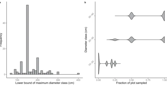
The first limitation of forest management inventories is that tree diameters are recorded as discrete (i.e. by 10 cm width bins), censored data rather than continuously. Tree diameter distributions were right-censored, meaning that all trees above a certain diameter threshold were pooled in a single ‘open class’. This diameter threshold varied across the 114 logging concessions (Fig. 3a) and mainly corresponded to 120 cm, 150 cm or 200 cm (8.9%, 47.8% and 11.5% of the sampling plots, respectively). Since tree AGB allometric models require continuous tree diameter values, it was necessary to establish a strategy to derive continuous DBH values from diameter classes (hereafter specific function 1).
Secondly, while a standard practice in scientific inventory protocols is to census all trees with DBH ≥ 10 cm, this census threshold can be higher in forest management inventory protocols and trees in the smallest diameter classes are not always sampled on the entire plot. In the CoFor dataset, for instance, the tree census threshold was 20 cm DBH in about half of the plots (i.e. 51.6%) and 10 cm DBH otherwise. Trees in the 20–30 and 30–40 cm DBH classes were sampled on the entire plot area in about half of the sampling plots (i.e. 42.7% and 58.4%, respec-tively) and partially sampled, most often on half of the plot area (Fig. 3b), in the remaining cases. When present, information on trees in the 10–20 cm DBH class was the least complete, as it typically corresponded to a sampling of 12.5% up to 33% of the plot area (Fig. 3b). Since forest AGB is commonly reported for all trees ≥ 10 cm DBH in the scientific literature, we developed procedures to correct for the partial inventory (hereafter specific function 2) or complete absence (hereafter specific function 3) of small trees in forest management inventories.
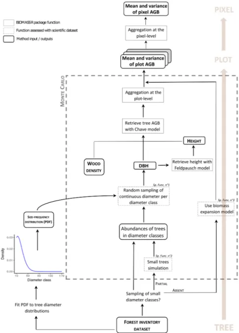
Computation scheme. We built a complete computation scheme to derive standardized estimates of plot AGB
and associated errors from the CoFor dataset using a Monte Carlo approach (see Fig. 4 for a general overview). The general workflow can be decomposed into three main steps. First, forest management inventory data were transformed so as to mimic the format of scientific inventory data, which implied to (i) simulate the abundance of small trees in partially-sampled diameter classes (specific function 2) and (ii) assign continuous tree diameters from discrete diameter classes (specific function 1). Second, we used the BIOMASS R package27 for computing
standardized plot AGB from inventory data using the pantropical AGB allometric model28 and for error
prop-agation. Package’s build-in functions were used to retrieve tree wood density from the Global Wood density database29 and tree height using Feldpausch’s height-diameter allometric model30 parametrized for the central
African region. An estimate of plots AGB was then obtained from trees AGB and either corresponded to the AGB above 10 cm DBH (when trees in the 10–20 cm DBH class were partially sampled in the plot) or above 20 cm DBH (when trees in the 10–20 cm DBH class were not sampled in the plot). In this last case, a third step consisted in applying a correction to plots AGB estimations (i.e. specific function 3) to predict plots AGB above the standard 10 cm DBH threshold.
For each plot, we generated 1000 AGB estimates using a Monte Carlo procedure. For each Monte Carlo sim-ulation, errors associated to each computational step are calculated and propagated throughout the computation chain. This approach has been described elsewhere, notably in the BIOMASS R package27, and is now used as
a standard for generating calibration AGB data for satellite missions31. The procedure outputs a vector of AGB
estimates for each plot (of length 1000 here) from which we extracted the mean and the variance. The mean of
Fig. 1 Overview of the study area in central Africa and field data distribution. Reference forest AGB estimates derived from field inventories, aggregated into 5-km pixels (for visual purpose), are depicted in a green-to-red color gradient and underlaid by the spatial distribution of moist forests21 (grey) and countries borders (black).
AGB estimates within plots was used as the plot AGB value, while the variance and the coefficient of variation (CV) were used to compute estimation uncertainty. Besides classical error sources handled by the BIOMASS R package, an important aspect of our preliminary analyses was to quantify the errors associated to the three specific
functions introduced below to deal with the peculiarities of forest management inventory data and for which we
used scientific forest inventory as test data (see Technical Validation section).
Once computed, plot-level AGB estimates were aggregated into 1-km pixels using the weighted mean function of the SDMTools R package32, with plots area as the set of weights. The resulting 59,857 pixels map represented in
Fig. 1 provides the first overview of large-scale spatial variation in African moist forests AGB derived from field data. Anticipating users’ needs for pixel-level AGB uncertainty assessments, we also computed (i) the weighted mean of within-pixel plots AGB variance (corresponding to intra-plot variance) and (ii) the weighted variance of within-pixel plots mean AGB (corresponding to inter-plot variance). Summing the intra- and inter-plot vari-ances yields pixel-level total variance, which we expressed as a coefficient of variation (in %) to report on the total AGB uncertainty at the pixel scale. Intra- and inter-plot variances were also separately expressed as coefficients of variation (in %), and are hereafter referred to as estimation uncertainty and sampling uncertainty, respectively.
Specific function 1: assignment of tree diameters from diameter classes. Assigning continuous tree diameter values
from a discrete, censored distribution requires positing (i) a probability distribution function (PDF) for contin-uous tree diameters within each diameter class and (ii) the maximum diameter (Dmax) a tree may reach in the
open diameter class (e.g. 150–Dmax cm). In preliminary testing, we used the forest management inventory
data-set to fit three probability distribution functions, namely an exponential distribution, a two-parameter Weibull
Fig. 2 Spatial distribution of forest inventory data in managed concessions of central Africa. (a) Inventory data are colored by logging concessions and aggregated into 5-km pixels (for visual purpose). Black dots represent the location of scientific plots used to evaluate the biomass computation scheme, with dots’ size corresponding to the number of plots per sampling site. Forestry data is underlaid by the spatial distribution of moist forests21 (light grey) and national limits (black). Outlined region is expanded in b. (b) Selected subset of forest
management inventory data colored by logging concessions and displayed at the actual scale of CoFor-AGB, i.e. 1 km. Outlined region is expanded in c. (c) Forest management inventory plots (black dots) along inventory transects, underlaid by the 1-km pixel grid used to aggregate inventory data and compute forest biomass.
distribution and a two-parameter Gamma distribution, each time considering a set of realistic Dmax values (i.e.
from 300 to 500 cm by 50 cm steps). Distribution functions were fitted either by genus or considering all genera simultaneously. A weighted AIC was used to select the distribution that best fitted the data. We then assessed how well these different strategies (i.e. genus-specific or generic PDFs, distribution function type) allowed estimating actual plot AGB using the set of scientific forest plots. Continuous tree diameters in the scientific inventory data-set were discretized, and we used the fitted PDFs to generate continuous tree diameter by inverse transform sam-pling33. We then compared plot AGB estimates derived from degraded and original data. Based on 1000 iterations
of the Monte Carlo scheme on the scientific dataset, we found that Dmax value had little influence on the results
and that using genus-specific PDFs rather than a single generic PDF did not significantly reduce AGB estimation errors. In the final AGB computation scheme (Fig. 4), we thus arbitrarily set Dmax to 400 cm and selected the best
generic PDF, i.e. the 2-parameter Weibull distribution function, with a scale parameter λ = 8.593 and a shape parameter k = 0.737.
Specific function 2: simulation of small tree data in partially-sampled diameter classes. Forest management
inven-tory data often contain a partial sampling of trees in the smallest diameter classes, i.e. trees in diameter class i are sampled in a spatial fraction p of the plots, with i and p varying across logging companies (Fig. 3b). To compute plot AGB for all trees ≥ 10 cm DBH, it was necessary to account for trees that were not sampled. Here, we devel-oped a two-step procedure to simulate missing tree data: at each iteration of the plot AGB Monte Carlo compu-tation, we (i) expanded the tree count r observed in a given diameter class and plot from the spatial fraction p to the entire plot by randomly generating a value from a negative binomial distribution X ~ NegBin(r, p), and (ii) assigned species labels to simulated trees at the pro-rata of species abundance observed in the p fraction of the plot.
Specific function 3: biomass correction model for trees in diameter class 10–20 cm. To predict the total biomass
of plots where trees in diameter class 10–20 cm were not sampled, we developed a biomass correction model using c. 90,000 forest management plots where trees in the 10–20 cm diameter class were partially sampled. In preliminary testing, we first computed AGB of trees in the 10–20 cm diameter class (AGB10–20) and above 20 cm
(AGB≥20) for each plot, as the average of 1000 AGB simulations while propagating classical errors (on wood
density, height-diameter and AGB allometric models) as well as errors on the simulation of small trees and diam-eter assignment functions inherent to our AGB Monte Carlo computation scheme. Across forest management plots, AGB10-20 represented on average 10.1 ± 8.6% of AGB≥20, close to what was found on the scientific dataset
(11.3 ± 7.9%). Then, we tested several simple linear models to predict AGB10-20, using the set of 90,000 plots as
calibration data and scientific plots as validation data. Using AGB≥20 as sole model predictor led to a poor
cali-bration fit (R²calib. of 0.04, Fig. S5a) and predictive power (R²valid. of 0.02 on scientific plots). In order to improve
the AGB10-20 model, we thus computed two additional metrics, S and I, describing the shape of plots cumulated
biomass distribution function (Fig. 5b). S and I correspond respectively to the slope and the intercept of a simple
0 20 40
100 200 300 400
Lower bound of maximum diameter class (cm)
Frequenc y a 10−20 20−30 30−40 0.00 0.25 0.50 0.75 1.00
Fraction of plot sampled
Diameter class (cm)
b
Fig. 3 Caveats of forest management inventory data. (a) Frequency distribution of maximum diameter classes found across the 114 commercial inventories. For a given inventory, a maximum diameter class of e.g. 150 cm indicates that either 150–160 cm is the largest tree diameter class found in the field, or 150 cm is the opening threshold of the right-censored diameter distribution. (b) Frequency distributions of sampling rates (expressed as a plot fraction) for the three firsts diameter classes. For about half of the plots, trees in diameter class 10–20 cm were not sampled (i.e. plot fraction of 0), while trees in diameter class 30–40 cm were sampled on the entire plot area (i.e. plot fraction of 1). From diameter class 40–50 cm onward, trees were always sampled on the entire plot area.
linear model calibrated on plots’ cumulated biomass by 10 cm classes, from 20 cm up to 70 cm. The distribution of S and I on commercial data was consistent with that found on scientific data (Fig. 5c). We found that including
S and I in the AGB10-20 model led to a significant improvement (although modest) of its calibration fit (R²calib. of
0.18) and predictive power (R2
valid. of 0.29 on scientific plots). In the final AGB computation scheme (Fig. 4), we
therefore retained this model to predict AGB10-20:
ε
= + ∗ + ∗ + ∗ +
− ≥
AGB10 20 a b AGB 20 c S d I
where a, b, c and d are model coefficients and ε is the error term, assumed to follow a normal distribution N ~ (0, ε²), with ε the residual standard error of the model.
Data Records
The CoFor-AGB dataset is distributed as a five layers GeoTIFF file through figshare34. The file projection system
is World Mercator (EPSG: 3395). Layer 1: Mean pixel AGB (in Mg.ha−1)
Layer 2: Number of field plots within the pixel
Fig. 4 Workflow of aboveground biomass (AGB) computation scheme from forest management inventory data to plot and pixel estimations. The three specific functions (noted Sp. Func.) developed for this study are framed with dashed lines (see sections below for details).
Layer 3: Mean date of plots inventory, expressed in fractional year Layer 4: Inter-plot variance (in Mg2.ha−2)
Layer 5: Intra-plot variance (in Mg2.ha−2)
Note that additional information on inventory data and sources are available at plot-level for user’s conveni-ence35. To access tree-level inventory data, researchers must send a request to the CoFor consortium (CAFInv@
cirad.fr) specifying (i) the identification number(s) of the plot(s) they wish to access to, (ii) a research project description, detailing the research objectives and planned analyses and (iii) a description of the data required. If the request is approved, researchers’ host Institution will be asked to sign a Data Usage Agreement form.
technical Validation
Validation of the plot aboveground biomass computation scheme.
Since uncertainties propaga-tion from trees to plot depends on the number of trees (hence plot size), 1-ha scientific plots were split in two approximately equal parts so as to mimic the dominant size of commercial inventory plots (i.e. 0.5-ha), resulting in 466 plots of 0.48-, 0.50- or 0.52-ha depending on the spatial information available in scientific inventories (i.e. quadrat size). Scientific plot data were then degraded to match the level of information found in commercial plot data (e.g. discretization of continuous DBH distributions) and plot AGB estimates obtained from degraded and original datasets were compared to quantify systematic and random error components associated to focalFig. 5 Biomass correction model for trees in diameter class 10–20 cm. (a) Heat plot showing the relationship between tree AGB in the 10–20 cm diameter class vs AGB of trees ≥ 20 cm diameter in commercial inventories, overlaid by the scientific dataset (small black crosses). (b) Shape of the cumulated AGB distribution across 10 cm wide diameter bins for two illustrative plots, with dashed lines representing the fit of the linear models of slope S and intercept I. (c) Heat plot showing the relationship between S and I in commercial inventories, overlaid by the scientific dataset (small black crosses).
functions (e.g. the assignation of continuous tree diameters from discrete diameter bins) or to several functions combined (e.g. assignation of continuous diameters and simulation of small trees abundance).
Based on 1000 iterations of the Monte Carlo procedure, we found that computing plot AGB from raw sci-entific data led to an uncertainty of 8.3% on average (95% CI: 5.2–13.1) when propagating classical uncertainty sources related to wood density, height-diameter and AGB allometric models. When considering as well the errors associated to (i) the assignment of continuous tree diameters from discrete diameter classes (i.e. specific
function 1), (ii) the simulation of small trees in partially-sampled diameter classes (i.e. specific function 2) and (iii)
the correction of plot AGB when trees in the 10-20 cm DBH class were not sampled (i.e. specific function 3), the average uncertainty on plots AGB ranged from 8.6% (6.0–13.9) in the ‘best-case scenario’ to 15.0% (9.8–23.3) in the ‘worst-case scenario’ (see Fig. 6a). The best-case scenario simulates a situation where a relatively high level of detail is available in forest management inventory data: a large diameter threshold for the open class of the diam-eter distribution (i.e. 200 cm), a full sampling of trees in diamdiam-eter classes 20–30 and 30–40 cm and a sampling of trees in diameter class 10–20 cm over 25% of the plot area. The worst-case scenario simulates the opposite situation: a low diameter threshold for the open class of the diameter distribution (i.e. 120 cm), a partial sampling of trees in diameter classes 20–30 cm (over 12.5% of the plot area) and 30–40 cm (over 25% of plot area) and no sampling of trees in diameter class 10–20 cm. Even in the worst-case scenario, the relationship between plot AGB estimates and reference AGB was unbiased (slope of the Major Axis (MA) regression: 0.98 [0.95–1.01], Fig. 6b).
Validation of the tree diameter assignment function (specific function 1).
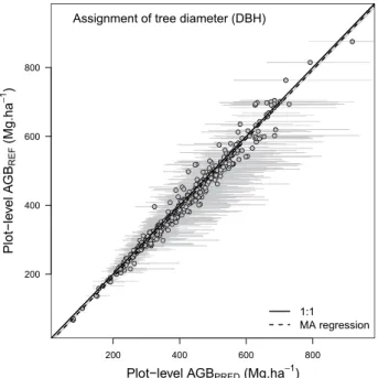
Using the generic exponential PDF, the assignment of continuous diameters from discrete diameter classes propagated a relatively moderate uncertainty to plot-level AGB that varied with the position of the open diameter class. For instance, the average uncertainty was 0.4% (0.2–0.8) and 4.6% (1.4–12.0) when tree diameters above 200 cm and 120 cm were pooled in a single ‘open class’ (Fig. 6a), respectively. The tree diameter assignment function did not propagate a systematic error across the range of plots’ AGB (slope of the MA regression: 1.00 [0.98–1.01], Fig. 7)Validation of the small tree simulation function (specific function 2).
The small tree simulation procedure was evaluated using the scientific dataset by removing information on small trees so as to matchFig. 6 Validation of the AGB computation scheme with scientific inventory data. (a) Mean ± 95% confidence interval of plot-level coefficient of variation (CV) on AGB estimation when propagating a single (WD: wood density, H: height-diameter model, AGB: biomass model, DBH: continuous tree diameter assignment function, Nexp: small tree simulation function, AGBcor: biomass correction model for trees in 10–20 cm DBH class)
or several error sources combined. For the assignment of tree DBH, we simulated two contrasted scenarios corresponding to a diameter threshold for the open diameter class of 200 cm (open circles) and 120 cm (full circles). For the simulation of small trees, we simulated the two most contrasted scenarios found in commercial data, namely (i) a partial inventory on diameter class 10-20 cm only (over 25% of plot area, open circles) vs (ii) a partial inventory on diameter classes 10–20, 20–30 and 30–40 cm (over 12.5, 12.5 and 25% of plot area, respectively, full circles). We finally propagated all error sources (noted ALL) following the best (open circles) and worst (full circles) case scenarios. In the latter case, trees in the 10-20 cm diameter class were completely removed and the AGB correction model for this class was used. (b) Plot-level AGB estimates of scientific reference data against predicted AGB based on degraded data so as to match the worst-case scenario (noted ALL in the left panel) found in commercial inventories. Grey dots and bars represent the mean and 95% confidence interval of plots biomass, respectively.
varying sampling scenarios observed in commercial data. Figure 8 shows the results of the procedure (AGBPRED
based on expanded small tree abundance, NEXP) against reference AGB (i.e. computed on full scientific data)
when simulating the lightest sampling of small trees found in forest management inventory data (or ‘worst-case scenario’, i.e. c. 12.5%, 12.5% and 25% sampling for diameter classes 10–20 cm, 20–30 cm and 30–40 cm, respec-tively). While within-plot AGB variation induced by the sole small tree simulation function was high in this extreme sampling scenario (with an average plot CV of 7.7% (95% CI: 3.4–13.9), Fig. 6a), it led to a very slight estimation bias across plots (slope of the MA regression: 0.97 [0.95–0.99], Fig. 8).
Fig. 7 Results of the tree diameter assignment function. AGBREF corresponds to an average of 1000 plots
AGB simulations while propagating wood density, height-diameter and allometric model errors. In AGBPRED
(mean ± SD), the error associated with the tree diameter assignment function is also propagated. Grey dots and bars represent the mean and 95% confidence interval of plots biomass, respectively.
Fig. 8 Results of the small tree simulation function. AGBREF corresponds to an average of 1000 plots AGB
simulations while propagating wood density, height-diameter and allometric model errors. In AGBPRED
(mean ± SD), the error associated with the small tree simulation function is also propagated. Grey dots and bars represent the mean and 95% confidence interval of plots biomass, respectively.
Validation of the biomass correction model for trees in diameter class 10–20 cm (specific
func-tion 3).
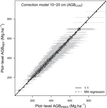
We removed trees in the 10-20 cm diameter class from scientific inventories and computed plot AGB using the AGB10-20 model for that class. The sole biomass correction model propagated an uncertainty of 6.4% onplot AGB estimates (95% CI: 3.3–11.5; Fig. 6a) and led to accurate AGB estimates across plots (slope of the MA regression: 0.99 [0.99–1.00], Fig. 9).
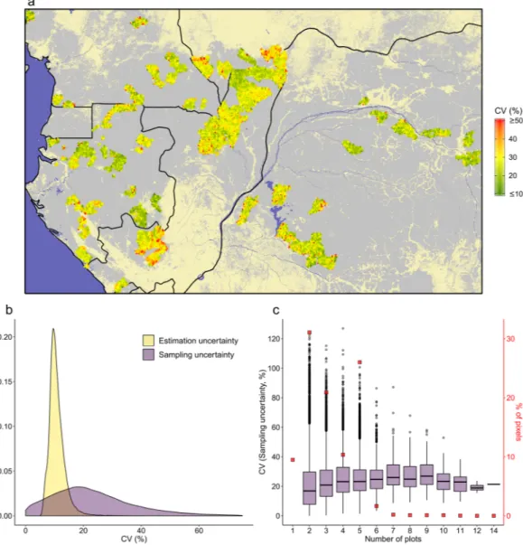
assessment of pixel-level uncertainty.
Once aggregated into 1-km pixels, the total uncertainty (CV) on pixel AGB estimates was 26.3% on average and mostly comprised between 9.3% (quantile 2.5) and 61.1% (quan-tile 97.5). The spatial distribution of pixels total CV shows some clusters of pixels with lower uncertainty level (Fig. 10a), generally corresponding to high-biomass areas (as illustrated in Fig. 1). Pixel total CV was largely domi-nated by the sampling uncertainty (i.e. the inter-plot variance within pixels, Fig. 10b). When considered separately, the sampling and estimation (i.e. the mean intra-plot variance within pixels) uncertainties represented a mean CV (±sd) of 23.5% ± 14.9% and 11.8% ± 2.9%, respectively. While the sampling uncertainty did not depend strongly to the number of plots per pixel (Fig. 10c), the associated confidence interval on pixel mean AGB decreased with the squared root of the number of plots, from c. 26.7% to 20.7% and 14.9% for 3, 6 and 10 plots, respectively.Usage Notes
Given its size and regional coverage, this dataset should be particularly useful to the community of remote-sensing scientists working on tropical forest biomass. Developing, validating or comparing large-scale remote sensing models of tropical forest biomass is made difficult by the absence of standard, readily available large scale ref-erence datasetseg.36. While the Global Ecosystem Dynamics Investigation (GEDI) sensor onboard the
interna-tional space station will provide billions of discrete biomass estimations across the globe for the early 2020s37, the
only reference data currently available for the first decade of the century are derived from the Geoscience Laser Altimeter System (GLAS). Biomass estimations computed from the CoFor dataset constitute the unique alterna-tive to those from GLAS for large-scale remote-sensing applications in the central African region for this period. This dataset could also be used to re-calibrate existing global biomass maps, which has proven useful to increase the precision of mean biomass estimations over regions or forest types of interest using design-based inference38.
In that, the potential of these data to improve the precision of carbon stocks or carbon emission factors used in national or jurisdictional REDD + projects in central Africa could be investigated. These data are also relevant to study the sensitivity of forest carbon to environmental conditions, which could provide insights into the poten-tial response of forest carbon to climate change, a major source of uncertainty in current global climate models. By providing a decomposition of pixels’ forest biomass into its structural (number of trees, mean tree diameter) and compositional (i.e. mean wood density) characteristics at plot-level, we also expect these data to be useful to study local and regional variation patterns. Wood density for instance cannot be detected and mapped over large scales with current remote sensing data types. The data released here could thus be used, just like pixels biomass, as a calibration/validation set for wood density spatial models based on environmental data, or to derive ecosystem-levels means.
Fig. 9 Results of the AGB correction model for trees in diameter class 10–20 cm. AGBREF corresponds to an
average of 1000 plots AGB simulations while propagating wood density, height-diameter and allometric model errors. In AGBPRED (mean ± SD), the error associated with the AGB correction model for trees in diameter
class 10–20 cm is also propagated. Grey dots and bars represent the mean and 95% confidence interval of plots biomass, respectively.
It should be noted that forest biomass in CoFor sample plots is based on stem diameter distribution and spe-cies averaged tree wood densities, while tree heights have been predicted from a regional allometry model. Tree diameter-height allometry varies locally39, and the regional model we used is known to produce biased estimates
at some sites40. This error will thus propagate to plot biomass estimations. A similar pattern of opposite errors can
be expected from GLAS-derived biomass estimations, which are based on height measurements with no infor-mation on the underlying stem diameters.
Code availability
All analyses were performed in R (v.3.6.2). The BIOMASS R-package is an open source library available from the CRAN R repository. Codes associated to specific functions are available upon request.
Received: 18 March 2020; Accepted: 8 June 2020; Published: xx xx xxxx
References
1. Parde, J. Forest biomass. In Forestry Abstracts vol. 41 343–362 (Commonwealth Agricultural Bureaux, 1980). 2. Mitchard, E. T. A. The tropical forest carbon cycle and climate change. Nature 559, 527–534 (2018).
3. Herold, M. et al. The role and need for space-based forest biomass-related measurements in environmental management and policy.
Surv. Geophys. 40, 757–778 (2019).
Fig. 10 Uncertainties on pixel-level AGB estimates. (a) Total uncertainty on 1-km pixels AGB estimates (reported as a coefficient of variation, CV, in %), aggregated into 5-km pixels (for visual purpose), is depicted in a green-to-red color gradient and underlaid by the spatial distribution of moist forests21 (grey) and
countries borders (black). (b) Frequency distribution of estimation and sampling uncertainties across pixels. (c) Distribution of sampling uncertainty by categories of pixels. Categories reflect the number of forest management plots available by pixel to compute pixel’s AGB. The proportion of each category in the CoFor dataset (in %) is represented with red square symbols.
4. Pan, Y. et al. A large and persistent carbon sink in the world’s forests. Science 333, 988–993 (2011).
5. Mitchard, E. T. et al. Uncertainty in the spatial distribution of tropical forest biomass: a comparison of pan-tropical maps. Carbon
Balance Manag 8, 10 (2013).
6. Houghton, R. A. et al. Annual fluxes of carbon from deforestation and regrowth in the Brazilian Amazon. Nature 403, 301–304 (2000).
7. Baccini, A. et al. Estimated carbon dioxide emissions from tropical deforestation improved by carbon-density maps. Nat. Clim.
Change 2, 182–185 (2012).
8. Song, X.-P. et al. Global land change from 1982 to 2016. Nature 560, 639–643 (2018).
9. Maxwell, S. L. et al. Degradation and forgone removals increase the carbon impact of intact forest loss by 626%. Sci. Adv. 5, eaax2546 (2019).
10. Andrade, R. de O. Alarming surge in Amazon fires prompts global outcry. Nature, https://doi.org/10.1038/d41586-019-02537-0. (2019)
11. Aragão, L. E. O. C. et al. 21st Century drought-related fires counteract the decline of Amazon deforestation carbon emissions. Nat.
Commun. 9, 536 (2018).
12. McRoberts, R. E., Tomppo, E. O. & Næsset, E. Advances and emerging issues in national forest inventories. Scand. J. For. Res 25, 368–381 (2010).
13. Avitabile, V. & Camia, A. An assessment of forest biomass maps in Europe using harmonized national statistics and inventory plots.
For. Ecol. Manag 409, 489–498 (2018).
14. Vidal, C., Bélouard, T., Hervé, J.-C., Robert, N. & Wolsack, J. A new flexible forest inventory in France. In Proceedings of the seventh
annual forest inventory and analysis symposium; October 3-6, 2005; Portland, ME. Gen. Tech. Rep. WO-77 vol. 77 67–73 (Washington,
DC: US Department of Agriculture, Forest Service, 2007).
15. Manuel de terrain de l’Inventaire Forestier National de la République Démocratique du Congo. vol. Version 1.0. (Ministère de l’Environnement et Développement Durable, 2017).
16. Kandler, G. The design of the second German national forest inventory. In Proceedings of the eighth annual forest inventory and
analysis symposium; 2006 October 16-19; Monterey, CA. Gen. Tech. Report WO-79 vol. 79 19–24 (Washington, DC: US Department
of Agriculture, Forest Service, 2009).
17. Duncanson, L. et al. The importance of consistent global forest aboveground biomass product validation. Surv. Geophys. 40, 979–999 (2019).
18. Chave, J. et al. Ground data are essential for biomass remote sensing missions. Surv. Geophys. 40, 863–880 (2019).
19. Wasseige, C. DE et al. Les Forêts du Bassin du Congo: etat des Forêts 2008. (Office des publications de l’Union européenne, 2009). 20. Rapport stratégique régional. Développement intègre et durable de la filière bois dans le bassin du Congo: opportunités, défis et
recommandations opérationnelles. (Banque Africaine de Développement, 2019).
21. CCI, ESA. New release of 300 m global land cover and 150 m water products (v.1.6.1) and new version of the User Tool (3.10) for
download. (ESA CCI Land cover website, 2016).
22. Réjou-Méchain, M. et al. Detecting large-scale diversity patterns in tropical trees: Can we trust commercial forest inventories? For.
Ecol. Manag 261, 187–194 (2011).
23. Ploton, P. Africadiv extract. figshare https://doi.org/10.6084/m9.figshare.11865540 (2020).
24. Anderson‐Teixeira, K. J. et al. CTFS-ForestGEO: a worldwide network monitoring forests in an era of global change. Glob. Change
Biol. 21, 528–549 (2015).
25. Bastin, J.-F. et al. Aboveground biomass mapping of African forest mosaics using canopy texture analysis: toward a regional approach. Ecol. Appl. 24, 1984–2001 (2014).
26. Phillips, O. L., Baker, T., Feldspauch, T. & Brienen, R. J. W. Field manual for plot establishment and remeasurement (RAINFOR).
Amaz. For. Inventory Netw. Sixth Framew. Programme 2002–2006 (2002).
27. Réjou‐Méchain, M., Tanguy, A., Piponiot, C., Chave, J. & Hérault, B. biomass: an r package for estimating above-ground biomass and its uncertainty in tropical forests. Methods Ecol. Evol 8, 1163–1167 (2017).
28. Chave, J. et al. Improved allometric models to estimate the aboveground biomass of tropical trees. Glob. Change Biol. 20, 3177–3190 (2014).
29. Zanne, A. E. et al. Data from: Towards a worldwide wood economics spectrum. Dryad, https://doi.org/10.5061/dryad.234 (2009). 30. Feldpausch, T. R. et al. Tree height integrated into pan-tropical forest biomass estimates. Biogeosciences 9, 3381–3403 (2012). 31. Schepaschenko, D. et al. The Forest Observation System, building a global reference dataset for remote sensing of forest biomass. Sci.
Data 6, 1–11 (2019).
32. VanDerWal, J. et al. Package ‘SDMTools’. R Package (2014).
33. Devroye, L. Sample-based non-uniform random variate generation. In Proceedings of the 18th conference on Winter simulation 260–265 (ACM, 1986).
34. Ploton, P. et al. A 1-km resolution dataset of African humid tropical forests aboveground biomass derived from management inventories. figshare https://doi.org/10.6084/m9.figshare.11865450 (2020).
35. Ploton, P. et al. Aggregated CoFor forest management inventories. figshare https://doi.org/10.6084/m9.figshare.11993541 (2020). 36. Rodríguez-Fernández, N. J. et al. An evaluation of SMOS L-band vegetation optical depth (L-VOD) data sets: high sensitivity of
L-VOD to above-ground biomass in Africa. Biogeosciences 15, 4627–4645 (2018).
37. Dubayah, R. et al. The Global Ecosystem Dynamics Investigation: High-resolution laser ranging of the Earth’s forests and topography. Sci. Remote Sens 1, 100002 (2020).
38. Næsset, E. et al. Use of local and global maps of forest canopy height and aboveground biomass to enhance local estimates of biomass in miombo woodlands in Tanzania. Int. J. Appl. Earth Obs. Geoinformation 89, 102109 (2020).
39. Beirne, C. et al. Landscape‐level validation of allometric relationships for carbon stock estimation reveals bias driven by soil type.
Ecol. Appl. 29, e01987 (2019).
40. Kearsley, E. et al. Conventional tree height–diameter relationships significantly overestimate aboveground carbon stocks in the Central Congo Basin. Nat. Commun. 4, 1–8 (2013).
acknowledgements
P.P. was supported by a 3DForMod post-doctoral grant. The 3DForMod project was funded in the frame of the ERA-NET FACCE ERA-GAS (ANR-17-EGAS-0002-01), which has received funding from the European Union’s Horizon 2020 research and innovation program under grant agreement No 696356. We thank the logging companies that provided access for research purposes, albeit restricted, to the inventory data of their concessions, as well as the consulting firms FRMi and TEREA that acted as intermediaries. Scientific plots establishment benefited from IFS grant number D/5621-1, European Union Climate KIC grant Agreement EIT/CLIMATE KIC/SGA2016/1 and grant N° TF010038 from the Global Environment Facility administered by the World Bank and implemented by the COMIFAC. We would like to thank Shell Gabon and the Smithsonian Conservation Biology Institute for funding the collection of the Rabi data in Gabon (contribution No 197 of the Gabon Biodiversity Program).
author contributions
P.P., F.M., R.P. and S.G.F. conceived the study, analyzed the data and led the writing of the paper. S.G.F., N.Bay., B.D., J.L.D, F.B. and G.C. collated management inventory data. A.A., J.F.B., P.B., G.C., V.D., N.G.K., D.K., H.M., L.M., B.S., N.T., D.T. and D.Z. participated to the collection of scientific inventory data. M.R.M., N. Bar., V.D. and V.R. commented on analyses and provided critical inputs for the writing of the paper. All authors read and approved the final manuscript.
Competing interests
The authors declare no competing interests.
additional information
Supplementary information is available for this paper at https://doi.org/10.1038/s41597-020-0561-0.
Correspondence and requests for materials should be addressed to P.P.
Reprints and permissions information is available at www.nature.com/reprints.
Publisher’s note Springer Nature remains neutral with regard to jurisdictional claims in published maps and
institutional affiliations.
Open Access This article is licensed under a Creative Commons Attribution 4.0 International
License, which permits use, sharing, adaptation, distribution and reproduction in any medium or format, as long as you give appropriate credit to the original author(s) and the source, provide a link to the Cre-ative Commons license, and indicate if changes were made. The images or other third party material in this article are included in the article’s Creative Commons license, unless indicated otherwise in a credit line to the material. If material is not included in the article’s Creative Commons license and your intended use is not per-mitted by statutory regulation or exceeds the perper-mitted use, you will need to obtain permission directly from the copyright holder. To view a copy of this license, visit http://creativecommons.org/licenses/by/4.0/.
The Creative Commons Public Domain Dedication waiver http://creativecommons.org/publicdomain/zero/1.0/
applies to the metadata files associated with this article. © The Author(s) 2020