Digitized
by
the
Internet
Archive
in
2011
with
funding
from
Boston
Library
Consortium
IVIember
Libraries
working paper
department
of
economics
THE AGGREGATE MATCHING FUNCTION
Olivier Jean Blanchard
Peter Diamond No. 538 October 1989
massachusetts
institute
of
technology
50 memorial
drive
Cambridge, mass.
02139
THE AGGREGATE MATCHING FUNCTION
Olivier Jean Blanchard
Peter Diamond
The Aggregate Matching Function
Olivier Jean Blanchard and Peter Diamond
Abstract
We present a picture of the labor market, one with large flows of jobs and workers,
and matching. We develop a consistent approach to the interaction among those flows
and the stocks of unemployed workers and vacant jobs, and to the determination of
wages. We estimate the matching function, using both aggregate data and data from
manufacturing and find evidence of a stable matching process in the data. We examine
the joint movements in unemployment, vacancies and wages -the Beveridge and Phillips
curve relations- in the light of our model. We conclude that aggregate activity shocks
September 21, 1989
The Aggregate Matching Function
Olivier Jean Blanchard and Peter Diamond
MIT. This paper is in part an alternative presentation of the material in our
1989 paper. In addition, we report on additional findings on the aggregate matching
function and start looking, theoretically and empirically, at wage determination and
the relation between the Phillips and Beveridge Curves. Ve thank the NSF for financial
assistance and DRI for access to their data base. we thank Hugh Courtney and Juan
Jimeno for excellent research assistance, John Abowd and Arnold Zellner for their gross
flow data, Kathy Abraham for help with the vacancy data, George Ak,erlof, Nils
Gottfries, Bob Hall, Jerry Hausman, Larry Katz, Chris Pissarides, Bob Solow, Larry
Bob Solow has written: "Any time seems to be the right time for reflections on the
Phillips curve"(1976) . And since his 1960 paper with Paul Sarauelson, he has reflected
many times.
Their joint paper is widely known for having drawn the first American Phillips
curve. In fact, having drawn it, Samuelson and Solow quickly put distance between
themselves and the curve. Having duly noted the empirical fit, they pointed out that
the Phillips curve had disappeared during the Depression, and suggested that persistent
high unemployment could well reduce labor mobility and increase structural
unemployment. They expressed skepticism as to the long run trade off, writing, "it
would be wrong, though, to think that our figure 2 menu that relates obtainable price
and unemployment behavior will maintain the same shape in the longer run". They argued
that imperfect competition was the right setting for studying cost push inflation.
They em.phasized that many factors were at work in the labor market including labor
reallocation, labor mobility, collective bargaining; thus no simple or single
explanation was likely to account for the relation between wages and unemployment.
Many of Solow' s later papers were further explorations of those early themes. His
1954 Vicksell lectures developed the view of the labor market as a market with constant
reallocation of labor and addressed the question of how much of unemployment was due to
low demand and how much to structural factors. To do so, he brought to the scene both
the Phillips curve and the Beveridge curve, a strategy we shall pursue below. In his
might be jolted out of an underemployment equilibrium". Solow's more recent work has
returned to the relation between collective bargaining and unemployment. In a field
where fashion rules, the papers read as well or better today than when they were
written. This is because they combine four traits -an eye on the facts, an eclectic
view of the large number of complications which are relevant for the short run behavior
of the economy, an awareness of the implications of neoclassical theory, and an
unwillingness to give neoclassical implications more than their due.
We are both students of Solow, one of Solow the growth theorist, the other of Solow
the macroeconomist. One of us came to study labor markets as a result of the internal
logic of a research program based on the idea that decentralized markets work very
differently from models designed for centralized markets. The other was motivated by
the recent European experience, and the potential role of collective bargaining in
explaining the persistence of unemployment. Our collaboration on this paper was begun
two years ago to take up two challenges. The first was whether, as a team, we could
emulate the back and forth between theory and empirical work which Solow does so well
alone. The second was to find a framework for thinking about collective bargaining in
labor markets characterized by large flows and constant reallocation of labor across
jobs. V,'e are not yet where we want to go. Put more bluntly, we have captured the
large flows but not yet introduced collective bargaining. Nevertheless, we think we
have made progress; this paper is a progress report.
Our basic theme is that the labor market is a market with large flows of workers,
and simultaneously large rates of job creation and destruction. Evidence on the large
flows of workers in the US comes from the monthly household sur^'ey. While the raw data
removed. The series as adjusted by Abowd and Zellner imply that, each month, roughly
7% of the labor force moves in or out of employment. While this could be consistent
with workers reallocating themselves across a given set of jobs, recent evidence by
Davis and Haltiwanger shows this not to be the case. Looking at a large number of
establishments, they compute a measure of job turnover, defined as the sum of
employment increases in new or expanding establishments, and emplo}Tiient decreases in
shrinking or dying establishments. They find that in manufacturing, over the period
1979-1983, a period of shrinking employment, job turnover was of the order of 10% per
quarter
.
Thus, at any point in time, many firms are looking for workers, many workers are
looking for jobs. How many hires result from a given number of vacancies and workers
depends on the geography of job destruction and job creation, on skill differences
between workers and jobs, on how eagerly workers and firms are looking for each other
and so on. In the same spirit as Solow used an aggregate production function,
bypassing complex issues of aggregation to get to the basic issues of growth and
productivity, we start our paper by estimating an aggregate matching function, giving
the flow of hires as a function of the stocks of vacancies and unemployment . We
estimate this function for the US for the period 1968-1981 -the only period for which
the required data are available. We find a stable, Cobb-Douglas matching function with
a declining time trend, equal weight on vacancies and unemployment and constant or
mildly increasing returns to scale. Thus very much like the production function, the
abstraction turns out to be both conceptually helpful and empirically relevant. We
2
then make two attempts at estimating disaggregated matching functions. Both are
hampered by problems of data quality, but both turn out nevertheless to give
interesting results. The first looks at matching in manufacturing. For a brief period
of time, 1969-1973, the BLS collected monthly vacancy statistics for manufacturing;
this allows estimation of a matching function for that period. Much like the
aggrregate matching function, the matching function for manufacturing exhibits roughly
equal weights on vacancies and unemployment, and mildly increasing returns. The second
attempt is motivated by the fact that close to 40% of new hires are of people
officially classified as "out of the labor force". Thus, we look separately at hires
from the unemployment pool and hires from "out of the labor force". The two hires
series are available separately, and BLS provides a series for workers classified as
"out of the labor force but wanting a job", which can be taken as a proxy for the
relevant pool of people "out of the labor force" . The data show sharp differences
between the two groups, differences which are consistent with differences in either the
variation of search intensity through time, and in the way employers view and choose
between the two groups.
Using the aggregate matching function, we build a simple model of the labor market
which focuses on the flows in Sections 2 and 3. It has two basic ingredients. The
first is that it takes time to reallocate, to match workers and jobs; this is captured
by the matching function. The second is the assumption that there is unceasing job
destruction and job creation, continual layoffs and posting of vacancies. Wages are
assumed to divide the surplus from a match between a worker and a job; a natural
assumption is that of Nash bargaining. Thus, there is no tight connection between wages
and employment. At any point in time, a change in the wage -coming say from changes in
affect the profitability of jobs, the supply of jobs and the level of employment. This
lack of an allocational role for the wage in the short run is surely too strong;
however it is likely to be a better approximation to the role of wages than the other
extreme, that employment depends on the wage even in the very short run.
The model makes clear predictions about how different shocks affect unemployment,
vacancies and wages. Contractions in aggregate activity increase unemployment and
decrease vacancies, both putting downward pressure on wages. In contrast, periods of
intense reallocation increase both unemployment and vacancies but may be associated
with little or no pressure on wages. This suggests that an empirical examination of
the joint behavior of the Phillips and Beveridge curves through the lenses of the model
can tell us a lot about the sources of the shocks affecting an economy. Put too
strongly, the model allows us to look, in an integrated fashion, at the Beveridge curve
and the Phillips curve. The statement is too strong because, at this stage, we stay
away from formalizing nominal rigidities, although we suggest how they can be naturally
introduced. We have started following this lead and, in Section 4, report on some of
our progress for the postwar US. We have worked hard on the Beveridge curve, but just
peeked at the Phillips curve. Our conclusions at this stage are that, in the post war
US, major movements in unemployment have been mostly the result of changes in aggregate
activity, not of changes in the intensity or the effectiveness of the reallocation
process. Reallocation changes appear however to have played a more important role at
lower frequencies. These conclusions probably sound more authoritative than is
warranted: our preliminary examination of the Phillips curve yields a number of puzzles
1. The Aggregate Matching Function
If the right picture of the labor market has constant churning of workers and jobs,
the matching process is at the center of the picture. Thinking in terms of an
aggregate matching function is an attractive way of thinking about the dynamics of
hiring and employment. It is more appealing than postulating a stock adjustment
equation for employment. It is also more appealing than equating employment with labor
demand, another standard alternative. If the speed of filling vacancies did not depend
on labor market conditions, we would find no role for unemployment in the matching
process. As we shall see below, this is not the case.
Estimation of an aggregate matching function can also shed light on the role of
different classes of workers (short term-long term, skilled-unskilled, in or out of the
labor force) in the matching process. Micro studies are no substitute for that
information. For example, cross section results on the importance of unemployment
compensation for the likelihood of finding a job do not translate directly into
implications for aggregate unemployment since less availability by some workers will
raise the probability of job finding by others.
Why might even a believer in the importance of labor market flows object to giving a
central role to the matching function? We have heard two objections. The first is
that the concept of a vacancy is much vaguer than the concept of an unemployed worker,
making it unlikely that vacancies are a useful concept for organizing empirical work.
We feel that the concepts of unemployed workers and vacancies both represent an attempt
to substitute a scalar variable (the number available) for a schedule of availability
as a function of the attractiveness of opportunities. In both cases, whether those
empirical success when they are used. And, as we shall see, both series appear to be
successful in that regard. A separate but related issue is that there does not exist a
vacancy series for the US -or any other country we know of- constructed with the care
and coverage of the unemployment series. In the US, the substitute we have is the
Conference Board's Help Wanted Index which has been adjusted by Katharine Abraham to
better approximate vacancies. Again, the adequacy of that proxy must be judged in the
end by how it performs in estimation. For 1969 to 1973, we do have a vacancy series
for manufacturing. We also report estimates using that data.
The second objection is of a different nature. It is that vacancies are only an
intermediate variable, and that one must explain how new vacancies evolve over time.
It is indeed true that the matching function is only part of the story; any complete
story must account for job creation and job destruction and their determinants. It is
nevertheless an essential part of the story. Again, the parallel with the aggregate
production function is an obvious one.
In thinking about matches, we envision each worker and firm as engaged in a time
consuming (stochastic) process of waiting for and looking for an appropriate match. We
formalize the matching process by an aggregate function which gives new hires, h, as a
function of unemployment and vacancies:
(1) h = Q m(U,V)
where a is a scale parameter, and m^, my > 0, m(0,V)=m(U, 0)=0
.
This matching function recognizes that the large labor market flows in the US generate
delays in the finding of both jobs and workers. From, a macroeconomic point of view,
i.e., leaving aside the heterogeneity of individual workers or vacancies, the process
the average duration of vacancies does not exceed a month. But the process is simply
not infinitely efficient and the speeds of job finding and job filling vary noticeably
over the cycle. Changes in the parameter a are intended to capture changes in
geographic or skill distributions of jobs and workers, -what is sometimes called
mismatch- as well as differences in search and match acceptance behavior. In
estimation below, a is formalized as a deterministic time trend.
Given the size of the flows relative to the stocks, it is essential to estimate the
matching function using the highest frequency data available, which here means monthly
data. None of the series needed to estimate the matching function is directly
available and we construct them as follows (Specific sources and details of
construction are given in our BPEA paper)
.
We construct new hires as the sum of the flows into employment from unemployment and
from out of the labor force (taken from the CPS gross flows data as adjusted by Abowd
and Zellner (1985) and deseasonalized using frequency domain filtering) , to which we
add the flow from employment to employment (estimated as 0.4 times the manufacturing
quit rate times employment; for a discussion of employment to employment quits see
Akerlof, Rose, and Yellen (1988)), and from which we subtract the flow of workers who
are recalled rather than newly hired (estimated as 1.5 times manufacturing recalls).
The resulting new hires series is plotted in figure 1, along with our measures of
unemployment and vacancies described below. One obvious characteristic of the series
is its large high frequency movements, which in turn come from the movements in the CPS
gross flow series. We believe that these movements come largely from sampling and
classification error: the Abowd-Zellner adjustment removes the mean error but not its
random component. If this is the case, the series can still be used as a left hand
|NJ UJ LH cn CD CD CO CO CO CO
O
CO C_ -<1 CO -0 ro CO CO CO --J CO cn LD^
-^<
-n ZDm
CD—
c_ z: =DO
CD CD LD CO CO CO CO CD CO CO CO10
The composition of the gross flow into employment shows clearly that the relevant
pool of workers includes more than just the unemployed. We estimate that on average
^^5% of new hires come from unemployment, A0% from out of the labor force and 15%
directly from employment. By using unemployment in most of what follows, we implicitly
assume that the relevant pool is proportional to the pool of unemployed workers. We
take the pool of unemployment to equal to the total number of unemployed workers minus
those workers classified as "job losers on layoff", workers who consider themselves as
having a job. We explore alternative definitions of the pool below.
For the aggregate vacancy series we use the help-wanted series constructed by the
Conference Board, and adjust it following Abraham (1983, 1987). We adjust the level of
the series so that its mean is similar to the mean reported vacancy rate for the
periods of time for which such a rate is available (Abraham 1983, table 3). This
yields a mean vacancy rate of 2.2% for the period 68:1 to 81:12, the period for which
all the data we use are available. The mean of the unemployment rate as defined is
4.8% for this period.
The aggregate matching function: basic specifications
Our basic specification gives new hires as a Cobb Douglas function of vacancies and
unemployment, with all variables defined as above:
ln(Hj.) - a + b time + c ln(Vj..^) + d ln(U^.]_) + e^
There is no clean way of handling timing. First, reality is in continuous time and
ve have discrete time data. With the mean duration of vacancies under a month, a
literal interpretation of an equation such as the one above would make no sense as the
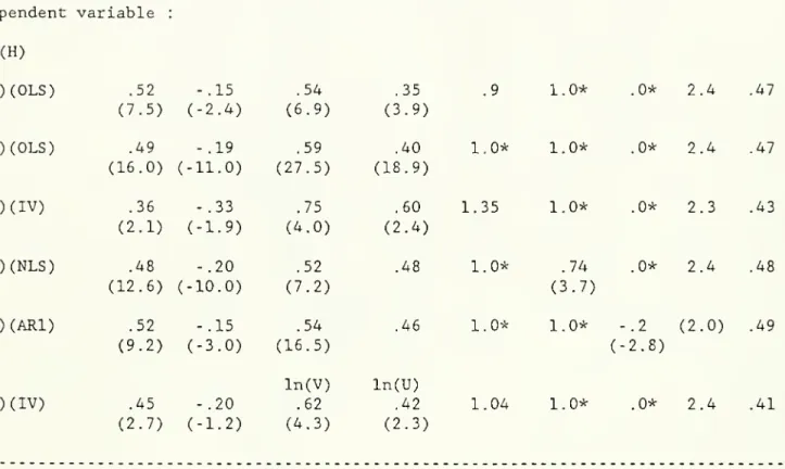
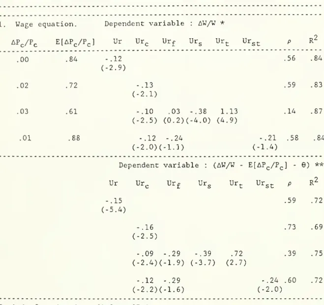
Table 1. The aggregate matching function
Basic specifications
Independent variables : coefficients on :
time (xlO"2)
constant time ln(V(-l)) ln(U(-l)) RTS elasticity p DW R^
•2< Dependent variable : ln(H) (1)(0LS) .52 -.15 .54 .35 .9 1.0* .0* 2.4 .47 (7.5) (-2.4) (6.9) (3.9) (2)(0LS) .49 -.19 .59 .40 1.0* 1.0* .0* 2.4 .47 (16.0) (-11.0) (27.5) (18.9) (3)(IV) .36 -.33 .75 .60 1.35 1.0* .0* 2.3 .43 (2.1) (-1.9) (4.0) (2.4) (4)(NLS) .48 -.20 .52 .48 1.0* .74 .0* 2.4 .48 (12.6) (-10.0) (7.2) (3.7) (5)(AR1) .52 -.15 .54 .46 1.0* 1.0* -.2 (2.0) .49 (9.2) (-3.0) (16.5) (-2.8) ln(V) ln(U) (6)(IV) .45 -.20 .62 .42 1.04 1.0* .0* 2.4 .41 (2.7) (-1.2) (4.3) (2.3) Period of estimation : 68:2 to 81:12 t statistics in parentheses
Instruments for (3) : In(IP), lagged two to four times ; IP : industrial production
Instruments for (6) : ln(V) , ln(U) lagged one to three times
11
time. Insofar as the discrete time specification works empirically, it relies on the
smoothness of the continuous time pattern of vacancies. Second, while one would want
to regress new hires during the month on the two stocks at the same time of the month,
the data do not come in that form. Some of our data are point in time, some integrals
of stocks (for vacancies) or flows (for hires) over time. Our specification is a
compromise. Ue also present the results of estimation with current values of V and U,
instrumented by their lagged values.
The results are presented in table 1. The first regression estimates the equation
as specified above. The second imposes constant returns, i.e., c+d=l. Both use OLS
.
However, if the disturbance term to the hiring function includes a serially correlated
component, OLS estimation may lead to a downward bias in the estimated coefficients on
unemployment and vacancies: a positive disturbance to hiring leads, ceteris paribus, to
a decrease in unemployment and vacancies. Thus, the third regression estimates the
equation using industrial production, lagged two to five times as an instrument: to the
extent that firms can vary hours to compensate for disturbances in hiring, industrial
production is likely to be affected less by disturbances to the matching function than
are either unemployment or vacancies. Thus, the use of industrial production surely
removes some, although perhaps not all, of the bias. The fourth regression allows for
the elasticity of substitution between V and U to differ from one, by estimating a CES
instead of a Cobb Douglas specification. The fifth allows for first order serial
correlation in the disturbance term. The sixth uses current values of V and U,
instrumented by their own lagged values. There is no evidence in favor of a more
complex lag structure.
The results are clear cut and vary little over specifications. The hiring process
12
scale, unit elasticity of substitution, and relative weights of .6 and .4 on vacancies
and unemployment. Returns to scale, are slightly less than 1.0 when estimated by OLS
,
but increase to 1.35 when lagged industrial production is used as an instrument
(lagging industrial production further does not increase the estimated degree of
returns to scale); the elasticity of substitution, when estimated, is equal to .74, not
significantly different from one. All specifications yield a trend decline in hires
given unemployment and vacancies; using the first regression, the trend decline is of
roughly 25% over the sample period. Using the third regression, the decline is roughly
40% over the sample period. With a specification that does not distinguish short from
long run returns to scale, a greater estimate of returns to scale will tend to go with
a more rapidly declining trend.
The result that both unemployment and vacancies matter implies that the rate of
hiring is determined by both sides of the labor market, not only by demand. Put
another way, the average duration of vacancies varies with the vacancy-unemployment
ratio. The adjusted unemployment-vacancy ratio varies between 5.0 and 0.9 over this
period. Using regression (2), we estimate that the average duration of vacancies is
equal to 2 weeks, when the ratio is equal to 5; when the ratio equals .9, the average
duration of vacancies increases to 4 weeks . Just as with unemploj-ment, the average
duration also hides differences in durations across vacancies; a 1954 Rochester study
(Myers and Creamer 1967) found that, while the median duration was 4 weeks, more than
3
One can obviously compute the average duration of unemployment as well. The two
corresponding numbers are 2.3 and .8 months. But as unemployment proxies for a larger
13
A0% of vacancies had durations in excess of 6 weeks and 20% had durations in excess of
12 weeks .
The presence of a negative trend during the sample suggests a potential proximate
source for the shift in the Beveridge curve, an issue to which we shall briefly return.
Where this trend comes from,however. we do not investigate further.
Recent theoretical developments have argued for the plausibility and potential
importance for macroeconomics of increasing returns in matching . Plausibility of
increasing returns comes from the idea that active, thick, markets may lead to easier
matching. The evidence suggests increasing, but not strongly increasing returns. Some
downward bias may remain in this estimate, so that proponents of strongly increasing
returns in the labor market may still have hope. Whatever the findings for the labor
market, the different structure of the goods market leaves open the possibility of
strong increasing returns to matching in the goods market.
Finally, we find no evidence of further non-linearities; we have explored the idea
that, as unemployment increases, firms find workers as easily as they want, so that
further increases in the unemplojTiient rate, given vacancies, do not increase hiring.
When we allow for additional non-linear term.s in unemployment, or split the sample
according to the value of the unemployment -vacancy ratio, we find no evidence of such
an effect.
If the arrival rate of workers were constant, a median duration of vacancies of 4
weeks would imply a mean of 5.7 weeks ; 35% of vacancies would last more than 5 weeks.
^ See Diamond (1982)
14
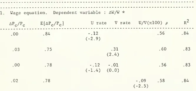
The matching function for manufacturinp:. 1969-73
The necessity of constructing the time series used in the empirical work reported in
table 1 makes it appealing to explore the matching function for manufacturing where the
data needed were collected directly, if only briefly. New hires in manufacturing were
collected on a monthly basis until 1981, and, in a four year experiment, from 1969 to
1973, data on vacancies at the end of the month were also collected. In table 2, we
report some results using these alternative series. We use the same unemployment
variable as earlier . Since the time series is so short we omit the time trend. The
first regression reports the results of OLS estimation, the second of IV estimation
using lagged industrial production as an instrument. They give similar results, and
results consistent with those of table 1. Both vacancies and unemployment are
significant, with approximately equal coefficients. This result, which again implies
that manufacturing vacancies are harder to fill when unemplo^Tnent is low, suggests that
the image of manufacturing as a sector where workers queue for jobs, and firms just
need to choose from a pool of waiting workers -as in efficiency wage models- is not
quite correct. The average duration of a vacancy is lower for manufacturing than for
the economy as a whole, roughly 10 days on average for the period we consider ; but the
While there exists a series giving the number of unemployed who were last employed
in manufacturing, it is clearly not appropriate. First it includes a large number of
workers waiting to be recalled, and is indeed highly correlated with the series giving
the number of workers on layoff waiting to be recalled. Second, a high proportion of
Table 2. The matching function in manufacturing
Independent variables: coefficients on:
constant ln(VM(-l)) ln(U(-l)) RTS p DW R^ Dependent variable: In(HM) (1) (OLS) 2.04 .71 .67 1.37 .37 2.03 .92 (6.1) (14.7) (7.2) (2.7) (2) (IV) 1.92 .72 .71 1.43 .37 2.01 .92 (5.5) (14.6) (7.2) (.75) Period of estimation: 69:6 to 73:12
HM, VM : Hires and Vacancies in manufacturing
U : Aggregate unemployment, adjusted for temporary layoffs (see text)
t statistics in parentheses
Instruments for (2): In(IP) lagged one to four times, time;
IP: industrial production
15
duration varies with market conditions. There is also evidence of increasing returns
to scale
.
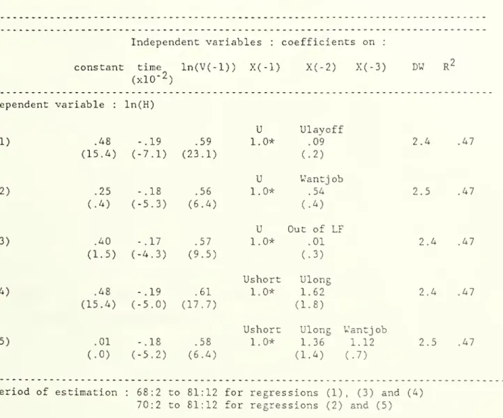
The apprepate matching function: the relevant pool of workers
Our initial specification is based on the joint assumptions of an homogenous pool of
workers, and that the relevant pool of workers is proportional to total unemployment
minus layoff unemployment. Table 3 explores alternative definitions of the pool,
allowing for different types of workers to be perfect substitutes up to a scalar level.
That is, the regressions assume a relation of the form:
ln(Hj.) - a + b time + c ln(V^.-]^) + (l-c)ln(X-L^.-]_ +dX2^-.]L) "''
^t
where X-^ and Xo denote two components of the pool, and are assumed to be perfect
substitutes up to a scale parameter d. All regressions assume constant returns to
scale.
None of the regressions yields precise estimates of the composition of the pool.
The point estimates are nevertheless interesting.
The first regression examines the role of those unemployed classified as job losers
on layoff, a group which was given a weight of zero in the basic specification. The
point estimate of d is 9%, suggesting that some of those workers are also looking for
jobs . The second regression examines the role of those classified as out of the labor
Katz and Meyer (1987) find that workers not expecting to be recalled spend roughly
twice as much time searching as those expecting to be recalled. The study however
Table 3. The aggregate matching function
Alternative definitions of the pool
Independent variables : coefficients on :
constant time ln(V(-l)) X(-l) X(-2) X(-3) DW R^ (xlO-2) Dependent variable : ln(H) U Ulayoff (1) .48 -.19 .59 1.0* .09 2.4 .47 (15.4) (-7.1) (23.1) (.2) U Wantjob (2) .25 -.18 .55 1.0* .54 2.5 .47 (.4) (-5.3) (6.4) (.4) U Out of LF (3) .40 -.17 .57 1.0* .01 2.4 .47 (1.5) (-4.3) (9.5) (.3) Ushort Ulong (4) .48 -.19 .61 1.0* 1.62 2.4 .47 (15.4) (-5.0) (17.7) (1.8)
Ushorc Ulong Wantjob
(5) .01 -.18 .58 1.0* 1.36 1.12 2.5 .47
(.0) (-5.2) (6.4) (1.4) (.7)
Period of estimation : 68:2 to 81:12 for regressions (1), (3) and (4)
70:2 to 81:12 for regressions (2) and (5)
The specification is of the form.:
ln(H) = a + b time + c ln(V(-l) + (l-c)ln (d]_X2^(-l) -t- d2X2(-l) + d3X3(-l)-H£
It is estimated by non linear least squares.
16
force but who indicate that, while they are not looking, they "want a job now"; this
group is slightly larger on average than the pool of those classified as unemployed.
The series is available only quarterly and needs to be interpolated; this probably
reduces its usefulness in regressions. The estimated scale coefficient on this group
is 5A%, confirming the evidence from the flow data that many in this group are
indistinguishable from the unemployed. The next regression, which uses the series for
all those out of the labor force yields essentially a zero scale parameter.
Regressions 4 and 5 consider the separate roles of the short term (less than 27
weeks) and long term unemployed. The first set of results is surprising, finding a
scale parameter on the long term unemployed in excess of unity. One tentative
explanation is that long term unemployment is a better proxy for the pool of workers
out of the labor force, and thus has a coefficient which is biased upwards. Regression
5 attempts to control for that by allowing for short term unemployment, long term
unemployment and workers out of the labor force who want a job. Long term unemployment
still has a scale coefficient which exceeds one. Thus the evidence, while
statistically weak, does not suggest that short term and long term unemployed enter the
matching function differently .
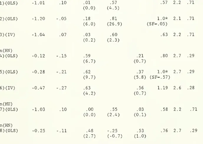
Hires from unemploNinent and out of the labor force
Katz (1986) finds no evidence of a declining job finding hazard once the recall
hazard is taken into account. The evidence appears quite different in the UK, which
has had a very different history of unem.ployment. See for example Jackman and Layard
17
The assumption made in table 3 that the various groups are the same up to a scalar
is not very satisfactory. As hires from unemployment and from out of the labor force
are available separately, we can relax the assumption further and look at the
respective role of the two groups in the matching process.
Figure 2 shows the behavior of the pool of unemployed, U, and the pool of workers
out of the labor force, N. U is defined as above. N is taken to be those workers "out
of the labor force but wanting a job". The series is available from 1970 on. (For
ease of interpretation and comparison to the flows, U and N are divided by 10 in the
figure). The figure also shows the flow of hires from unemployment, HU, and from out
of the labor force, HN. These flows are the CPS flows adjusted by Abowd and Zellner.
HU is further modified to eliminate recalls, as explained earlier. The recall series
is available until 1981, so that the figure and the regressions below are for the
period 1970-1981. As we mentioned earlier, the flows have a large white noise
component, due mostly to sampling error. The series plotted in figure 2 are centered
12-month moving averages of the original series. Figure 3 shows the exit rates from
each of the two pools, using the filtered hire series, HU/U and HN/N.
A number of features clearly emerge from the two figures. The first is that the two
pools, N and U have similar cyclical behavior, the movements in N being of smaller
amplitude. The second is that the flows HU and HN have sharply different cyclical
behavior. The flow of hires from unemployment is highly countercyclical, the flow of
hires from out of the labor force procyclical. The third is that the exit rates are
both procyclical. VThile HU increases when unemployment increases, the elasticity of HU
to U is less than one, so that the exit rate still decreases with the level of
unemployment. But the decline in the exit rate is much more dramatic for those out of
o
3: --J -J en -0 en CD U3 03O
LO (_ Z2 LO (_ zr LO L_ rs: LO L_n
LO L_ Z2 LO C_ ZI LO L_ 12 LO [_ LO L_ IS LO CO hJ _n en CO ' 1o
ro -E en a^
/\
/'l
•^
X
) / .^
V
/
<\
\ < ( /^\
; /l<
< 1 I ^-> 1 / ( >\l
{\
\
^
( ~> > ) \/
/I 1\
-\)
*^,^ ^[ \J
\> <V-A
f
-i
/ \ I/
/\
_ .1 \^
W
1
\s
\
( />
c^^^ \ ~? ~"j\ \ / -1 > >o
m
m
X
X
I I ~-J --0 j: CD CO LD COo
(_ L_ LO (_ IS LQ C_ :z LO t_ IT CO t_ z^ LO (_ ::s LO L_H
LO C_ LO (_ :s LO COTable 4. The aggregate matching function
Looking at the two pools separately
Independent variables : coefficients on
time (xlO-2)
constant time ln(V(-l)) ln(U(-l)) ln(N(-l) RTS DW R^
Dependent variable : In(HU) (1)(0LS) -1.01 .10 .01 .57 .57 2.2 .71 (0.0) (4.5) (2)(0LS) -1.20 -.05 .18 .81 1.0* 2.1 .71 (6.0) (26.9) (SF=.05) (3)(IV) -1.04 .07 .03 .60 .63 2.2 .71 In(HN) (4)(0LS) -0.12 -.15 .59 .21 .80 2.7 .29 (0.7) (5)(0LS) -0.28 -.21 .62 .37 1.0* 2.7 .29 (5.8) (SF=.57) (6)(IV) -0.47 -.27 .63 .56 1.19 2.6 .28 (0.7) In(HU) (7)(0LS) -1.03 .10 .00 .55 .03 .58 2.2 .71 (0.0) (2.4) (0.1) In(HN) (8)(0LS) -0.25 -.11 .48 -.25 .53 .76 2.7 .29 (2.7) (-0.7) (1.0) Period of estimation : 70:2 to 81:12 t statistics in parentheses
Instruments for (3) , (6) : In(IP) , lagged one to three times
;
IP : industrial production
RTS denotes the estimated degree of returns to scale
A star indicates that constant returns was imposed in estimation.
SF is the significance level of the test that returns are constant.
.03 .60 (0.2) (2.3) .59 (5.7) .62 (9.7) .63 (4.2)
labor force is on average higher than that from unemployment : this is implausible and
suggests that the pool of those out of the labor force but wanting a job actually
underestimates the size of the relevant pool of workers out of the labor force.
Table 4 in turn gives a number of simple regressions. Matching functions do not
have a simple functional form when there are two types of workers, with possibly
different search intensity by type, and possibly ranking of the two types by firms when
there are multiple applications. Thus, the log linear specifications of table 4 which
give hires from each pool as a function of the two pools and of vacancies (all in
logarithms) should be taken only as data descriptions, or as log-linear approximations
to yet underived matching functions. Two main features emerge from the table, the lack
of significance of vacancies in explaining hires from unemployment, and the strong
significance of vacancies in explaining hires from out of the labor force.
How may one interpret those facts? Ve can think of workers in the two pools as
differing in three ways. They may differ in how their search intensity varies with
market conditions. They may also differ in their rejection rate : firms may choose,
other things equal, an unemployed worker over one who has been out of the labor force.
Finally, the composition of the pools may change, making workers more or less
acceptable to firms. The fact that the exit rate for those out of the labor force
decreases more sharply than for those unemployed as markets conditions deteriorate may
come from any of those sources. It may come from a decrease in the search intensity of
those out of the labor force relative to the unemployed. It may come from a
deterioration of the quality of the pool of those out of the labor force relative to
19
labor force relative to the unemployed. If firms choose the unemployed over others, a
larger number of unemployed workers will make it relatively harder for those out of the
labor force to find and be accepted for jobs. Ue speculate that all those effects are
at work. The fact that the flow from unemployment actually increases when the total
q
flow into employment decreases cannot be generated by the pure ranking effect . The
(weak) statistical evidence presented in the last two regressions of table 4 that,
given vacancies, the pool of unemployed has a negative effect on hires from out of the
labor force, while the reverse is not true is suggestive of ranking effects.
Confirming those speculations requires the derivation of an appropriate matching
function, something we are currently working on.
We now embed the aggregate matching function in a model of the labor market, which
we simulate.
® The model we have in mind is a model in which firms post vacancies and receive a
random number of applications, which can be equal to zero or one or more. What we call
pure ranking is the case where firms, if they have the choice between unemployed
workers and workers from out of the labor force, always choose the unemployed worker.
20
2. A Minimalist Model of Vacancies and Unemployment
To concentrate on the basic implications of large gross flows and an aggregate
matching function, we leave out most of the texture of actual labor markets . We think
of the economy as being composed of identical workers and jobs. Workers can be in one
of three states: let E be the number of employed workers, U the number of unemployed,
and N the number of workers not in the labor force. Drawing a sharper distinction than
exists, we assume that the unemployed look for work, those out of the labor force do
not. We take the labor force, L, as given. The first relevant equation is therefore:
(2) L = E + U
Jobs can also be in one of three states: they can be either filled, unfilled with a
vacancy posted ("vacancies" for short), or unfilled with no vacancy posted ("idle
capacity"). Each job requires one worker. As with workers, we draw a sharper
distinction between unfilled jobs with or without a vacancy posted than is true: only
those jobs for which a vacancy is posted are looking for workers. Let K be the total
number of jobs; F, the number of filled jobs; V, the num.ber of vacancies; and I, the
number of unfilled jobs with no vacancy posted -idle capacity-. Thus,
9
Ours is not the first model of vacancies and unemployment. We build on the early
work of Hansen (1970) and Holt and David (1966). Our work also parallels work by
Pissarides (1985) and (1987). We differ from his approach in treating the number of
potentially productive jobs as given at any point of time; this has important
21
(3) K - F + V + I
Obviously F and E are identically equal. We take K as given and constant. Note that
by taking K and L to be constant, we treat the two sides of the market in asymmetric
fashion: our focus here is on shocks to the supply of jobs, not on shocks which affect
whether workers decide to enter or leave the labor force.
We think of each of the K jobs in the economy as capable of producing a gross (of
wages) revenue of either 1 or 0. Productivity for each job follows a Markov process in
continuous time. A productive job becomes unproductive with flow probability ttq . An
unproductive job becomes productive with flow probability tti . Thus, the times to a
change in productivity are Poisson processes. At any point in time, some jobs become
productive, some jobs become unproductive. Whether newly productive jobs are jobs
which were previously unproductive, or simply new jobs, is purely a matter of
interpretation in the absence of recalls in the model. This is the mechanism we use to
generate the large gross flows of job creation and job destruction that exist in the
economy. By making this process mechanistic (not dependent on underlying decisions) we
have a simpler (albeit less accurate) setting for focusing on the complexity of
aggregate dynamics
.
The equations of motion
We combine these assumptions with the aggregate matching function described above.
To complete the specification, we make the further assumption that job terminations are
That is, in any short interval of time At there is a probability TTQAt of the job
22
not the only source of separations, but also that workers quit jobs at an exogenous,
constant rate, q. We introduce quits partly for the sake of -some- realism, but also
because there is a basic distinction between quits and job terminations in the model.
A quit is associated with the posting of a new vacancy, a job termination is not. Here
again, the distinction is sharper in the model than in actual labor markets, where
quits are often used by firms to reduce their labor force, and are not always replaced.
The assumptions that the quit rate is constant and that all quits are to unemployment,
are both counterf actual, but not central to the issues at hand.
It follows from our assumptions that the behavior of the labor market is given by a
system of two differential equations, which are:
(4) dE/dt = Qra(U,V) - qE - ttqE
(5) dV/dt - -Qm(U,V) + qE + n-^1 - ttqV
We consider these equations in turn, starting with the behavior of employment. When a
job becomes unproductive, there is no reason for the worker to remain on the job.
Thus, the flow from employment to unemployment from this source is equal to ttqE. In
addition, the flow of quits is equal to qE. The flow from unemplojTnent to employment
is equal to new hires.
For a job to produce 1, it must not only be productive but also be matched with a
worker. To do so, a vacancy must be posted and a worker must be recruited. There are
thus two sources of new vacancies. The first, a flow from I to V, comes from the fact
that jobs which were previously unproductive have become productive; this first flow is
equal to tt-j^I. The second, a flow from F to V, comes from the need to replace workers
who quit; it is equal to qE. Vacancies decrease for two reasons: some are filled by
new hires, a flow from V to F; some of the jobs for which vacancies were posted become
unproductive, a flow from V to I. We assume that vacancies become unproductive at the
23
Using the identities above, these equations can be rewritten as a system in
unemployment and vacancies, given K and L:
(6) dU/dt - -Qm(U,V) + (q+TTQ)(L-U)
(7) dV/dt - -Qm(U,V) + (q-Tr^j^)(L-U) + n-^K - (nQ+n-^)V
This account of the labor reallocation process has not mentioned wages. Wages are
likely to affect K and L as well as ttq and t^-^. But we take K, L, ttq and n-^ as given in
this model. Wages could also affect whether or not a meeting between a worker and a
firm actually leads to a hiring, thus affecting m or q. We assume that wages do not
affect matching. That is, we consider a situation where first the worker and the firm
examine whether there is a mutually advantageous opportunity to begin an employment
relationship. If there is, they then negotiate a wage to divide the surplus from the
match with no constraint (e.g. fairness, union contracts, or posted wages) on allowable
bargains. In a richer model with heterogeneous workers, jobs and matches, the nature
of bargaining power between the two sides would affect allocation by affecting
expectations about future opportunities. We ignore such complications, explicitly
assuming homogeneous workers and firms, absorbing the implications of heterogeneity
into the parameters of the model. In this way, we can focus on unemployment and
vacancies, ignoring wage and price dynamics. Then we can examine wage dynamics with
labor market quantities given.
Steady state and dynamics
Setting dU/dt and dV/dt to zero, we have the steady state values of V and U
satisfying:
(8) Q m(U,V) = (q + ttq) (L-U)
V
D
u
24
Figure 4 shows these stationary curves and directions of motion. The relevant
region of the plane has U,V,E and I all non negative. The locus dU/dt - is downward
sloping. It does not hit the V axis given that m is equal to zero if V is equal to
zero. The locus dV/dt=0 need not be monotonic. Nevertheless there is a unique
equilibrium, which is a stable node.
To think of the dynamics of U and V, we have to specify the sources of shocks to the
economy. It is natural to think of changes in ttq and n-^ as the important source of
fluctuations in the system. But looking at changes in one n keeping the other constant
does not appear to be a particularly relevant experiment. We find it more attractive
to think in terms of shocks to aggregate activity and to the degree of reallocation.
For this purpose, we define two other parameters, c and s, in terms of ttq and tti. For
given ttq and ttt , the proportion of potential jobs which are productive in steady state
is given by n-^/(nQ + ttt ) ; we may think of this proportion, which we shall call c (for
cycle) as measuring the degree of aggregate activity (or more precisely potential
aggregate activity, as the proportion of jobs productive and filled will always be less
than c) . In steady state, the instantaneous flow of jobs changing from productive to
unproductive (which equals the reverse flow) , is equal to 7Tq7t-^/(ttq + 7r-|^) times K; we
can think of this ratio, which we shall denote s (for shift), as an index of the
intensity of reallocation in the economy.
Since ttq-s/c and 7r-j^=s/(l-c) , we can rewrite the dynamic system in terms of s and c:
(10) dU/dt = -Q ni(U,V) + (q+(s/c)) (L-U)
(11) dV/dt - -a m(U,V) + q(L-U) - (s/(l-c)
) ) (K-V-L+U) -(s/c)V
These equations provide a dynamic characterization of the Beveridge relation- the
• •
-
A-1
> ino
d
1o
d
\
. too
\
\
d
^^^^
->^^
•O
\;
^^^^:>^
d
^^^^^^=^^
o
d
o
o
d
0.00 0.02 0.04 0.05 o.os 0.10 UT)\^Urt
5"
25
or reallocation shocks. In our BPEA paper, we analyze those dynamics. We just
summarize them here. Changes in aggregate activity, c, lead to opposite movements in
unemployment and vacancies, with dynamics that are generally counterclocVcwise around
the steady state locus. Figure 5 plots the downward sloping locus giving the steady
state values of U and V corresponding to alternative values of c. It also plots the
dynamics of adjustment of U and V to a sine wave in c. Either the steady state locus
or the loops are what most people have in mind when referring to "the" Beveridge curve.
In contrast, changes in the intensity of reallocation, s, or in the effectiveness of
matching, q, move unemployment and vacancies in the same direction, actually along a 45
degree line if the economy starts from a steady state position. This contrast in
directions of motion in response to different shocks is key for the empirical work
reported below. •
The model clearly captures the idea that high unemplo^inent can be due either to
aggregate activity factors, or to structural changes requiring the reallocation of
labor, and the idea that looking at both unemployment and vacancies can shed light on
the sources of unemployment movements. While there are a number of ways in which this
minimalist model can be enriched -and we discuss a number of them in our BPEA paper- it
is fun at this point to return to the estimated matching function and use it to
simulate the economy.
For the simulation showTi in figure 5, we take the matching function to be Cobb
Douglas, with constant returns and coefficient .4 on unemployment. We choose the scale
parameter. A, to be 1.1 (the estimated scale parameter has a trend and goes from 1.30
at the beginning to .95 at the end of the sample). For the rate of quits (remembering
that only quits that are replaced are relevant) we choose .01, which is the minimum
cwiit^t. It. i9e« 9.02.31 AK
O
d
O
O
o
1 193
cycles
)7 55 73 91 109 T27 14-5 153 181time
inmonths
r)'qurc
6
26
approximate sample averages for unemployment, vacancies and mean hires. This leads to
choices of 1.05 for (K/L) , the ratio of potential jobs to workers, .023 for s, the
reallocation parameter, and .925 for the central value of c, the potential activity
level. These values imply an arrival rate of good profitability shocks, ttt , of .307
and an arrival rate of bad profitability shocks, ttq, of .025. The values of q and ttq
imply in turn an average duration of a match of 2.5 years. For the steady state locus,
we let c vary between .88 and .97. To trace out a cycle, we let c be a sine wave
between .90 and .95, with a period of five years. In this simulation, shown in figure
5, at a vacancy rate of 2% for example, unemployment is roughly 1% higher when the
economy is expanding than when it is contracting. With a decrease in the efficiency of
matching, both the steady state locus and the counterclockwise loops would move
diagonally to the northeast. A horizontal shift to the right in both curve and loop
would come from the combination of a decrease in the efficiency of matching and a lower
level for the cycle of aggregate activity.
In figure 6, we show time paths of new hires, m, unemployment and vacancies from a
simulation of the model with a .0018 downward trend in the efficiency of matching.
This figure can be compared with figure 1 which gives the observed time series. To
reproduce the greater rise in unemployment in figure 1 would require a drop in the
average level of aggregate activity, c, in addition to the decline in the matching
27
3. Wage Determination
In the theory underlying the analysis above, wage setting does not prevent a match
from happening if it is mutually profitable. A natural and appealing formalization
with this property is that the surplus from matching a worker and a firm is shared in
some proportion, an assumption of Nash bargaining. We adopt this assumption and
explore its implications.
For notational convenience, we set the flow of benefits of unemployed workers and
vacancies equal to zero. The total flow of benefits from employment is the excess of
net output over the sum of these two flows ; we denote it by y. We consider risk
neutral workers and firms who all face the same interest rate and have the same
expectations about the future. The gain to a worker from becoming employed is the
difference between the expected present discounted value of wages when one is currently
employed and the expected present discounted value of wages when one is currently
unemployed. We denote this difference by D:
(12) D - W^ - W^
where W.: is the expected present discounted value of income in different current
states. The joint gain from beginning the emploNTT.ent relationship is W^ - W^^ + VJ^
-Thus, this analysis can be converted into the more general analysis by adjusting
the wage for the benefit flow when unemployed and adjusting net output for both the .
profit flow (presumably negative) from, a vacancy and the benefit flow from being
'28
W^, where Wr- and W^ are the present discounted values of profit from the ownership of a
job when the job is currently filled and vacant respectively. The problem of
bargaining is to divide this surplus between the two parties. We assume that the
proportional division of surplus does not vary. Thus, we can write
(13) D = Wg - W^ - z(Wf - W^) r- . . .
With both parties risk neutral and using the same discount rate, there are many wage
patterns which will satisfy (13) , provided they have the same expected present
discounted value. We first consider the situation where wages are continuously
renegotiated to continuously satisfy (13) . Thus all employed workers are earning the
same wage
.
•'
To derive the present discounted value equations, we use the standard dynamic
programming or arbitrage equation approach. The discount rate times the present
discounted value is equal to the flow of benefits plus the capital gains from changes
in position and from changes in the parameters of the economy. Thus
(14) rWg = w + (^o+q)(Wu-^'e) + dW^/dt
rW^ = (Qm/U)(Wg-W^) + dW^/dt
That is, when employed one receives the wage w, the employment relationship ends with
flow probability (ttq + q) , the sum of the rates of bad productivity shocks and
exogenous quits, and the va].ue of being employed changes as the unemployment and
12
vacancy rates change . When unemployed, one is receiving no benefit flow (by
normalization) and one has the flow probability am/U of finding a job. Similarly, we
have
12
29
(15) rW£ - y - w + nQ (W^-W^) + q (W^-W^) + dW^/dt
rW^ - (am/V)(Wf-W^) + ttqCW^-W^) + dW^/dt
rW^ - y' + TT-^ (W^-W^) + dW^/dt
where y' is the saving in costs from idling capacity rather than searching for a worker
and keeping capacity ready to produce.
Subtracting the equations in (lA) and (15) and using the definition of D in (13) as
well as the time derivative of (13) we have
(16) (r+7ro+q+(Qm/U)) D - w + dD/dt
(r+5T-o+q+(Qm/V)) D - z(y-w) + dD/dt
From (16), we obtain an equation relating the wage to the gain from becoming employed
and a differential equation for that gain. These can be rewritten as:
(17) (1+z) w - zy + [(am/V)-(am/V)] D
(1+z) dD/dt - [(l+z)(r+7ro+q)+(Qm/V)+z(am/U)]D - zy
In steady state, i.e. when D is constant, the wage reduces to the simpler expression:
(18) w/y -= (r+7ro+q+am/U)z/((r+7rQ+q) (l+z)+z(am/U)+Qra/V))
Finally, if we assume Qra/ll and am/V to be large compared to r, :t-q and q, w is
approximately equal to:
(18') w s y(zV/(zV+U))
VJhile equation (18') only holds as an approximation and in steady state, it is
likely to be a good approximation to the wage even out of steady state. This is
because (Qm/\') and thus the discount rate in the second equation in (17) is large, so
that the future does not matter very much, and because r, ttq and q are small compared
to the values of am/U and am/v"^^
.
13
With monthly data, am/U is equal to approximately 30%, am/V equal to approximately
&*USSA£lf :«. i»e 1V4i,07 AW
th
=
.5
O
O
^
—
^
O
/
^
\
o
-.r-y—
--^
\
o
-/-^
\-:^;^~\~-—
^
O
'/
^^^nT'^^
/
O
CM\^
/O
o
—
-o
o
o
6
1 7 1 o iS 25 3i 37 45 55 61time
inmonths
T)'^i/yc
7
30
Equation (18') shows how the wage moves with the vacancy/unemployment ratio, which
reflects the arrival rates of alternative opportunities, and with the bargaining
parameter z. Thus changes in aggregate activity, by moving unemployment and vacancies
in opposite directions, will have a strong impact on the wage. But changes in
reallocation, by moving unemployment and vacancies in the same direction, will have a
much smaller effect on the wage.
Equation (17) together with the equations of motion for U and V derived in the
previous section give a characterization of the joint dynamics of U, V and w given c, s
and z. A natural step is to return to the simulation of the last section, which
examines the effects of cyclical movements in c. This is done in figure 7, using
values of 1 for y, 1 for z and .A% per month for the real interest rate.
A striking feature of the figure is the large procyclical movement in w over the c
cycle, an unpleasant implication in view of the actual behavior of the wage. However,
as we mentioned earlier, there is no reason why the wage should always be equal to the
instantaneous wage derived in (17). New matches may well agree to pay a constant real
wage over some (possibly stochastic) time period, with the wage chosen in new matches
equal to the annuity value of the wage in (17) . For example, there might be a
constant real wage for the life of the match. This will substantially decrease the
amplitude both of the wage on new contracts, plotted as wt in figure 7, and of the
current average wage, the average of the wages in force in existing matches, w^ in
Although in this case, we have to add the assumption that workers do not quit to
improve their lot, a possibility which arises when wages are not equal and worVcers are
31
figure 7. The addition of a constant positive value of time when unemployed would
reduce the size of the proportional fluctuations in the wage, since wages would equal
this constant plus the calculated fraction of the excess of output over this constant.
Similarly and moving towards the introduction of nominal rigidities, it is easy to
consider contracts that are fixed in nominal terms for, say, a year and then calculate
the average nominal wage in force at any point.
Even with those extensions, this theory of wage determination does not capture
important aspects of the labor market. A more ambitious task would be to consider wage
setting mechanisms which may sometimes prevent mutually beneficial matching from taking
place. We have in mind here preset wages or union-negotiated wages. Indeed one of the
challenges of this approach is to combine partially centralized wage setting -which we
observe along with wage drift- and a description of the market which allows for the
32
4. Looking at unemployinent, vacancies and wages.
The last two sections have developed a view of fluctuations in unemployment,
vacancies and wages as coming from movements in aggregate activity, in the intensity or
effectiveness of reallocation, in the bargaining power of workers and firms, and in
productivity y. The model is simple, leaving many important aspects of the labor
market out; even so, it suggests an appealing empirical strategy if our goal is to
understand the origins of movements in unemployment.
Define the Beveridge curve and the Phillips curve as the loci traced by unemployment
and vacancies, and by unemployment and wages -leaving again aside the delicate issues
of nominal versus real wages- in response to changes in c. Thus, by definition,
movements in c lead to movements along the Beveridge curve and along the Phillips
curve. In contrast, changes in reallocation intensity or effectiveness lead to shifts
in both the Beveridge curve and the Phillips cur\'e. Changes in bargaining power lead
to shifts in the Phillips curve, but not in the Beveridge curve. One can think of more
complex patterns : a long period of low aggregate activity which leads to a decrease in
the effectiveness of matching will lead to movements along the curves as well as shifts
in the two curves. Thus, by looking at movements on and shifts in the curves, we can
learn something about the sources of fluctuations. This was the avenue explored by
Solow in his Wicksell lectures (1964) . A similar approach has been used more recently
by Layard and Nickell in their analysis of unemployment in the UK (1986).
We have not yet put together a full story along these lines for the US. One obvious
problem is the need to go from the wage equation in (17) to an equation which
33
nature of productivity. But we have started. First, we have looked at the Beveridge
relation to learn about the relative importance and the dynamic effects of the
different shocks. With its recursive structure, our model suggests that we can indeed
look at the Beveridge relation by itself. And we have peeked at the wage equation.
The Beveridge curve
The relation between monthly unemplo^^Tnent and vacancy rates in the US over the
period A8:l to 88:12, using the same measure of vacancies as in Section 1, is plotted
in figure 8. The relation has two clear features. The first is the large thin loops
around a downward sloping locus. The other is the shift to the right over the post war
period. This shift has been well documented (Abraham and Medoff (1982) for example).
Interestingly, it has substantially reversed over the last four years: from 84:12 to
88:12, the vacancy rate has remained roughly constant while the unemployment rate has
decreased by 2%.
Our approach suggests a simple interpretation, one which has been given by Abraham
and Katz (1986): the large loops suggest that aggregate activity shocks dominate short
and medium run movements in unemployment. The shifts to the right and then to the left
suggest a role for changes in reallocation intensity or effectiveness, but at lower
frequencies. What we now present uses more formal econometric techniques but reaches
the same basic conclusions. Our presentation is informal and the reader is referred to
our BPEA paper for details.
We consider the joint behavior of U, V and L. While we assumed in our formalization
that the labor force was constant, we now need to relax this assumption: we saw earlier
34
endogeneity of the labor force with respect to employment is a well documented part of
Okun's law. We assume that movements in U, V and L come from their dynamic responses
to three types of shocks, aggregate activity shocks, c, changes in reallocation
intensity or effectiveness, s (or q, as they have the same dynamic effects), and
exogenous changes in the labor force, f. Those shocks are in turn assumed to follow
stochastic processes with white noise innovations e„, €g and e^ respectively. When we
look at the joint behavior of U, V and L, as characterized by a VAR, we can therefore
think of the innovations in U, V and L as being linear combinations of the three e's.
To achieve identification of the e's, we make a number of identifying restrictions.
The two essential ones are the following. ' •
First, we assume the e's to be mutually uncorrelated. While this is unlikely to be
true, we think of them as coming from largely different sources so that the assumption
is an acceptable first approximation. Second, we assume that c innovations affect
unemployment and vacancies in opposite directions for at least nine months, and that s
innovations affect unemployment and vacancies in the same directions for at least nine
months. This in effect defines the two types of innovations. These restrictions are
sufficient to pin down fairly precisely the e's. Once this is done, it is easy to
decompose the movements in the unemployment and vacancy rates into those parts which
are due to each of the three shocks. Figures 9a to 9d decompose the historical
movements in the unemployment and vacancy rates into the components due to each shock
and to the deterministic component -the movement in unemployment and vacancy rates
which would have occurred, had all realizations of shocks been identically equal to
zero during the period. Those figures confirm and extend our earlier visual
impression.
In the short and medium run, aggregate activity shocks have, by far, the largest
^
^Ur<. ^s VJ q <7» '-"^ r 00 00 CO 00 1 1 CM OJm
in in>
0) O>
<^l^i
0)^
dl !m31 ° E cr ZDM
Q.3
O
bJIp
E co
•O
.yo
ZDO
o
•^3
Q
Z
^Z
C/^ oO
bJ s bJ r or s'2 03 SI' o s 9}Dy Xduddd/\ ,_^ ^^ ^ -<3 CO CO 1 q C7> 1 CM lO cr >r>>
cy O <•—
Q:: •• c Z) /^ o p -/
\ "> >>Q
=' \ _o Q. LJ EU
CJ3
A cQ-
--^ \Q
y
7
>/
LJ *n r q I r OT s: o'c si o 3)0y ADUODDA I ST OT S'Z ^ OT P,Oy ADUCDOA35
counterclockwise loops. Reallocation and labor force shocks have small effects, and
the movements implied by reallocation shocks are initially much flatter than the
movements along a A5 degree line predicted by the theory. There are large flows of job
creation and destruction in the US, but changes in the intensity of the reallocation
process do not appear to be an important determinant of short run unemployment
fluctuations
.
However, part of the longer run shift in the Beveridge relation in the post war
period is attributable to the long run effects of reallocation shocks. The movements
due to changes in aggregate activity, given in figure 9a, are large but, interestingly,
account for none of the drift in the relation over the period. The movements due to
labor force shocks in figure 9b account for small movements of UR and VR and again for
none of the drift. The movements due to changes in reallocation activity or
effectiveness, given in figure 9c, however account for a steady movement of the
unemployment rate upwards, by 2% from the late 60's to 1984, followed by a decrease of
roughly 1% since. Long run effects of reallocation shocks however are not the whole
story. The deterministic component, given in figure 9d, traces an increase in
unemployment of 3% from the early 50's to 1984, followed again by a decrease of 1%
since, without much change in the vacancy rate over the whole period. VThere does the
deterministic component in turn come from? It may come from trends in the underlying
shocks, such as, for example, movements in reallocation intensity steady enough to be
captured by a deterministic rather than by the stochastic component, or from trend
changes in matching, such as for example an increased geographical dispersion of
workers and new jobs. The evidence presented earlier suggests that trend changes in
matching, which we find in our estimation of the matching function for the period 1968