HAL Id: hal-02382546
https://hal.archives-ouvertes.fr/hal-02382546
Submitted on 16 Sep 2020
HAL is a multi-disciplinary open access
archive for the deposit and dissemination of
sci-entific research documents, whether they are
pub-lished or not. The documents may come from
teaching and research institutions in France or
abroad, or from public or private research centers.
L’archive ouverte pluridisciplinaire HAL, est
destinée au dépôt et à la diffusion de documents
scientifiques de niveau recherche, publiés ou non,
émanant des établissements d’enseignement et de
recherche français ou étrangers, des laboratoires
publics ou privés.
Atlantic Subpolar Ocean
Virginie Racapé, Patricia Zunino, Herlé Mercier, Pascale Lherminier, Laurent
Bopp, Fiz Pérez, Marion Gehlen
To cite this version:
Virginie Racapé, Patricia Zunino, Herlé Mercier, Pascale Lherminier, Laurent Bopp, et al.. Transport
and storage of anthropogenic C in the North Atlantic Subpolar Ocean. Biogeosciences, European
Geosciences Union, 2018, 15 (14), pp.4661-4682. �10.5194/bg-15-4661-2018�. �hal-02382546�
https://doi.org/10.5194/bg-15-4661-2018 © Author(s) 2018. This work is distributed under the Creative Commons Attribution 3.0 License.
Transport and storage of anthropogenic C in the North
Atlantic Subpolar Ocean
Virginie Racapé1,2, Patricia Zunino3, Herlé Mercier3, Pascale Lherminier2, Laurent Bopp1,4, Fiz F. Pérèz5, and
Marion Gehlen1
1LSCE/IPSL, Laboratoire des Sciences du Climat et de l’environnement, CEA-CNRS-UVSQ, Orme des Merisiers,
Bât. 712, CEA/Saclay, 91190 Gif-sur-Yvette, CEDEX, France
2IFREMER, Laboratoire d’Océanographie Physique et Spatiale, UMR 6523, CNRS-IFREMER-IRD-UBO, Plouzané, France
3CNRS, Laboratoire d’Océanographie Physique et Spatiale, UMR 6523, CNRS-IFREMER-IRD-UBO, Plouzané, France
4Département de Géosciences, Ecole Normale Supérieure, 24 rue Lhomond, 75005 Paris, France 5Instituto de Investigaciones Marinas, CSIC, Eduardo Cabello 6, 36208 Vigo, Spain
Correspondence: Virginie Racapé (virginie.racape@ifremer.fr) Received: 12 December 2016 – Discussion started: 4 January 2017 Revised: 13 April 2018 – Accepted: 9 June 2018 – Published: 30 July 2018
Abstract. The North Atlantic Ocean is a major sink region for atmospheric CO2 and contributes to the storage of
an-thropogenic carbon (Cant). While there is general agreement that the intensity of the meridional overturning circulation (MOC) modulates uptake, transport and storage of Cant in the North Atlantic Subpolar Ocean, processes controlling their recent variability and evolution over the 21st century remain uncertain. This study investigates the relationship be-tween transport, air–sea flux and storage rate of Cant in the North Atlantic Subpolar Ocean over the past 53 years. Its re-lies on the combined analysis of a multiannual in situ data set and outputs from a global biogeochemical ocean general circulation model (NEMO–PISCES) at 1/2◦spatial resolu-tion forced by an atmospheric reanalysis. Despite an under-estimation of Cant transport and an overunder-estimation of an-thropogenic air–sea CO2flux in the model, the interannual
variability of the regional Cant storage rate and its driving processes were well simulated by the model. Analysis of the multi-decadal simulation revealed that the MOC intensity variability was the major driver of the Cant transport vari-ability at 25 and 36◦N, but not at OVIDE. At the subpolar OVIDE section, the interannual variability of Cant transport was controlled by the accumulation of Cant in the MOC up-per limb. At multi-decadal timescales, long-term changes in the North Atlantic storage rate of Cant were driven by the increase in air–sea fluxes of anthropogenic CO2. North
At-lantic Central Water played a key role for storing Cant in the
upper layer of the subtropical region and for supplying Cant to Intermediate Water and North Atlantic Deep Water. The transfer of Cant from surface to deep waters occurred mainly north of the OVIDE section. Most of the Cant transferred to the deep ocean was stored in the subpolar region, while the remainder was exported to the subtropical gyre within the lower MOC.
1 Introduction
Since the start of the industrial era and the concomitant rise of atmospheric CO2, the ocean sink and inventory of
anthro-pogenic carbon (Cant) have increased substantially (Sabine et al., 2004; Le Quéré et al., 2009, 2014; Khatiwala et al., 2013). Overall, the ocean absorbed 28 ± 5 % of all anthro-pogenic CO2emissions, thus providing a negative feedback
to global warming and climate change (Ciais et al., 2013). Uptake and storage of Cant are nevertheless characterized by a significant and poorly understood variability on interannual to decadal timescales (Le Quéré et al., 2015; Wanninkhof et al., 2013). Any global assessment hides important regional differences, which could hamper detection of changes in the ocean sink in response to global warming and unabated CO2
emissions (Séférian et al., 2014; McKinley et al., 2016). The North Atlantic Ocean is a key region for Cant up-take and storage (Sabine et al., 2004; Mikaloff-Fletcher et
al., 2006; Gruber et al., 2009; Khatiwala et al., 2013). In this region, storage of Cant results from the combination of two processes: (1) the northward transport of warm and Cant-laden tropical waters by the upper limb of the merid-ional overturning circulation (MOC; Álvarez et al., 2004; Mikaloff-Fletcher., 2006; Gruber et al., 2009; Pérez et al., 2013) and (2) deep winter convection in the Labrador and Irminger seas, which efficiently transfers Cant from surface waters to the deep ocean (Körtzinger et al., 1999; Sabine et al., 2004; Pérez et al., 2008). Both processes are character-ized by high temporal variability in response to the leading mode of atmospheric variability in the North Atlantic, the North Atlantic Oscillation (NAO). Hurrell (1995) defined the NAO index as the normalized sea-level pressure difference in winter between the Azores and Iceland. A positive (negative) NAO phase is characterized by a high (low) pressure gradient between these two systems corresponding to strong (weak) westerly winds in the subpolar region. Between the mid-1960s and the mid-1990s, the NAO changed from a negative to a positive phase. The change in wind conditions induced an acceleration of the North Atlantic Current (NAC), as well as increased heat loss and vertical mixing in the subpolar gyre (e.g., Dickson et al., 1996; Curry and McCartney, 2001; Sarafanov, 2009; Delworth and Zeng, 2016). Concomitant enhanced deep convection led to the formation of large vol-umes of Labrador Sea Water (LSW) with a high load of Cant (Lazier et al., 2002; Pickart et al., 2003; Pérez et al., 2008, 2013). Between 1997 and the early 2010s, the NAO index declined, causing a reduction in LSW formation (Yashayaev, 2007; Rhein et al., 2011) and a slowdown of the northward transport of subtropical waters by the NAC (Häkkinen and Rhines, 2004; Bryden et al., 2005; Pérez et al., 2013). As a result, the increase in the subpolar Cant inventory was below values expected solely from rising anthropogenic CO2levels
in the atmosphere (Steinfeldt et al., 2009; Pérez et al., 2013). Based on the analysis of time series of physical and bio-geochemical properties between 1997 and 2006, Pérez et al. (2013) proposed that Cant storage rates in the subpo-lar gyre were primarily controlled by the intensity of the MOC. A weakening of the MOC would lead to a decrease in Cant storage and would give rise to a positive climate– carbon feedback. The importance of the MOC in modulating the North Atlantic Cant inventory was previously suggested by model studies, which projected a decrease in the North At-lantic Cant inventory over the 21st century in response to a MOC slowdown under climate warming (e.g., Maier-Reimer et al., 1996; Crueger et al., 2008; Schwinger et al., 2014). Zunino et al. (2014) extended the time window of analysis of Pérez et al. (2013) to 1997–2010. They proposed a novel proxy for Cant transport defined as the difference of Cant concentration between the upper and the lower limbs of the overturning circulation times the MOC intensity (please re-fer to the Supplement (Sect. S1) for a model-based discus-sion of the proxy and for the MOC intensity definition). The authors concluded that while the interannual variability of
Cant transport across the OVIDE section was controlled by the variability of the MOC intensity, its long-term change depended on the increase in Cant concentration in the up-per limb of the MOC. The latter reflects the uptake of Cant through gas exchange at the atmosphere–ocean boundary and questions the dominant role attributed to ocean dynamics in controlling Cant storage in the subpolar gyre at decadal and longer timescales (Pérez et al., 2013). Were the storage rate of Cant in the subpolar gyre indeed controlled at first order by the load of Cant in the upper limb of the MOC, the increase in the subpolar Cant inventory would follow the increase in atmospheric CO2 over the 21st century despite a projected
weakening of the intensity of MOC (Collins et al., 2013). The objective of this study is to evaluate the variability of transport, air–sea flux and storage rate of Cant in the North Atlantic Subpolar Ocean and its drivers over the past 53 years (1959–2011). It relies on the combination of a multi-annual data set representative of the area gathered from 25◦N to
the Greenland–Iceland–Scotland sills over the period 2003– 2011 and outputs from the global biogeochemical ocean gen-eral circulation model NEMO–PISCES at 1/2◦spatial reso-lution forced by an atmospheric reanalysis (Bourgeois et al., 2016). The paper is organized as follows.
NEMO–PISCES and the in situ data are introduced in Sect. 2 and compared in Sect. 3 to evaluate model perfor-mance. An analysis of mechanisms controlling the interan-nual to decadal variability of the regional Cant fluxes and storage rate is presented in Sect. 4, and results are discussed in Sect. 5.
2 Material and methods
2.1 NEMO–PISCES model
This study is based on a global configuration of the ocean model system NEMO (Nucleus For European Modelling of the Ocean) version 3.2 (Madec, 2008). The quasi-isotropic tripolar grid ORCA (Madec and Imbard, 1996) has a res-olution of 0.5◦ in longitude and 0.5◦×cos(ϕ) in latitude (ORCA05) and 46 vertical levels whereof 10 levels lie in the upper 100 m. It is coupled online to the Louvain-la-Neuve sea ice model version 2 (LIM2) and the biogeochemical model PISCES-v1 (Pelagic Interaction Scheme for Carbon and Ecosystem Studies; Aumont and Bopp, 2006). Parame-ter values and numerical options for the physical model fol-low Barnier et al. (2006) and Timmermann et al. (2005). Two atmospheric reanalysis products, DFS4.2 and DFS4.4, were used for this study. DFS4.2 is based on ERA-40 (Brodeau et al., 2010) and covers the period 1958–2007, while DFS4.4 is based on ERA-Interim (Dee et al., 2011) and covers the years 2002–2012. The simulation was spun up over a full DFS4.2 forcing cycle (50 years) starting from rest and hold-ing atmospheric CO2 constant to levels of the year 1870
Figure 1. Column inventory (molC m−2)of anthropogenic carbon for the year 2010: (a) model output and (b) Khatiwala et al. (2009).
Figure 2. Locations of the 24.5◦N and OVIDE sections in ORCA05–PISCES (black thick line) and observations (red points).
Barnier et al. (2006). Biogeochemical tracers were either ini-tialized from climatologies (nitrate, phosphate, oxygen, dis-solved silica from the 2001 World Ocean Atlas, Conkright et al., 2002, and preindustrial dissolved inorganic carbon (CT)
and total alkalinity (AT)from GLODAP, Key et al., 2004) or
from a 3000-year-long global NEMO–PISCES simulation at 2◦horizontal resolution (iron and dissolved organic carbon). The remaining biogeochemical tracers were initialized with constant values.
At the end of the spin-up cycle, two 143-year long sim-ulations were started in 1870 and run in parallel. The first one, the historical simulation, was forced with spatially
uniform and temporally increasing atmospheric CO2
con-centrations (Le Quéré et al., 2014). In the second simu-lation, the natural simusimu-lation, the mole fraction of atmo-spheric CO2was kept constant in time at 287 ppm. Both runs
were forced by repeating 1.75 cycles of DFS4.2, interannu-ally varying forcing over 1870 to 1957. Next DFS4.2 was used from 1958 to 2007. Simulations were extended up to 2012 by switching to DFS4.4 in 2002. No significant dif-ferences were found in tracer distributions and Cant related quantities between both atmospheric forcing products dur-ing the years of overlap (2002–2007). Carbonate chemistry
and air–sea CO2fluxes were computed by PISCES
follow-ing the Ocean Carbon Cycle Model Intercomparison Project protocols (http://ocmip5.ipsl.jussieu.fr/OCMIP/, last access: 25 June 2018) and the gas transfer velocity relation provided by Wanninkhof (1992). Climate change trends and natural modes of variability are part of the forcing set used to force both simulations. Hence, any alteration of the natural car-bon cycle in response to climate change (e.g., rising sea sur-face temperature) will be part of the natural simulation. The concentration of Cant, as well as anthropogenic CO2fluxes,
is calculated as the difference between the historical (total C = natural + anthropogenic contribution) and natural simu-lations following Orr et al. (2017).
The model simulates a global ocean inventory of Cant in 2010 of 126 PgC. It is at the lower end of the uncer-tainty range of the estimate by Khatiwala et al. (2013) of 155 ± 31 PgC (Fig. 1). At the global scale, the error of the model is close to 6 % (values excluding arctic region and marginal seas). The underestimation of the simulated Cant inventory compared to Khatiwala et al. (2013) is largely ex-plained by the difference in the starting year of integration (Bronselaer et al., 2017): 1870 for this study as opposed to 1765 in Khatiwala et al. (2013). The coupled model con-figuration is referred to as ORCA05–PISCES hereafter. The reader is referred to Bourgeois et al. (2016) for a detailed description of the model and the simulation strategy.
Table 1. References of cruises used in this study.
OVIDE name Month/year Vessel Reference Expocode
OVIDE 2002 06–07/2002 N/O Thalassa Lherminier et al. (2007) 35TH20020611
OVIDE 2004 06–07/2004 N/O Thalassa Lherminier et al. (2010) 35TH20040604
OVIDE 2006 05–06/2006 R/V Maria S. Merian Gourcuff et al. (2011) 06MM20060523
OVIDE 2008 06–07/2008 N/O Thalassa Mercier et al. (2015) 35TH20080610
OVIDE 2010 06–07/2010 N/O Thalassa Mercier et al. (2015) 35TH20100608
24.5◦N–2011 01–03/2011 Sarmiento de Gamboa Hernández-Guerra et al. (2014) 29AH20110128
2.2 Observational data sets
Observations used to evaluate the transport of Cant in ORCA05–PISCES were collected along the Greenland– Portugal OVIDE section and at 24.5◦N following the tracks
presented in Fig. 2. Simulated air–sea fluxes of CO2 were
compared to the observation-based gridded sea surface prod-uct of air–sea CO2fluxes from Landschützer et al. (2015a).
Programs and/or data sets are briefly summarized below.
2.2.1 OVIDE data set
The OVIDE program aims to document and understand the origin of the interannual to decadal variability in cir-culation and properties of water masses in the North At-lantic Subpolar Ocean in the context of climate change (http://www.umr-lops.fr/Projets/Projets-actifs/OVIDE). Ev-ery 2 years since 2002, one spring–summer cruise was run between Greenland and Portugal (Table 1, Fig. 2). Dynam-ical (ADCP), physDynam-ical (temperature, T , and salinity, S) and biogeochemical (alkalinity, AT, pH, dissolved oxygen, O2,
and nutrients) properties were sampled over the entire water column at about 100 hydrographic stations. An overview of instruments, analytical methods and accuracies of each pa-rameter is presented in Zunino et al. (2014). The concentra-tion of CTwas calculated from pH and ATfollowing the
rec-ommendations and guidelines from Velo et al. (2010). The OVIDE data set is distributed as part of GLODAPv2 (Global Ocean Data Analysis Project; Olsen et al., 2016) (Table 1). 2.2.2 24.5◦N data set
Data were collected along 24.5◦N in 2011 between 27 Jan-uary and 15 March as part of the Malaspina expedition (https: //www.expedicionmalaspina.es, last access: 25 June 2018) (Table 1, Fig. 2). As for the OVIDE program, ADCP, T , S, AT, pH, O2and nutrients were sampled during the cruise and
CT was calculated from ATand pH. For details on methods
and accuracies, the reader is referred to Hernández-Guerra et al. (2014) for dynamical and physical properties and to Guallart et al. (2015) for the carbonate system. This data set is available from CCHDO (Clivar & Carbon Hydrographic Data Office; Table 1).
For both data sets, CT was combined with T , S,
nutri-ents, O2 and AT to derive the Cant concentration
follow-ing the ϕCT method. Preindustrial atmospheric CO2 was
fixed at 278.8 ppm to compute the preindustrial CT (Pérez
et al., 2008; Vàzquez-Rodrìguez et al., 2009). This data-based diagnostic uses water mass properties of the subsur-face layer between 100 and 200 m as reference to evaluate preformed and disequilibrium conditions. An uncertainty of
5.2 µmol kg−1 on Cant values was estimated from random
error propagation in input parameters (Pérez et al., 2010). A comparison between different methods used to separate Cant from natural CT in the Atlantic Ocean (Vàzquez-Rodrìguez
et al., 2009) and along 24.5◦N (Guallart et al., 2015) con-cluded to a good agreement between ϕCTand the other
meth-ods.
2.2.3 Air–sea CO2flux data set
The gridded sea surface pCO2 product of Landschützer et
al. (2015a) is based on version 2 of the SOCAT data set (Bakker et al., 2014) and a two-step neural network method detailed in Landschützer et al. (2015b). It consists of monthly surface ocean pCO2 values from 1982 to 2011 at a spatial
resolution of 1◦×1◦. Total air–sea CO2fluxes were derived
from Eq. (1), where dCO2is defined as the difference of CO2
partial pressures between the atmosphere and surface ocean, Kw is the gas transfer velocity and sol is the CO2solubility.
FCO2sea–air=Kw×sol × dCO2 (1)
Kw was computed following Wanninkhof (1992) as a
func-tion of wind speed and it was rescaled to a global mean gas transfer velocity of 16 cm h−1 using winds from ERA-Interim (Dee et al. 2011) as explained in Landschützer et al. (2014). Following Weiss (1994), sol was computed as a function of sea surface temperature (Reynolds et al., 2002) and sea surface salinity from Hadley Centre EN4 (Good et al. 2013).
2.3 Diagnostic of Cant transport and budget
2.3.1 Transport of Cant across a section
The simulated transport of Cant (TCant)across a section was
simula-tion) or from offline (computed using stored model output) diagnostics. The transport of Cant is the sum of advective, diffusive and eddy terms. These terms were integrated ver-tically from bottom to surface and horizontally from the be-ginning (A) to the end (B) of the section along a continuous line defined by zonal (y) and meridional (x) grid segments (Fig. S2). Positive values stand for northward and/or east-ward transports. The advective term corresponds to the prod-uct of the horizontal velocity orthogonal to the section (V ) times the concentration of Cant ([Cant], Eq. 2).
mTadv Cant= Z B A Z surface bottom V[Cant]dxydz (2)
The diffusive term corresponds to the transport of Cant due to the horizontal diffusion. The subgrid-scale eddy transport was parameterized using Gent and McWilliams (1990). The online approach allowed advective, diffusive and eddy terms to be quantified, while the offline approach only allowed the calculation of the advective term. All terms of TCantwere
di-agnosed from 2003 to 2011, the period for which the online diagnostics were available. Simulated TCantwas compared to
observation-based estimates from 24.5◦N to the Greenland– Iceland–Scotland sills (Sect. 3.1). To study the long-term variability of Cant fluxes and storage rates (Sect. 3.2), the time window of analysis was extended to 1958–2012 and Cant transport was derived offline from yearly averaged model outputs according to Eq. (1).
2.3.2 Budget of Cant in the North Atlantic Ocean
The budget of Cant was computed for several North Atlantic subregions (boxes) defined later on. A budget was defined for each box as the balance between (i) the time rate of change in vertically and horizontally integrated Cant, (ii) the incom-ing and outgoincom-ing transport of Cant across boundaries of each region and (iii) the spatially integrated air–sea flux of an-thropogenic CO2 . The air–sea flux of total CO2 was also
computed over 2003–2011. All terms were estimated either from monthly (2003–2011) or yearly (1958–2012) averages of model outputs depending on the period of analysis. Rela-tionships between Cant fluxes and storage rates were investi-gated for each region.
2.4 Diagnostic of heat transport
Heat transport across a section was computed from horizon-tal velocity orthogonal to the section times the heat term es-timated from temperature and salinity using the international thermodynamic equations of seawater (TEOS 2010). Heat transport is used in Sect. 4.1 to evaluate model performance to reproduce the well-known mechanism controlling its in-terannual variability correctly and to compare to results for Cant transport. 0.092 ± 0.016 0.216 ± 0.019 0.045 ± 0.006 0.303 ± 0.013 0.156 ± 0.008 0.035 ± 0.005 0.034 ± 0.004 0.103 ± 0.006 0.044 ± 0.003 (17.75*1012 m²) (3.51*1012m²) 2 5 ° N O V ID E Sills
Figure 3. Anthropogenic C budget of the North Atlantic Subtropical and Subpolar regions over the period 2003–2011. Average values and their standard deviations were estimated from smoothed time series. Horizontal arrows show total Cant transport in PgC yr−1 (black font). Red numbers indicate Cant storage rate in PgC yr−1. Vertical arrows show the air–sea fluxes of total (blue font) and an-thropogenic (black font) CO2in PgC yr−1. Boundaries and surface
area (m2) of each box are indicated below the panels.
3 Model evaluation over the period 2003–2011
Figure 3 summarizes the budget of Cant in the North At-lantic simulated by the model over the period 2003–2011. In order to enable the comparison of the model-derived budget to previous estimates (e.g., Jeansson et al., 2011; Pérez et al. 2013; Zunino et al., 2014, 2015a, b; Guallart et al., 2015), we defined two boxes separated by the Greenland–Portugal
OVIDE section. The first box extends from 25◦N to the
OVIDE section, and the second box extends from the OVIDE section to the Greenland–Iceland–Scotland sills. Seasonality was removed beforehand using a 12-month running filter.
3.1 Advective transport of Cant
In the model, over one-third of Cant entering in the southern box at 25◦N (0.092 ± 0.016 PgC yr−1)is transported across the OVIDE section before leaving the domain through the Greenland–Iceland–Scotland sills (Fig. 3). The comparison between online and offline estimates of Cant transport across the OVIDE section confirms the dominant contribution of ad-vection (Fig. S3) in line with Tréguier et al. (2006). Simu-lated transport of Cant (Fig. 3) is clearly underestimated: it is 3 times smaller than observations at 25◦N (Zunino et al., 2015b) and at the OVIDE section (Pérez et al., 2013; Zunino et al., 2014, 2015a), whereas it is 1.5 to 2 times smaller than observations at the sills (Jeansson et al., 2011; Pérez et al., 2013). In order to identify the reasons for the underestimation of TCant in the model, simulated volume transport and
con-centration of Cant are compared to in situ estimates (Eq. 2) in the following paragraphs.
3.1.1 Mass transport across the Greenland–Portugal
OVIDE section and 25◦N
Figure 4 shows the accumulated volume transport simulated by ORCA05–PISCES along the Greenland–Portugal sec-tion compared to assessments based on observasec-tions from OVIDE. The simulated intensity of the MOC (see Sect. S1 for details of its estimation) underestimates the observational estimate of 15.5 ± 2.3 Sv (Mercier et al., 2015) for both the month of June (13.4 ± 0.6 Sv) and annual average values (12.7 ± 0.6 Sv vs. 18.1 ± 1.4 Sv in Mercier et al., 2015; Ta-ble 2). The overturning stream function simulated by the model shows an average pattern similar to the observation-based assessment despite a weaker maximum and differences in the transport distributions in the upper limb of the MOC (Fig. 4a). Some of those differences can be explained by ex-amining the horizontal distribution of the transport and asso-ciated variability (Fig. 4b). The NAC, which flows northeast-ward in the upper limb of the MOC (Lherminier et al., 2010), is simulated with a lower variability and weaker intensity than in the observations (15 Sv instead of 25 Sv). The weaker NAC is not compensated by the transport overestimation above σ1=31.5 kg m−3. As a result, the intensity of MOC is
smaller in the model than in the observations. Figure 4b also shows that the model underestimates the cumulative volume transport for σ1>32.40 kg m−3(σ0>27.7 kg m−3), the
lat-ter being close to 0 Sv in the model (Fig. 4a) as opposed to 7 Sv reported by Lherminier et al. (2007) and García-Ibáñez et al. (2015). These high density classes encompass lower North East Atlantic Deep Water (lNEADW), Denmark Strait Overflow Water (DSOW) and Iceland–Scotland Overflow Water (ISOW). Interestingly, the misfit between observation-derived estimates and simulated volume transport is largest in the WBC in the Irminger and in the Iceland basins (Fig. 4b). This suggests that the significant underestimation of volume transport in these high density classes in the model is most likely due to the misrepresentation of Nordic overflows at the latitude of the OVIDE section.
At 25◦N, the upper limb of the MOC, composed of
North Atlantic Central Water (NACW), Antarctic Intermedi-ate WIntermedi-ater (AAIW) and Mediterranean WIntermedi-ater (MW) (Talley et al., 2011; Hernández-Guerra et al., 2014), flows northward, while the lower limb transports North Atlantic Deep Water (NADW) southward and Antarctic Bottom Water northward (AABW; Kuhlbrodt et al., 2007; Talley et al., 2011; Fig. 5b). Over January–March 2011, the MOC upper limb had an in-tensity of 9.0 ± 2.3 Sv in the model (Fig. 5a), while the lower limb showed a net flux of −10.8 ± 2.1 Sv (Fig. 5a). The in-tensity of simulated MOC was weaker (Table 3) than results reported by Hernández-Guerra et al. (2014) for the same pe-riod (Table 3). The magnitude of the simulated annual mean MOC over 2003–2011 (11.1 ± 0.8; Table 3) was also low compared to the estimate from McCarthy et al. (2012) (mean MOC over 2005–2008 of 18.5 ± 1.0 Sv at 26◦N). The large underestimation of the transport of the Nordic overflows is
most likely at the origin of the underestimation of NADW transport and the MOC at 26◦N (Fig. 5a).
3.1.2 Cant distribution in the North Atlantic Ocean
and along the OVIDE section and 25◦N
The simulated spatial distribution of Cant between 25◦N and the Greenland–Iceland–Scotland sills (Fig. 1) is in good agreement with Khatiwala et al. (2013). The compar-ison of Cant concentrations is less satisfying, with an un-derestimation as large as 40 molC m−2 of simulated max-ima. Simulated and observed Cant along the Greenland–
Portugal OVIDE section and 25◦N also display similar
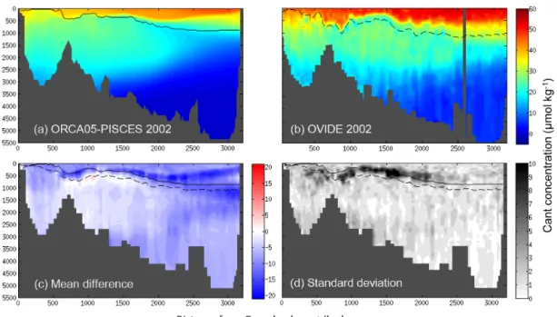
patterns (Figs. 6 and 7). Despite this agreement, simu-lated concentrations along the OVIDE section are lower by 6.3 ± 0.6 µmol kg−1 compared to observation-based es-timates (Table 2). This deficit is more pronounced in the upper MOC (1Cantmodel–data= −5.9 ± 0.7 µmol kg−1)than in the lower MOC (1Cantmodel–data= −3.6 ± 0.6, Table 2). The largest difference between model and data (up to −20 µmol kg−1; Fig. 6c) is detected in subsurface waters at the transition between East North Atlantic Central Water (ENACW) and Mediterranean Water (MW) and between the two limbs of the MOC. Figure 6 also reveals an underestima-tion by the model of Cant levels in lNEADW (below 3500m depth in the western European basin) by 5 to 10 µmol kg−1, which is in line with a transport of Nordic overflow waters across the OVIDE section close to zero. The variability of the model–data differences at OVIDE (Fig. 6d) is the largest at the boundary between the upper and lower limbs of the MOC and between 700 and 2000 km off Greenland. The higher dif-ference in this region is explained by an underestimation of the variability of the NAC intensity by ORCA05–PISCES.
At 25◦N, the model also underestimates the Cant con-centration by more than 10 µmol kg−1 on average, which is mainly due to a large underestimation in the MOC lower limb (Table 3). The largest difference between ORCA05– PISCES and observations, up to −30 µmol kg−1, is neverthe-less found around 500 m depth. It is due to a subsurface ver-tical gradient of Cant that was shallower in the model than in the observations. The simulated averaged Cant content in the MOC upper limb is, however, comparable to the obser-vations (Table 3) because of a compensation due to a thinner upper MOC in the model (Fig. 7a, b). Figure 7 also shows an underestimation of Cant below 3500 m depth by about
10 µmol kg−1within AABW.
To summarize Sect. 3.1, the underestimation of Cant trans-port in ORCA05–PISCES is likely due to the combination of weak volume transports of NAC and Nordic overflows and low Cant concentrations. The latter is partly explained by the preindustrial condition for atmospheric CO2used by the
Figure 4. Volume transport (Sv) across the OVIDE section as simulated by the model for the month of June (continuous line for mean value; shaded band for confidence interval) and compared to the observation-based assessments (dashed line) over the period 2002–2010. In panel (a), the coast-to-coast integrated volume transport was accumulated from the bottom with a 0.01 kg m−3resolution in density referenced to 1000 db (σ1). The sign of the profile was changed to get a positive MOC magnitude. Black horizontal lines indicate the density level
where the MOC magnitude is found in the model (continuous line; σ MOC = 32.02 ± 0.05 kg m−3)and in the observations (dashed line; σMOC = 32.14 kg m−3, Zunino et al., 2014). They also represent the separation between the upper (red) and lower (blue) limbs of the MOC. In panel (b), the volume transport was horizontally accumulated from Greenland to Portugal (km) and vertically integrated over the upper (red) and the lower (blue) limbs of the MOC. Vertical lines represent the limits of the North Atlantic Current (NAC) as reported in Mercier et al., 2015. The position of the western boundary current (WBC) is also indicated.
Table 2. Model–data comparison over the period covered by the OVIDE cruises (2002–2010). Average and standard deviation (SD) for observation-based estimates (column 2) and model output (columns 3 to 4). Model output: (1) June average, with SD being a measure of interannual variability, and (2) yearly average, with SD corresponding to the average interannual variability.
OVIDE ORCA05–PISCES
observations June only Yearly average
MOCσ (Sv) 15.5 ± 2.3 13.4 ± 0.6 12.7 ± 0.6
σMOC (kg m−3) 32.14 32.02 ± 0.05 31.95 ± 0.04
[Cant]section(µmol kg−1) 25.4 ± 1.8 18.4 ± 1.1 18.4 ± 1.1
[Cant]upper(µmol kg−1) 45.2 ± 3.0 38.9 ± 3.0 39.4 ± 3.0
[Cant]lower(µmol kg−1) 19.4 ± 1.6 14.8 ± 1.0 14.9 ± 1.0
3.2 Air–sea fluxes of total and anthropogenic CO2
Simulated air–sea fluxes of total and anthropogenic CO2
(Fig. 3) are higher than those derived from in situ data
by Pérez et al. (2013) their Fig. 3. For total CO2,
the model–data difference is 0.013 PgC yr−1 (northern
box) and 0.103 PgC yr−1 (southern box). For the anthro-pogenic component, it is 0.028 PgC yr−1(northern box) and 0.036 PgC yr−1 (southern box). While the model overesti-mates CO2uptake, the ratio of anthropogenic to natural flux
is comparable to previous estimates (Gruber et al., 2009; Schuster et al., 2013), which implies a similar overestimation
of both components. To understand the origin of the overes-timation of fluxes, simulated air–sea fluxes of total CO2were
averaged over 2003–2011 and compared to observation-based estimates from Landschützer et al. (2015a), taken as representative of the SOCCOM exercise (Rödenbeck et al., 2015). The model overestimates CO2uptake mainly between
the OVIDE section and the Greenland–Iceland–Scotland sills (Fig. 8a, b). The month of occurrence of the seasonal maxi-mum or minimaxi-mum air–sea CO2flux was diagnosed. It is
pre-sented in Fig. 8c, d. A seasonal phase shift between simu-lated fluxes and data-based estimates is observed north of 50◦N, where the model strongly overestimates gas exchange.
Figure 5. Volume transport (Sv) integrated zonally at 24.5◦N. In panel (a), the volume transport was computed in three water mass classes over the period January–March 2011. The three classes encompass (1) North Atlantic Central Water (NACW), Antarctic Intermediate Water (AAIW) and Mediterranean Water (MW) flowing in the upper MOC (red) and (2) North Atlantic Deep Water and (3) Antarctic Bottom Water (AABW) flowing in the lower MOC (blue). Model results (filled bar plot) are compared with the observation-based estimates from Hernández-Guerra et al. (2014) (hatched bar plot). In panel (b), the volume transport was computed in density level (σ1with 0.1 kg m−3
resolution) from model output over the year 2011. Black horizontal lines indicate the density where the MOC magnitude was found in the model over the study period (σ1=32.05 from July to September and σ1=31.95 for other months). They also represent the separation
between the MOC limbs (upper in red, lower in blue).
Table 3. Model–data comparison along 25◦N. Average and standard deviation (SD) for observation-based estimates (column 2) and model output (columns 3 to 5). Model output: (1) January to March 2011 average, with SD being a measure of winter variability, (2) 2011 average, with SD corresponding to the 2011 seasonal variability, and (3) 2003–2011 average, with SD being the interannual variability.
24.5◦N ORCA05–PISCES
observations winter only 2011 average 2003–2011 average
MOCσ (Sv) 20.1 ± 1.4 10.8 ± 2.1 11.6 ± 1.9 11.1 ± 0.8
σMOC (kg m−3) 32.27 31.95 ± 0.00 32.02 ± 0.03 32.00 ± 0.03
[Cant]section(µmol kg−1) 19.73 8.69 ± 0.02 8.73 ± 0.04
[Cant]upper(µmol kg−1) 40.36 39.15 ± 0.01 38.86 ± 0.90
[Cant]lower(µmol kg−1) 12.00 2.89 ± 0.1 2.86 ± 0.08
Fluxes peak in winter in observations, while they reach their maximum in summer in the model. The seasonal change in surface water pCO2 is dominated by biological activity
north of 40◦N and by temperature (or thermodynamics) be-tween 20 and 40◦N (Takahashi et al., 2002). The model
re-produces the main driving process of seasonal variability of air–sea CO2 fluxes in the subtropical region. However, the
dominant effect of temperature extends too far north in the model because the latter failed to reproduce the air–sea gra-dient of winter pCO2. As a result, the seasonal change in
CO2 fluxes is dominated by the thermodynamical effect in
the subpolar gyre, which enhances the ocean sink for atmo-spheric CO2. Despite the seasonal phase shift noted in the
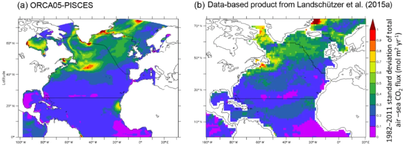
subpolar gyre, the amplitude of the interannual variability of total air–sea CO2fluxes (defined as the standard deviation of
air–sea fluxes computed over 1982–2011 after removing the seasonal cycle; Fig. 9) is well reproduced by the model over the total domain, including north of 40◦N where the
variabil-ity is the largest.
3.2.1 Storage rate of Cant
Over 88 % of the simulated Cant flux entering the North At-lantic between 25◦N and the Greenland–Iceland–Scotland sills (Fig. 3) is stored inside the region, predominantly south of the OVIDE section. The regional convergence of
Figure 6. Water column distribution of anthropogenic C concentrations (µmol kg−1)along the Greenland–Portugal OVIDE section in June 2002: (a) model output and (b) as estimated from the OVIDE data set. The mean and standard deviation of differences between these two assessments (model–observation) over the OVIDE period (June 2002-04-06-08-10) are displayed in panels (c) and (d). Black continuous and dashed lines indicate the limit between the upper and the lower MOC in the model and in the OVIDE data set, respectively.
Figure 7. Water column distribution of anthropogenic C concentrations (µmol kg−1)along 24.5◦N during winter (JFM) 2011: (a) model output and (b) as estimated from the 24.5◦N data set. Differences between the two assessments (model–observation) are displayed in panel (c). Black continuous and dashed lines indicate the limit between the upper and the lower MOC in the model and in the observations.
Figure 8. (a–b) Average total air–sea CO2 fluxes (mol m2yr−1) and months during which (c–d) the maximum or (e–f) the minimum value is reached in the North Atlantic Ocean over the period 2003–2011, as simulated by the ORCA05–PISCES model (left panels) and compared with the data-based estimate from Landschützer et al. (2015a) (right panel). Black lines indicate borders of boxes 25◦N–OVIDE and OVIDE–sills.
Cant transport adds to the strong air–sea flux occurring in the region to explain simulated storage rates for 2003– 2011. The latter are in line with estimates from Pérez et al. (2013) (referenced to 2004: south 0.280 ± 0.011 and north 0.045 ± 0.004 PgC yr−1). These results point towards the compensation in the model between the underestimation of Cant transport and the overestimation of anthropogenic CO2
air–sea fluxes.
Next, the contribution of air–sea uptake and transport of Cant to the variability of the North Atlantic Cant inventory is derived for each box from the analysis of multi-annual time series of air–sea fluxes of anthropogenic CO2, transport
di-vergence of Cant (defined as the difference between incom-ing and outgoincom-ing Cant fluxes at the borders of the boxes) and
Cant storage rate. Time series were smoothed as explained previously and trends were removed. Correlation coefficients (r) and p values are summarized in Table 4. Results sug-gest that, over the period 2003–2011, changes in Cant stor-age rate between 25◦N and the Greenland–Iceland–Scotland sills are strongly correlated with a positive transport diver-gence of Cant. The dominant role of Cant transport over gas exchange is in line with previous observation-based assess-ments (Pérez et al., 2013; Zunino et al., 2014, 2015a, b). The main control of the interannual variability of the regional storage rate of Cant is thus well reproduced by the model despite its acknowledged deficiencies. In the following sec-tions, the full simulations are used to study the interannual to
Figure 9. Interannual variability of air–sea flux of total CO2(mol m2yr−1)for the period 1982–2011: (a) model output and (b)
observation-based estimate (Landschützer et al., 2015a). Black lines indicate borders of boxes 25◦N–OVIDE and OVIDE–sills. Interannual variability corresponds to the standard deviation computed from the time series of air–sea fluxes.
Table 4. Correlation coefficient (r) and p value between the time rate of change (Trate), the divergence of Cant transport (DTCant)
and air–sea Cant flux (FCant) for the boxes, 25◦N–OVIDE and OVIDE–sills, over the period 2003–2011. DTCant=incoming –
outgoing Cant fluxes across the boundaries of boxes. Box 25◦N–OVIDE
Trate/DTCant: r = 0.96, p value = 0.00
Trate/FCant: r = −0.54, p value = 0.00
Box OVIDE–sills
Trate/DTCant: r = 0.95, p value = 0.00
Trate/FCant: r = −0.71, p value = 0.00
multi-decadal variability of the North Atlantic Cant storage rate and its driving processes since 1958.
4 Cant fluxes and storage rate in the North Atlantic
Ocean (North of 25◦N) since 1958
In this section, we present the analysis of the full period covered by our simulations (1958–2012). The objective is to better understand the interannual to decadal variability of the North Atlantic Cant storage rate and to identify the driving processes. The study area is now divided into three boxes: the first box extends from 25 to 36◦N, the second box from 36◦N to the OVIDE section and the third box from the OVIDE section to the Greenland–Iceland–Scotland sills. Compared with the previous section, the 36◦N section was added to delimit the northern part of the subtropical region from the subpolar gyre as in Mikaloff-Fletcher et al. (2003).
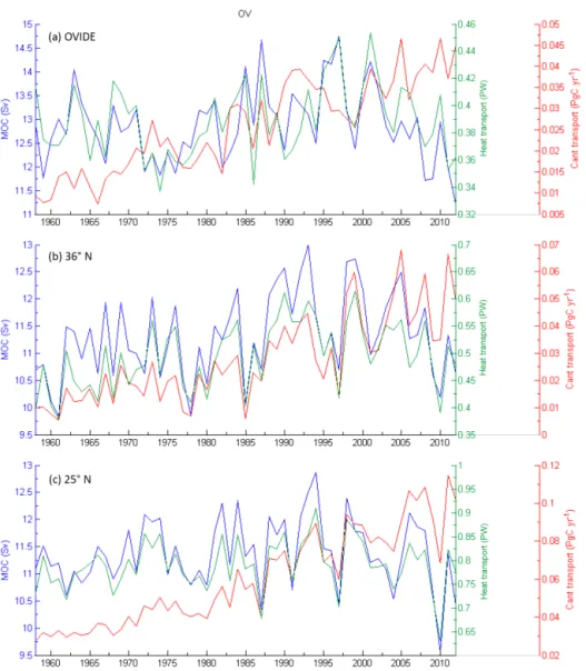
4.1 Controls on interannual to decadal variability of Cant transport
Figure 10 presents annual time series (1958–2012) of the MOC intensity and the transports of heat and Cant across 25◦N, 36◦N and OVIDE. The analysis of annual time series (Table 5a) reveals a strong correlation between the intensity of the MOC and the heat transport across all three sections. Conversely, the transport of Cant only correlates with the MOC intensity at 36◦N. As expected, circulation is the main driver of the interannual to decadal variability of heat trans-ferred across the three sections (Johns et al., 2011; Mercier et al., 2015). Its impact on the Cant transport variability is, however, masked by additional processes.
The transport of Cant across all sections increased con-tinuously over the period of study (Fig. 10, Table 5c). Nei-ther heat transport, nor MOC intensity, nor the net volume of water transported across the sections display a similar in-crease (Table 5c). Zunino et al. (2014) attributed essentially the increase in the northward transport of Cant since 1958 to its accumulation in the northward flow of the MOC upper limb. In order to isolate the circulation effect, we removed the positive trend from the time series of Cant transport. The correlation (r) between the detrended Cant transport and the intensity of the MOC increased from 0.30 to 0.74 at 25◦N and from 0.67 to 0.70 at 36◦N (Table 5a and b). It did, how-ever, not change at the OVIDE section (Table 5a and b). Cir-culation emerges as the dominant control of interannual to decadal variability of Cant transport at 25 and 36◦N, but not across the OVIDE section.
4.2 Interannual to decadal variability of the North Atlantic Cant inventory
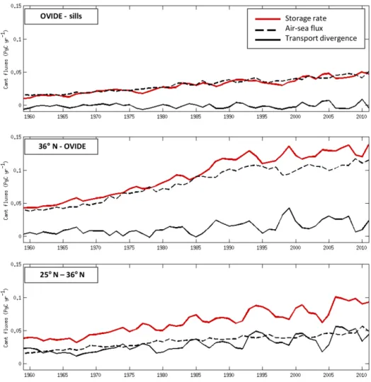
Figure 11 shows the budget of Cant from 1959 to 2011 for the three boxes. Each budget is composed of the storage rate of Cant, the air–sea flux of anthropogenic CO2and the
Figure 10. Annual time series of MOC intensity (Sv), heat transport (PW) and Cant transport (PgC yr−1)simulated by the model at (a) the OVIDE section, (b) 36◦N and (c) 25◦N.
divergence of Cant transport. The storage rate of Cant in-creased continuously over the North Atlantic. The increase was largest in Box 2 (36◦N–OVIDE), where the storage rate
is multiplied by 3, followed by Box 1 (25–36◦N), where it
is doubled. Figure 11 also shows that the air–sea flux of an-thropogenic CO2 and the divergence of Cant transport
con-tributed equally to changes in Cant inventory in the
south-ern box between 1959 and 2011. From 36◦N to the OVIDE
section, the contribution of air–sea flux dominated prior to 1985. From 1985 onward, the transport divergence gained in importance, albeit with a pronounced interannual variabil-ity. In the northern box, changes in Cant inventory followed air–sea fluxes, with a weak contribution of transport diver-gence limited to interannual timescales. The significant posi-tive correlation (Table 6a, no trend removed) between storage rate and air–sea flux in all three boxes suggests that during the past 53 years the latter controlled the Cant storage rate on multi-decadal scales. The transport divergence of Cant
in-creased continuously from 1985 onward in boxes 1 and 2 and is positively correlated with changes in Cant storage rate over 1959–2011 (Table 6a, no trend removed). The Cant trans-port divergence did, however, not contribute to the long-term change in Cant inventory between the OVIDE section and the Greenland–Iceland–Scotland sills (Table 6a), where it is close to zero (incoming TCant=outgoing TCant).
The trend in response to increasing atmospheric CO2
lev-els dominates the signal and the correlation at the expense of interannual variability. In order to identify the controls of interannual variability, the analysis was repeated with de-trended time series. It reveals a strong correlation between the storage rate of Cant and its transport divergence for all three boxes (Table 6b). The correlation with air–sea fluxes is either not significant or weak (Table 6b). The analysis of model outputs suggests that while long-term changes in Cant storage rate are controlled by air–sea flux of anthro-pogenic CO2, its interannual variability is, on the other hand,
Figure 11. Annual time series of contributions to the anthropogenic carbon (Cant) budget (Pg yr−1)simulated by the model (c) between 25 and 36◦N, (b) between 36◦N and the OVIDE section and (a) between the OVIDE section and the Greenland–Iceland–Scotland sills over the period 1959–2011. Contributions are the storage rate of Cant (red line), the air–sea flux of Cant (black dashed line) and the transport divergence of Cant (black full line).
Table 5. Summary of (a–b) the coefficient of correlation (with p value) between the MOC and the transport of heat or Cant at 25◦N, 36◦N and the OVIDE section. The analyses were done first with the original time series (a including trend) and with the detrended time series (b without trend). The trend for each term as well as those of volume transport are reported in the third part of this table (c trend).
25◦N 36◦N OVIDE
(a) Coefficient of correlation (p value) for time series including trend
Theatvs. MOC 0.92 (0.00) 0.90 (0.00) 0.76 (0.00)
TCantvs. MOC 0.30 (0.02) 0.67 (0.00) 0.02 (0.90)
(b) Coefficient of correlation (p value) for detrended time series
TCantvs. MOC 0.74 (0.00) 0.70 (0.00) 0.01 (0.40) (c) Trend TCant(1958–1960) 0.030 ± 0.002 PgC yr−1 0.009 ± 0.001 PgC yr−1 0.008 ± 0.001 PgC yr−1 TCant(2010–2012) 0.095 ± 0.024 PgC yr−1 0.050 ± 0.018 PgC yr−1 0.043 ± 0.005 PgC yr−1 Theat 0.0003 ± 0.0004 PW yr−1 0.0016 ± 0.0004 PW yr−1 0.0003 ± 0.0002 PW yr−1 MOC 0.001 ± 0.005 Sv yr−1 0.016 ± 0.006 Sv yr−1 0.003 ± 0.007 Sv yr−1 Tvol −0.000 ± 0.000 Sv yr−1 0.001 ± 0.001 Sv yr−1 −0.000 ± 0.003 Sv yr−1
Table 6. Correlation coefficient (r) and p value between the time rate of change (Trate) of Cant storage, the divergence of Cant trans-port (DTCant)and air–sea Cant flux (FCant)for the boxes, 25◦N–36◦N, 36◦N–OVIDE and OVIDE–sills, over the period 1959–2011.
DTCant=incoming – outgoing Cant fluxes across the boundaries of boxes. The analyses were done, with the original time series (a with
trend) and with the detrended Cant transport time series (b without trend).
(a) With trend (b) Without trend
Box 25–36◦N Box 25–36◦N
Trate/DTCant:r =0.93, p value = 0.00 Trate/DTCant:r =0.94, p value = 0.00
Trate/FCant:r =0.90, p value = 0.00 Trate/FCant:r =0.04, p value = 0.78
Box 36◦N–OVIDE Box 36◦N–OVIDE
Trate/DTCant:r =0.73, p value = 0.00 Trate/DTCant:r =0.61, p value = 0.00
Trate/FCant:r =0.97, p value = 0.00 Trate/FCant:r =0.52, p value = 0.00
Box OVIDE–sills Box OVIDE–sills
Trate/DTCant:r =0.32, p value = 0.02 Trate/DTCant:r =0.76, p value = 0.00
Trate/FCant:r =0.95, p value = 0.00 Trate/FCant:r =0.22, p value = 0.12
Figure 12. Distribution of volume transport integrated into density (σ1)layers with a 0.3 kg m−3resolution for 25◦N, 36◦N, OVIDE and
the Greenland–Iceland–Scotland sills over the period 1958–2012 (color bar). Dashed lines indicate the density limits of three water classes: Class 1N represents the northward flowing North Atlantic Central Water; Class 1S represents the southward flowing North Atlantic Central Water; Class 2 represents the Intermediate Water; Class 3 represents the North Atlantic Deep Water.
driven by the divergence of Cant transport. Additional anal-yses were made to identify which role is played by the cir-culation in the annual evolution of the storage rate of Cant. For each box, correlations between detrended time series of Cant transport divergence and incoming or outgoing trans-port of Cant were assessed. These estimates, summarized in Table 7, show that the divergence of Cant transport is always correlated with the incoming transport of Cant and not with the outgoing transport of Cant. The interannual variability of the North Atlantic Cant storage rate is thus driven by the transport of Cant coming from the south. The intensity of the MOC controls the interannual variability of both terms
at 25 and 36◦N (Sect. 4.1). The analysis of the full 53-year period corroborates conclusions drawn for the period 2003– 2011 (Sect. 3.3) and is in line with previous studies (Pérez et al., 2013; Zunino et al., 2014).
4.3 Contribution of water masses to the regional Cant
storage rate
In this section, we identify major water masses making up the upper and lower limb of the MOC to evaluate their con-tributions to the regional Cant storage rate over the period 1959–2011. The North Atlantic circulation is well docu-mented. Based on previous studies (e.g., Arhan, 1990;
Mc-Table 7. Correlation coefficient (r) and p value between the di-vergence of Cant transport (DTCant) and the incoming (in) or
outgoing (out) transport of Cant (TCant) for the three boxes,
25—36◦N, 36◦N–OVIDE and OVIDE–sills, over the period 1959– 2011. DTCant=incoming – outgoing Cant fluxes across the
bound-aries of boxes. The linear trend was removed from each times series beforehand.
Box 25–36◦N
inT
Cant/DTCant:r =0.51, p value = 0.00 outT
Cant/DTCant:r = −0.31, p value = 0.03
Box 36◦N–OVIDE
inT
Cant/DTCant:r =0.79, p value = 0.00 outT
Cant/DTCant:r =0.07, p value = 0.62
Box OVIDE–sills
inT
Cant/DTCant:r =0.68, p value = 0.00 outT
Cant/DTCant:r = −0.05, p value = 0.70
Cartney, 1992; Hernández-Guerra et al., 2015; Daniault et al., 2016) and on the vertical distributions of volume trans-ports integrated zonally at 25◦N, 36◦N, OVIDE and the Greenland–Iceland–Scotland sills (Fig. 12), we defined three water classes: North Atlantic Central Water (NACW, Class 1), Intermediate Water (IW; Class 2) and North Atlantic Deep Water (NADW, Class 3).
NACW (Class 1) is transported by upper ocean circula-tion, either northward (Class 1N) by the Gulf Stream and the NAC, or southward (Class 1S) by the subtropical gyre recirculation in the western European basin. The southward recirculation is composed of colder and denser waters (Tal-ley et al., 2008), allowing the distinction of Class 1S from Class 1N in our study (Fig. 12). NACW loses heat during its northward journey, which increases its density. As a result, the density limits between Classes 1N and 1S and 2 change with latitude. Based on Fig. 12, we defined Class 1N from the surface to σ1=29.1 kg m−3at 25◦N, 30 kg m−3at 36◦N
and 31 kg m−3at the OVIDE section. This class is not found at the Greenland–Iceland–Scotland sills. Class 1S, proper to the subtropical region, is found from 29.1 to 31 kg m−3 at 25◦N and from 30 to 31 kg m−3at 36◦N.
IW (Class 2) encompasses the densest water masses of the MOC upper limb, such as Antarctic Intermediate Wa-ter (AAIW), Subantarctic InWa-termediate WaWa-ter (SAIW) or Mediterranean Water (MW). Class 2 circulates northward be-tween σ1=31 and 31.8 kg m−3 from 25◦N to OVIDE and
between σ1=31 and 31.9 kg m−3 through the Greenland–
Iceland–Scotland sills (Fig. 12).
NADW (Class 3) supplies the lower limb of the MOC. It flows southward from the subpolar gyre to the subtropical region. In the model, it is found below σ1=31.7 kg m−3at
25◦N, 36◦N and OVIDE and below σ1=31.9 kg m−3at the
Greenland–Iceland–Scotland sills (Fig. 12).
25° N 36° N OVIDE Sills
(a) 1959–1994
BOX 1 BOX 2 BOX 3
0.029±0.008 0.068±0.022 0.026±0.008 0.003±0.003 0.000±0.000 0.056±0.024 0.012±0.007 0.098±0.024 0.028±0.009 0.022±0.014 0.006±0.005 0.085±0.024 0.004±0.003 0.019±0.005 0.020±0.004 0.076±0.016 0.018±0.004 0.021±0.009 0.011±0.004 0.021±0.004 0.008±0.019 0.013±0.017 0.057±0.020 0.000±0.003 0.006±0.009 0.017±0.011 0.043± 0.010 0.082± 0.035 0.023± 0.008 0.037± 0.009 0.097± 0.028 25° N 36° N OVIDE Sills (b) 1996–2011
BOX 1 BOX 2 BOX 3
0.044±0.005 0.105±0.007 0.042±0.005 0.014±0.008 0.000±0.000 0.105±0.012 0.046±0.024 0.172±0.017 0.050±0.014 0.053±0.018 0.024±0.016 0.141±0.030 0.005±0.003 0.039±0.011 0.032±0.004 0.151±0.017 0.030±0.004 0.036±0.013 0.011±0.008 0.036±0.006 0.016±0.041 0.012±0.043 0.098±0.007 0.001±0.005 0.014±0.015 0.026±0.014 0.079± 0.016 0.095± 0.040 0.039± 0.006 0.087± 0.028 0.175± 0.021
Figure 13. (a) Anthropogenic C budget (PgC yr−1)simulated by the model over the period 1959–1994 for the three water classes and the three boxes (25–36◦N, 36◦N–OVIDE and OVIDE–sills) described in Sect. 4. Horizontal arrows represent the transport of Cant within NACW (Class 1; purple), IW (Class 2; red) and NADW (Class 3; blue) across 25◦N, 36◦N, OVIDE and sills. Grey ver-tical arrows show the air–sea flux of anthropogenic CO2for each
box. Orange values indicate the subregional Cant storage rate. Black vertical arrows represent the derived vertical transport of Cant be-tween classes. The size of horizontal and vertical arrows is pro-portional to the largest Cant flux estimated over the studied period (i.e. 0.098 PgC yr−1of Cant incoming across 25◦N within NACW). (b) Same as Fig. 13a but for the period 1996–2011. To compare with Fig. 13a, note that the size of horizontal and vertical arrows is proportional to the Cant flux incoming across 25◦N within NACW over this period (1996–2011).
Analysis of the long-term changes in the simulated trans-port of volume and Cant across the four sections and for the three specified classes led to identify two periods, before and after 1995 (Fig. S4). The distinction between these two peri-ods is based on Class 1N (northward NACW) at the OVIDE section and Class 2 (IW) at 36◦N for which Cant and vol-ume transports were nearly constant before 1995 but strongly increased after 1995 (Fig. S4). Based on these two periods, the discussion focuses first on 1959–1994 to understand how each water mass contributed to the North Atlantic Cant
stor-Figure 14. Annual time series of the anomaly of volume transport (Sv, bar plot) compared to the winter NAO index over the period 1959–2011 for Class 1 at 36◦N (r = 0.55, p value = 0.00). Winter NAO index was provided by the Climate Analysis Section (Hur-rell and NCAR, https://climatedataguide.ucar.edu/climate-data/ hurrell-north-atlantic-oscillation-nao-index-station-based, last ac-cess: 25 June 2018).
age rate (Fig. 13a). The period 1996–2011 is analyzed next to evaluate the impact of the strong increase in Cant transport after 1995 on the storage rate of Cant.
Before 1995, more than 50 % of Cant transported by
NACW flowing northward (Class 1N) at 25◦N crossed
36◦N, whereas 30 % recirculated southward within Class 1S. At the OVIDE section, the transport of Cant was equal to 12 % of the 25◦N Cant transport, whereas it was close to zero at the sills (Fig. 13a). Figure 13a also reveals positive anthro-pogenic CO2air–sea fluxes for the three boxes as well as a
non-negligible Cant storage rate between 25 and 36◦N. The net transport of Cant within Class 1 was nevertheless positive in all three boxes and higher than the associated Cant storage rate, which suggests a vertical transport of Cant from Class 1 to Class 2. The preceding comment suggests that NACW plays a key role in the Cant storage rate between 25◦N and the OVIDE section, as well as in the transfer of Cant to a lower (denser) layer during its northward transport.
This cross-isopycnal transport between Class 1 and Class 2 (Fig. 13a) causes a decrease in the volume of Class 1 waters and an increase in the volume of Class 2 waters transported northward from 25◦N to the OVIDE section (Fig. S4). This is in line with results from De Boisséson et al. (2012) who highlighted the densification of subtropical central water by winter air–sea cooling and mixing with intermediate waters along the NAC path. Moreover, results from Cant transport (Fig. 13a) also suggest that IW was enriched in Cant be-tween 25◦N and the OVIDE section over the study period. The large Cant uptake north of 36◦N is explained by regional
winter deep convection occurring along the NAC that mixes NACW, rich in Cant, with IW, poor in Cant. It should be noted that the Cant budget of Class 2 in Box 2 has a deficit of 0.01 PgC yr−1. This result suggests that an additional source (e.g., MW, Álvarez et al. 2005) supplies Cant to IW between 36◦N and the OVIDE section.
Figure 13a also shows that 62 % of Cant entering in Box 3 by advection of Class 1 and Class 2 waters and
by air–sea flux was converted into Class 3 inside the box and exported southward. The remainder was stored in Box 3 (18 %) or transported northward through the Greenland– Iceland–Scotland sills as Class 2 waters (19 %). NADW was thus strongly enriched in Cant between the OVIDE section and the Greenland–Iceland–Scotland sills by entrainment of NACW/IW and deep convection, which is in agreement with results from Sarafanov et al. (2012). Finally, a small fraction of Cant entering in Box 2 within Class 3 left the area across 25◦N (24 %, Fig. 13a). The remainder was stored within Class 3 between 36◦N and OVIDE.
After 1995, 27 % of Cant entering within Class 1 at 25◦N flowed northward across the OVIDE section, which is 2 times higher than for the previous period (Fig. 13b). As discussed above, this relative increase in Cant transport at OVIDE was associated with a significant increase in volume transport across the section (Fig. S4a). The latter was multiplied by 1.9 after 1995 at the expense of the diapycnal transport between Class 1 and Class 2 waters, which decreased by 60 % com-pared to the previous period. As a result, less Cant is trans-ferred from NACW to IW. Figure 13b shows that changes in Class 1 waters in Box 2 went along with a relative but small decrease in air–sea flux and in the net Cant transport across 36◦N. In Class 1 of Box 3, the relative increase in Cant trans-port at OVIDE was concomitant with a similar increase in the contribution of the vertical transport of Cant to Class 2 wa-ters as well as with a small decrease in the contribution of air–sea flux. Moreover, the relative increase in Cant trans-ferred into Class 2 (Box 3) is associated with a relative in-crease in Cant transported within Class 2 waters throughout the Nordic sills, in Cant transported vertically into Class 3 waters and in the regional Cant stored inside the box (Class 2 Box 3), but also to a relative decrease in the Cant transport of Class 2 at OVIDE. The excess of NACW rich in Cant enter-ing the northernmost box (OVIDE–sills) was transferred into IW before being exported to the Nordic regions or stored in the subpolar gyre.
5 Discussion and conclusion
The model–data comparison presented here highlights a large underestimation (by 2 or 3 times) of Cant transport by the model, resulting from an underestimation of both vol-ume transport and Cant accumulation in the water column. The underestimation of the NAC and Nordic overflow vol-ume transports was identified as the major model shortcom-ing. It led to an underestimation of the intensity of the up-per and lower MOC. Moreover, the underestimation of the NAC transport resulted in a smaller transport of Cant from the subtropical to the subpolar gyre compared to observa-tions. The missing southward transport of Cant associated with the Nordic overflows resulted in a net transport of Cant to the Arctic region that was closer to observations but for the wrong reasons (Cant transport was 3 times smaller than
Figure 15. Annual time series of the average temperature of the mixed layer for Box 2 (36◦N–OVIDE; red line) and Box 3 (OVIDE–sills; black line) as simulated by the model over the period 1958–2012.
observations at the OVIDE section, while it was only 2 times smaller at the sills). Our analysis also revealed a strong over-estimation of the simulated air–sea flux of anthropogenic CO2 and a total CO2 air–sea flux larger than observations,
especially north of the OVIDE section. North of 40◦N, this overestimation of the total CO2air–sea flux was partially due
to a seasonal cycle dominated by thermodynamics rather than biological activity. The anthropogenic CO2 air–sea flux as
defined in the model (Sect. 2.1) is however not affected by biological activity. The overestimation of the anthropogenic CO2 air–sea flux was thus a response to low Cant
concen-tration in the North Atlantic surface ocean due an underesti-mation of Cant transported to the subpolar gyre (Sect. 3.1). This, in turn, enhanced the air–sea gradient of anthropogenic pCO2. These results are clearly a limit of the model. This is
especially true for the OVIDE–sills box where we observed an unexpected transport divergence close to zero (no contri-bution) along with an overestimation of the anthropogenic CO2air–sea flux.
Compared to the two other terms, the simulated Cant stor-age rate is in line with data-based estimates (Pérez et al., 2013). It reflects the compensation between the underestima-tion of Cant transport and the overestimaunderestima-tion of air–sea gas exchange. However, the spatial distribution of the column in-ventory of Cant is well reproduced by the model, likely due to correct simulation of mechanisms controlling the inter-annual variability of Cant storage rate (Pérez et al. (2013); Zunino et al., 2014, 2015b) despite the underestimation of simulated Cant transport. Having assessed the strengths and limitations of the simulation, we extended the time window of analysis of interannual to multidecadal changes in the North Atlantic Cant storage rate and its driving processes to the period 1959–2011.
Over the last 4 decades, the interannual variability of the simulated Cant storage rate in the North Atlantic Ocean was controlled by the northward transport divergence of Cant. At the OVIDE section, the interannual variability of Cant trans-port was controlled by Cant accumulation in the MOC upper limb, whereas it was also influenced by the MOC intensity at 25 and 36◦N. These results highlight the key role played by the circulation on the North Atlantic Cant storage rate at an interannual timescale since 1958. Additional analysis in
density classes revealed that Cant was essentially stored in
NACW between 25 and 36◦N and in NADW in the
subpo-lar gyre. It also highlighted the key role played by NACW to supply Cant to IW, which was converted into NADW north of the OVIDE section. These water mass conversions are con-sistent with observational studies (Sarafanov et al., 2012; De Boisséson et al., 2012; Pérez et al., 2013). Figure 14 shows that the NAO winter index is correlated with the simulated volume transport of NACW across 36◦N. A positive (nega-tive) anomaly of volume transport is associated with a posi-tive (negaposi-tive) NAO index. This result is in agreement with previous studies reporting an acceleration of the NAC during the transition from a negative to a positive phase (e.g., Dick-son et al., 1996; Curry and McCartney, 2011). This study also addressed the transition between the positive NAO phase of 1980–1990s and the neutral phase of 2000s. The specific pe-riod after 1995 was characterized by a positive anomaly of simulated volume transport of NACW at OVIDE. As shown in Fig. 15, the region between 36◦N and the OVIDE sec-tion underwent a warming of its mixed layer since 1995. The warming found during the transition from a positive (af-ter 1995) to a negative (since 2010) phase is attributed to an increase in the advection of warm and salty subtropical waters into the eastern part of the subpolar gyre (Herbaut and Houssais, 2009; De Boisséson et al., 2012). The analy-sis of model time series suggests that this warming reduces
the volume of NACW converted into IW between 36◦N and
OVIDE (Sect. 4.3 and Fig. S4). More Cant-rich NACW was thus transported northward through the subtropical gyre and across the OVIDE section to the subpolar gyre. This en-hanced northward Cant transport decreased the air–sea gra-dient of anthropogenic pCO2 and slowed down air–sea gas
exchange (Thomas et al., 2008) as observed between 36◦N and the Greenland–Iceland–Scotland sills (Sect. 4.2 and 4.3). Based on Sect. 4.3, this excess of Cant in response to the excess of NACW transported in the OVIDE–sills box was transferred into IW before being stored in the subpolar gyre or exported to the Arctic region.
To conclude, at the multi-decadal timescale, the long-term change in anthropogenic CO2air–sea fluxes over the whole
domain is the main driver of the Cant storage rate in the North Atlantic subpolar gyre. The divergence of Cant
trans-port from 25◦N to the OVIDE section is the main driver on interannual to decadal timescales. Our model analysis sug-gests that assuming unabated emissions of CO2, the storage
rate of Cant in the North Atlantic Subpolar Ocean would in-crease, assuming MOC fluctuations within observed bound-aries. However, in the case of a strong decrease in MOC in response to global warming (IPCC projection 25 %, Collins et al., 2013), the storage rate of Cant might decrease.
Data availability. All references for the availability of in situ data sets are indicated in the text. A simulation of the model data set can be accessed at: https://vesg.ipsl.upmc.fr/thredds/catalog/ ORCA05-ATLN/catalog.html (ORCA05–PISCES, 2018).
Supplement. The supplement related to this article is available online at: https://doi.org/10.5194/bg-15-4661-2018-supplement.
Competing interests. The authors declare that they have no conflict of interest.
Special issue statement. This article is part of the special issue “Progress in quantifying ocean biogeochemistry – in honour of Ernst Maier-Reimer”. It does not belong to a conference.
Acknowledgements. Virginie Racapé was funded through the EU FP7 project CARBOCHANGE (grant 264879). Simulations were made using HPC resources from GENCI-IDRIS (grant x2015010040). We are grateful to Christian Ethé, who largely contributed to obtain Cant transport in the online mode over the period 2003–2011. We want to acknowledge Herlé Mercier (supported by CNRS and the ATLANTOS H2020 project (GA 633211)) and colleagues for leading the OVIDE project (supported by French research institutions IFREMER and CNRS/INSU), as well as Alonso Hernandez-Guerra for the availability of its mass transport data at 24.5◦N. Other data at 24.5◦N used in this paper were collected and made publicly available by the International Global Ship-based Hydrographic Investigations Program (GO-SHIP; http://www.go-ship.org/, last access: 25 June 2018) and the national programs that contribute to it. We are also grateful to two anonymous reviewers for their constructive comments.
Edited by: Arne Winguth
Reviewed by: Two anonymous referees
References
Álvarez, M., Pérez, F. F., Bryden, H., and Ríos, A. F.: Physical and biogeochemical transports structure in the North Atlantic subpolar gyre, J. Geophys Res.-Ocean, 109, https://doi.org/10.1029/2003JC002015, 2004.
Álvarez, M., Pérez, F. F., Shoosmith, D. R., and Bryden, H. L.: Unaccounted role of Mediterranean Water in the
draw-down of anthropogenic carbon, J. Geophys Res.-Ocean, 110, https://doi.org/10.1029/2004JC002633, 2005.
Arhan, M.: The North Atlantic Current and
Subar-tic Intermediate Water, J. Mar. Res., 48, 109–144, https://doi.org/10.1357/002224090784984605, 1990.
Aumont, O. and Bopp, L.: Globalizing results from ocean in situ iron fertilization studies, Global Biogeochem. Cy., 20, https://doi.org/10.1029/2005GB002591, 2006.
Bakker, D. C. E., Pfeil, B., Smith, K., Hankin, S., Olsen, A., Alin, S. R., Cosca, C., Harasawa, S., Kozyr, A., Nojiri, Y., O’Brien, K. M., Schuster, U., Telszewski, M., Tilbrook, B., Wada, C., Akl, J., Barbero, L., Bates, N. R., Boutin, J., Bozec, Y., Cai, W.-J., Castle, R. D., Chavez, F. P., Chen, L., Chierici, M., Cur-rie, K., de Baar, H. J. W., Evans, W., Feely, R. A., Fransson, A., Gao, Z., Hales, B., Hardman-Mountford, N. J., Hoppema, M., Huang, W.-J., Hunt, C. W., Huss, B., Ichikawa, T., Johan-nessen, T., Jones, E. M., Jones, S. D., Jutterström, S., Kitidis, V., Körtzinger, A., Landschützer, P., Lauvset, S. K., Lefèvre, N., Manke, A. B., Mathis, J. T., Merlivat, L., Metzl, N., Murata, A., Newberger, T., Omar, A. M., Ono, T., Park, G.-H., Pater-son, K., Pierrot, D., Ríos, A. F., Sabine, C. L., Saito, S., Salis-bury, J., Sarma, V. V. S. S., Schlitzer, R., Sieger, R., Skjelvan, I., Steinhoff, T., Sullivan, K. F., Sun, H., Sutton, A. J., Suzuki, T., Sweeney, C., Takahashi, T., Tjiputra, J., Tsurushima, N., van Heuven, S. M. A. C., Vandemark, D., Vlahos, P., Wallace, D. W. R., Wanninkhof, R., and Watson, A. J.: An update to the Surface Ocean CO2Atlas (SOCAT version 2), Earth Syst. Sci. Data, 6,
69–90, https://doi.org/10.5194/essd-6-69-2014, 2014.
Barnier, B., Madec, G., Penduff, T., Molines, J. M., Treguier, A. M., Le Sommer, J., Beckmann, A., Biastoch, A., Böning, C., Dengg, J., Derval, C., Durand, E., Gulev, S., Remy, E., Talandier, C., Theetten, S., Maltrud, M., McClean, J., and De Cuevas, B.: Impact of partial steps and momentum advection schemes in a global ocean circulation model at eddy-permitting resolution, Ocean Dynam., 56, 543–567, 2006
Bourgeois, T., Orr, J. C., Resplandy, L., Terhaar, J., Ethé, C., Gehlen, M., and Bopp, L.: Coastal-ocean uptake of anthropogenic carbon, Biogeosciences, 13, 4167–4185, https://doi.org/10.5194/bg-13-4167-2016, 2016.
Brodeau, L., Barnier, B., Treguier, A. M., Penduff, T., and Gulev, S.: An ERA40-based atmospheric forcing for global ocean cir-culation models, Ocean Modell., 31, 88–104, 2010.
Bronselaer, B., Winton, M., Russell, J., Sabine, C. L., and Khati-wala, S.: Agreement of CMIP5 Simulated and Observed Ocean Anthropogenic CO2 Uptake, Geophys. Res. Lett. 44, 12298–
12305, 2017.
Bryden, H. L., Longworth, H. R., and Cunningham, S. A.: Slow-ing of the Atlantic meridional overturnSlow-ing circulation at 25 N, Nature, 438, 655–657, 2005.
Ciais, P., Sabine, C., Bala, G., Bopp, L., Brovkin, V., Canadell, J., Chhabra, A., Defries, R., Galloway, J., Heimann, M., Jones, C., Le Quéré, C., Myneni, R. B., Piao, S., and Thornton, P.: Carbon and other biogeochemical cycles, in: Climate Change 2013: The Physical Science Basis, Contribution of Working Group I to the Fifth Assessment Report of the Intergovernmental Panel on Cli-mate Change, edited by: Stocker, T. F., Qin, D., Plattner, G.-K., Tignor, M., Allen, S. K., Boschung, J., Nauels, A., Xia, Y., Bex, V., and Midgley, P. M., Cambridge University Press, Cambridge, United Kingdom and New York, NY, USA, 2013.