A-Posteriori bounds on linear functionals of coercive 2nd order PDEs using discontinuous Galerkin methods

A-Posteriori Bounds on Linear Functionals of Coercive

2 d

Order PDEs Using Discontinuous Galerkin Methods

by

Joseph S.H. Wong

Submitted to the Department of Mechanical Engineering

in partial fulfillment of the requirements for the degree of

Doctor of Philosophy in Mechanical Engineering

at the

MASSACHUSETTS INSTITUTE OF TECHNOLOGY

Febuary 2006

©

Massachusetts Institute of Technology 2006. All rights reserved.

A uthor ...

.

...

.. .

--.

--'

''Departmr tf

Mechanical Engineering

January 13, 2006

C ertified by ...

...

...

--.

--Jaime Peraire

Professor of Aeronautics and Astronautics

Thesis Supervisor

Certified by ...

Anthony T. Patera

/PrQfessor of Mechanical Engineering

C ertified by ...

...-A

J

David L. Darmofal

Profes

o Aeronautics And Astronautics

Accepted by...

---Lallit Anand

Professor of Mechanical Engineering

Chairman, Department Committee on Graduate Students

MASSACHUSETTS INSTITUTE OF TECHNOLOGY

A-Posteriori Bounds on Linear Functionals of Coercive

"d Order

PDEs Using Discontinuous Galerkin Methods

by

Joseph S.H. Wong

Submitted to the Department of Mechanical Engineering on January 13, 2006, in partial fulfillment of the

requirements for the degree of

Doctor of Philosophy in Mechanical Engineering

Abstract

In this thesis, we extend current capabilities in producing error bounds on the exact linear functionals of linear partial differential equations in a number of ways. Unlike previous approaches, we base our method on the Discontinuous Galerkin finite element method. For equations such as the convection-diffusion equation, the convection term is handled by the standard DG method for hyperbolic problems while the diffusion operator is discretized by the LDG scheme. This choice allows for the effective bounding of outputs associated with high Peclect number problems without resolving all of the details of the solution. In addition to the ability to manage convection dominated problems, we expand the scope of our error bounding algorithm beyond present capabilities to include saddle problems such as the incompressible Stokes equations. Apart from the aforementioned advantages, the DG discretization employed here also produces associated numerical fluxes, which make the complicated "equilibration" procedure that is often necessary in implicit a-posteriori algorithms, unnecessary.

Thesis Supervisor: Jaime Peraire

Acknowledgments

First and formost, I would like to thank my father for his many years of support and en-couragement throughout my academic career, without which this work would not have been possible. In close connection, I wish to convey my gratitude to my former gaurdian, Eugene Wang, who guided my way through my early years in the United States. Obviously, the op-portunities afforded me by my advisor, Professor Peraire, was instrumental to the successes I enjoyed in my doctoral studies. I would especially like to thank members of my doctoral committee, Professors Patera and Darmofal, for their time and guidance. Also critical to the successful completion of this undertaking were the help that Doctors Bethany R. Block, Michelle Massi and Elizabeth Loder provided, whose benefits go far beyond the confines of academic persuit. Finally, I thank all my friends for simply doing what friends do.

Contents

1 Introduction

1.1 Explicit Methods . . . . 1.2 Implicit Methods . . . . 1.3 Proposed Algorithm . . . . 2 Preliminaries and Discontinuous Galerkin Discretization

2.1 Model Problems . . . .

2.1.1 Linear Hyperbolic Equation . . . . . 2.1.2 Poisson Equation . . . . 2.1.3 Convection-Diffusion Equation . . . . 2.2 Domain Decomposition and Function Spaces 2.3 Notation and Operators . . . .

2.4 DG for Linear Hyperbolic Equations . . . .

2.4.1 Discrete Problem . . . . 2.4.2 Convergence . . . . 2.5 DG Discretization for Elliptic Problems: The

2.5.1 Discrete Problem . . . . 2.5.2 A-priori Error Estimate . . . . 2.5.3 Example: Convergence in 2-D . . . .

LDG Algorithm

2.6 DG Implementation for the Convection-Diffusion Equation 2.6.1 Discrete Problem . . . . 11 12 14 15 17 19 19 20 20 21 22 23 24 25 27 30 30 31 31 34

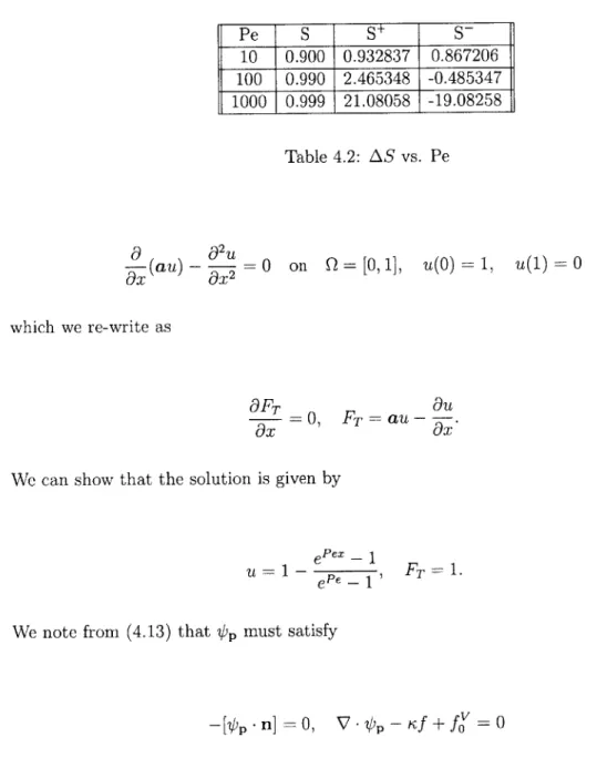
3 Bounds for Linear Functional Outputs: Scalar Symmetric Case . . . . 36 . . . . 36 . . . . 38 . . . . 39 3.1 Problem Definition . . . . 3.2 Lower Bound Formulation: The Lagrangian . . . . 3.2.1 Lower Bound Evaluation: A Simple Example. . 3.2.2 Lower Bound Evaluation: S . . . . . 3.3 Calculation of Lagrange Multipliers: Infinite-Dimensional Case . . . . 3.3.1 Alternative Derivation . . . . 3.4 Calculation of Qu: Finite-Dimensional Case . . . . 3.4.1 Elemental Reconstruction of OpP. . . . . 3.5 Upper Bounds . . . . 3.6 Bound Optimization . . . . 3.7 Error Bound Algorithm Example: Volumetric Outputs . . . 41 . . . 43 . . . 45 . . . 46 . . . 47 . . . 48 . . . 50 53 54 54 4 Bounds for Linear Functional Outputs: Nonsymmetric Case 4.1 Problem Definition . . . . 4.2 Lower Bound: the Lagrangian . . . . 4.3 Calculation of Lagrange Multipliers: Infinite-Dim ensional Case . . . . 4.4 Computation of T': Finite-Dimensional Case . . . . 4.4.1 Elemental Reconstruction . . . . 4.5 Computation of S+, AS and r . . . .. 4.6 Error Bound Algorithm Example: Convection-Diffusion Equation . . . . 4.7 High Peclet Number Problems . . . . 4.7.1 High Peclet Number Algorithm: 1-D Analysis . . . . . 4.7.2 High Peclet Number Algorithm Example: 1-D Case 4.7.3 High Peclet Number Algorithm Example: 2-D Case 4.7.4 High Peclet Number Algorithm Example: 2-D Numerical Example . . . . . . 57 . . . . 60 . . . . 60 . . . . 62 . . . . 63 . . . . 65 . . . . 65 . . . . 68 . . . . 70 71 35

5 Bounds for Linear Functional Outputs: Symmetric Positive- Definite Sys-tems

5.1 LDG Discretization: Plane-Stress Model . . . .

5.2 Energy Balance . . . . 5.3 Lower Bound: the Lagrangian . . . . 5.4 Computation of Lagrange Multipliers:

Infinite-Dim ensional Case . . . . 5.5 Computation of +: Finite-Dimensional Case . . . . 5.5.1 Elemental Reconstruction of ,5y: P1 Case . . . .

5.5.2 Elemental Reconstruction of -: P2 Case . . . .

5.6 Bound Optimization . . . . 5.7 Error Bound Algorithm Example: Plane-Stress

Convergence . . . . 5.8 Error Bound Algorithm Example: Uniformly Loaded Plate

6 _{Bounds for Linear Functional Outputs: Symm} 6.1 LDG Discretization . . . . 6.2 Lower Bound: the Lagrangian . . . .

6.3 Initial Approach . . . .

6.3.1 Energy Balance . . . . 6.4 Proposed Approach . . . . 6.4.1 Energy Balance: Alternative Approach 6.5 Computation of IF: Infinite-Dimensional Case 6.6 Computation of IF: Finite-Dimensional Case

6.6.1 Elemental Reconstruction of -y . . ... 6.6.2 Bound Optimization . . . . 6.7 Stokes Error Bound Example: Channel Flow .

etric Indefinite Systems 99

. . . 100 . . . 104 . . . 105 . . . . 105 . . . . 107 . . . 107 . . . 111 . . . 114 . . . 114 . . . 115 . . . 116

6.8 _{Stokes Error Bound Example: Drag on Square Cylinder . . . .} 7 Conclusion 7.1 _{Contribution . . . .} 75 . . . . 76 . . . . 79 . . . . 8 1 . . . . 84 . . . . 87 . . . . 88 . . . . 89 . . . . 9 1 . . . . 92 . . . . 95 119 123 123

List of Figures

2-1 h = 1/32 Computational Mesh

2-2 h = 1/32 LDG solution . . . . .

h = 1/64 Computational Mesh . . . .

h = 1/64 LDG solution . . . . Problem Setup: Poisson . . . .

h = 1/32 Computational Mesh: Poisson . Primal solution: Poisson, h. . . . .

Dual solution: Poisson, Uh . . . .

Problem Setup: CD1 . . . . Primal solution: CD1, Uh . . . .

Dual solution: CD1, Uh . . . . h = 1/16 primal solution: CD2, Pe=100

h = 1/16 dual solution: CD2, Pe=100 .

2-3

5-9 Deformed Geometry: PS2 . . . . 97

5-10 T 1, Contour: PS2 . . . . 97

5-11 712 Contour: PS2 . . . . 98

5-12 T2 2 Contour: PS2 . . . . 98

6-1 Velocity Vector: Stokesi . . . . 118

6-2 Pressure Contour: Stokesi . . . . 118

6-3 Problem Setup: Stokes2 . . . . 120

6-4 Velocity Vector: Stokes2 . . . . 121

List of Tables

2.2

L2 Errors and Orders of Convergence

L2 Errors and Orders of Convergence 3.1 AS Grid Convergence: Poisson 4.1 AS Grid Convergence: CD1 . 4.2 AS vs. Pe . . . . 4.3 AS vs. Pk, Pe=100 . . . . 4.4 AS vs. Pk, Pe=500 . . . . 4.5 AS vs. le: CD2, Pe=100 . . . . . 4.6 AS vs. le: CD2, Pe=1000 . . . . 5.1 AS Grid Convergence: PSI 5.2 AS Grid Convergence: PS2 6.1

6.2 6.3

Uh, Ph Grid Convergence: Stokesi AS Grid Convergence: Stokes . AS Grid Convergence: Stokes2

27 31 50 65 66 69 69 72 72 95 96 117 117 120

...

. . . .

. . . .

. . . .

Chapter 1

Introduction

Numerical analysis has by now become a standard tool of engineering design. Given a phys-ical problem of interest, an appropriate mathematphys-ical model is formulated and solved by numerical approximation. Indeed, with ever increasing computational resources, the numer-ical solution of mathematnumer-ical problems that were once considered beyond reach are becoming routine. Better algorithms coupled with greater computational capabilities allow the designer to rely ever more heavily on numerical approximations to the solution of detailed mathemat-ical models in engineering analysis. To fully exploit this tool, however, one must be confident that the numerical approximations are delivering solutions of sufficient accuracy. Assuming that the mathematical model describes the physical phenomena of interest adequately, we must ensure that the model is solved with the necessary resolution. A-priori error estimates provide insights concerning the asymptotic convergence behavior of the numerical solution but no guidance as to whether the requisite level of precision has been met by the numerical solution. The analyst is thus left with two choices; to either resort to "overkill" by employing a very fine discretization, which for many problems would result in prohibitive computational costs, or make critical decisions based on unreliable solutions. Clearly, the ability to assess the fidelity of the approximate solution is highly desirable. To this end, various a-posteriori error estimation techniques have been developed to quantify the error in the numerical ap-proximation. Such algorithms fall under two primary categories: 1) explicit error estimators and 2) implicit error estimators. Both approaches can offer important insight concerning the

In general, there are two distinct objectives in a-posteriori error analysis: 1) to obtain local error indicators for use in mesh adaptation and/or increase the asymptotic rate of convergence and 2) to actually produce error bounds on the numerical solution. Explicit methods can fulfill the first objective while the second, more difficult goal usually requires the computationally more expensive implicit algorithms and can only be attained for much more restrictive classes of problems. In addition to differing approaches, a-posteriori error estimation algorithms also differ in the types of error estimates they provide. These algo-rithms produce error estimates for two distinct quantities; the error in some energy or L2

norm of the solution and the error in certain functional outputs that are derived from the solution. We thus have a 2 x 2 matrix of a-posteriori error estimators, from explicit methods for the energy norm to implicit methods for functional outputs.

1.1

Explicit Methods

Given an approximate solution, we would like to extract adaptation and refinement indica-tors that can guide us in converging the numerical solution to the desired level of precision with the least amount of computational effort. Explicit error estimation algorithms can pro-vide precisely that. Finite element analysis has, in fact, long involved explicit a-posteriori error estimation. Inexpensive estimators requiring only local computations were first pro-posed in [7, 6, 8] in the context of continuous Galerkin finite element discretization of elliptic problems. The method provides important insight regarding the quality of the finite ele-ment approximation by attempting to quantify the size of the numerical error in the energy norm. An estimate of the local contribution to the error in the energy norm is produced throughout the computational domain, from which mesh adaptation or refinement strategy may be based. A summary and review of this type of a-posteriori error estimators is given in [2]. The development of similar error estimators for hyperbolic problems has been slower. Nevertheless, the increase in popularity of discontinuous Galerkin methods in recent years has prompted significant research in this area. Work dealing with a-posteriori error analy-sis for nonlinear, hyperbolic conservation laws discretized with discontinuous finite element methods can be found, for example, in [46, 32, 29]. In [16], a-posteriori local L2 error

esti-mates were derived for the Local Discontinuous Galerkin method applied to one-dimensional elliptic problems and in [14] local L2 error estimates were derived for two-dimensional linear

and nonlinear diffusion problems.

In many applications, however, we are less concerned with the size of the numerical error in the energy or L2 norm at a given point in the computational domain than with the error in

certain output functionals derived from the approximate solution. A simple example of this situation is given by airfoil computations; the practitioner is far more likely to be concerned with the error in the calculated values of lift and drag than the error in the L2 norm of any

quantity. An adaptation strategy based on minimizing the error in the energy or L2 norm is

not likely to produce the most efficient means of achieving a given level of precision in the output functionals of interest. This shortcoming has lead to the development of algorithms that produce error estimates on the target functionals of the solution, quantities on which actual engineering decisions will be based. Here, too, the first approaches were devised for elliptic problems solved with continuous Galerkin finite element methods. The first algorithm with such capabilities was proposed in [12], bringing the concept of dual problems and dual

solutions into a-posteriori error analysis, which has since become standard in both explicit

and implicit error estimation. Algorithms based on the same principle include those in [11, 40, 41]. In [28], an algorithm was proposed for producing a-posteriori error estimates on target functionals of the solution of nonlinear hyperbolic conservation laws discretized by discontinuous Galerkin finite element methods. The method also makes use of dual solutions and leads to a significantly more efficient mesh adaptation strategy than one based solely on the local L2 error estimates. More recently, the methodology has been extended to

finite-volume methods in the context of multi-dimensional compressible Euler and Navier-Stokes simulations with turbulence modeling [48, 49, 39]. The primary drawback of explicit error estimators is that while they are very useful tools for mesh adaptation and optimization and applicable to a wide range of problems, these algorithms can provide no guarantees of precision. All explicit error estimates contain generic unknown constants that cannot be evaluated and thus making any guarantee of absolute precision impossible.

1.2

Implicit Methods

To actually obtain absolute error bounds on the numerical solution, one would have to resort to the computationally more complex, implicit methods [1, 33, 9], to which the proposed algorithm also belongs. These methods produce error estimates that do not contain any unknown constants that render them useless as a certification tool, but instead relies on the idea of a "reference" solution. The user first chooses a conservatively refined mesh whose solution is accepted on faith as "exact". These implicit error estimators are then capable of guaranteeing that the energy norm of the discretization error as measured against the reference solution falls within the computed bounds. They are, however, much less generally applicable than the explicit methods cited earlier as they were all developed for linear, self-adjoint problems and provide bounds on only the energy norm. As pointed out earlier, we are rarely interested in the error in the energy norm but rather the error in certain output functionals upon which practical decisions will be based. We also frequently encounter nonlinear problems in practice, which these implicit algorithms cannot treat. Improvements to the cited implicit methods were first introduced in [35, 34, 37] that would allow for the bounding of general linear functional outputs derived from the numerical solution of linear coercive partial differential equations by the traditional Co Galerkin finite element method. The algorithm produces uniform error bounds on linear functional outputs with respect to that of which one would obtain from a reference mesh solution. Treatment of nonlinear and/or non-coercive problems are also possible within this new framework, although in these cases the method produces only asymptotic error bounds on output. It is important to stress that the uniform bounding property of the aforementioned implicit algorithms depends on the selection of a finite-dimensional "reference" solution and that error bounds are only guaranteed with respect to the outputs produced by this finite-dimensional solution and not the infinite-dimensional, exact solution. True certainty thus remains undelivered. Exploiting the complementary energy principle first proposed in the context of error estimation in [26], a further improvement to the implicit approach was made in [30, 43] by removing the need for a finite-dimensional reference solution. The new algorithm is capable of providing uniform error bounds on the linear functional outputs of linear coercive problems with respect to the

exact weak solution of the governing equations. Originally developed for scalar problems

such as the Poisson equations and the advection-diffusion-reaction equation, the algorithm has since been extended to bound the linear functional outputs of multi-dimensional systems such as the governing equations of linear elasticity [36].

1.3

Proposed Algorithm

In the present work, we expand the error bounding capabilities of existing methods in a variety of ways. First, we extend the method put forth in [30, 43, 36] to cover linear func-tionals of linear coercive problems discretized by the Local Discontinuous Galerkin (LDG) algorithm; whose only available a-posteriori error estimates thus far are of the explicit L2

en-ergy type. We then exploit the properties of discontinuous Galerkin discretization to tackle classes of problems that have thus far eluded our grasp; namely, the high Peclet number convection-diffusion equation and saddle problems such as Stokes flow.

One drawback of the algorithm developed in [30, 43, 36] is that when applied to the high Peclet number convection-diffusion equation with under-resolved boundary layers, very poor bounds are produced. This is true even when the output functional of interest is not sensitive to the presence of boundary layers. The problem traces back to the use of the Cauchy-Schwarz inequality and the inability of the algorithm to exploit the orthogonality between error in the primal and dual solutions. By making use of the conservation properties of discontinuous Galerkin discretization, the proposed method alleviates the difficulty presented by under-resolved boundary layers through local refinement of the solution space at the post-processing stage of the algorithm. Effective bounds on linear functionals of the convection-diffusion equations are produced without having to resolve all the details of the solutions in either the primal or dual solutions.

Saddle problems such as Stokes flow also poses significant difficulties for existing methods. Within the framework of the method proposed in [30, 43, 36], the incompressibility constraint makes it near impossible to produce bounds on linear functionals with respect to those calculated from the the exact solution. In the present work, we exploit LDG discretization to define the Lagrangian in such a way so as to not trigger the incompressibility condition in

a manner that would cripple the ability to produce strict error bounds on linear functional outputs. We are thus able to include symmetric-indefinite systems among those whose linear functional outputs we can bound.

One of the most complicated part of implicit error bounding methods is the "Equilibra-tion" step in the algorithm. By using discontinuous Galerkin discretization, we can actually lessen the computational overhead and simplify the error bounding procedure. This is ac-complished by exploiting the numerical fluxes produced by the discontinuous finite element approximation to eliminate the complicated equilibration step that is traditionally necessary in algorithms of this class. The work here may be seen as an extension of the implicit

a-posteriori error bounding algorithm first developed in [35, 34, 37], as the formulation of the

Lagrangian and the expression of the functional of interest as the minimum of a constrained minimization statement remain the same. The work is also in many ways an extension of

LDG discretization as the a-posteriori error bounds are produced for the LDG scheme. The thesis proceeds as follows; in chapter 2 we briefly review the local discontinuous Galerkin method that forms the building block of our algorithm. In chapter 3 we introduce the basic algorithm and apply it to the Poisson equation. In chapter 4 we apply the algorithm to the convection-diffusion equation and develop the necessary modifications to effectively bound outputs associated with high Peclet number problems. Chapter 5 deals with the

application of the proposed method to the equations of linear elasticity. Finally, in chapter 6, we take on saddle problems by applying our method to Stokes flow.

Chapter 2

Preliminaries and Discontinuous

Galerkin Discretization

In this chapter, we examine the Discontinuous Galerkin (DG) discretization for both first order hyperbolic and second order elliptic problems. The discontinuous Galerkin method is a well established technique for the solution of hyperbolic conservation laws, benefitting significantly from the knowledge derived from finite volume schemes. On the other hand, the use of DG methods for the solution of elliptic problems is more recent and several algorithms have been proposed. For the work here, we employ the Local Discontinuous Galerkin scheme developed by Cockburn and Shu [22], which has emerged as one of the most popular DG implementations for elliptic problems (see, for example, [15] for a comparison of various algorithms).

Since its initial introduction by Reed and Hill [42], the discontinuous Galerkin method has gained significant popularity in the computational fluid dynamics community for the numerical solution of hyperbolic conservation laws. The more recent interest in DG methods is sparked by the demand for an algorithm capable of systematically achieving high-order accuracy on arbitrary triangulations of complex geometries while maintaining the ability to handle solution discontinuities.

Traditional finite difference/volume methods enjoy stability and accuracy even in the presence of solution discontinuities such as shocks. This is accomplished by varying the

cedure known as limiting. Generally speaking, these methods involve three distinct steps. First, appropriate numerical fluxes are defined such that when the interpolating polynomial is piecewise constant, the numerical solution is monotonic, guaranteeing stability. Second, a higher-order reconstruction is defined by using linear and higher degree interpolating nomials. In the third step, a nonlinear procedure to limit the slope of the interpolating poly-nomial when in the presence of solution discontinuities is employed to achieve oscillation-free solutions; see [47, 27, 44, 45], for details. These algorithms have been successfully applied to nonlinear conservation laws discretized on structured meshes. On truly unstructured meshes involving complex geometries and boundary conditions, however, high-order reconstruction cannot be easily achieved.

In the finite element framework, on the other hand, high-order accuracy is achieved by using high degree polynomials as interpolating functions within each element and arbitrary triangulations over complicated geometries pose no difficulties in obtaining the desired accu-racy. Unfortunately, traditional Co continuous Galerkin finite element methods lack a natural mechanism to introduce upwinding into the numerical algorithm and thus additional artifi-cial dissipation must be explicitly applied to the numerical scheme. While such algorithms have been developed, they are significantly less robust than finite volume algorithms when applied to nonlinear hyperbolic problems whose solutions contain strong discontinuities.

The discontinuous Galerkin discretization combines the stability of finite volume algo-rithms and the accuracy of classical C' finite element methods, thereby obtaining both accuracy and stability. In addition to exhibiting the same accuracy of classical finite ele-ment discretizations, the DG method also inherits its compact stencil; in direct contrast to high-order finite-volume schemes whose stencil grows with increasing order of approxima-tion. The DG method for hyperbolic problems is uniquely defined once the numerical flux, which introduces upwinding into the algorithm, is chosen. Significant work in the area of DG research has actually evolved around the selection of a suitable interface flux; see for example, [10].

The necessity of treating convection-dominated problems with non-negligible diffusive effects has prompted renewed interest in the extension of the DG concept to elliptic problems in recent years. In the 1970s, a number of interior penalty methods were developed for

discretizing purely elliptic problems with discontinuous or nonconforming elements [3, 4]. Independent of the earlier developments, there are some recent methods designed specifically for treating the elliptic operator in convection-dominated problems which draw on the idea of numerical fluxes traditionally associated with purely hyperbolic equations. A popular method in this class of DG discretizations for elliptic problems is the Local Discontinuous Galerkin (LDG) method introduced in [22] and further studied in [25, 50] and [15]. A review of the available discontinuous Galerkin algorithms for elliptic problems is given in [5].

2.1

Model Problems

In this chapter, we will review the DG discretization for several model problems; namely, the linear hyperbolic equation, the Poisson equation and the convection-diffusion equation.

2.1.1

Linear Hyperbolic Equation

n

V - (au) -

f

a-u = a-g on aQ (2.1)

where u is the solution, g E L2(&Q) is boundary data imposed at inflow, a E !R

2 _{is the}

velocity vector, a± (a -n ± a -nI) and n the outward unit normal; for simplicity, we also assume V - a = 0, which eliminates any coercivity issues that may arise in the underlying

2.1.2

Poisson Equation

n

anD

-V 2u-

f

U = gD on 09D,

Vu

where Q= OQD U aQN, f E L2(Q) is the given forcing and 9D,9N E L2(aQ) are the

imposed Dirichlet and Neumann boundary data, respectively. For discontinuous Galerkin discretization, it is convenient to re-write (2.2) as a system of first order equations

-Vp -

f

u = gD on aQD,

p - n = gN on aQN. (2.3)

where the solution is now u = [u, p]T.

2.1.3

Convection-Diffusion Equation

V. (au - Vu) -

f

with the assumptions that

V a = 0 and a =0

which serves to eliminate any coercivity issues that may arise with the model equation. As is the case with the Poisson equation, we can re-write ( 2.4) as

V (au - p) - f = 0 p - Vu = 0 in _Q, in Q, u = 9D on aQD, Vu .n = 9N on DQN. (2.5)

and look for the solution u = [u, p]T.

2.2

Domain Decomposition and Function Spaces

We consider a partition T of the domain, Q, into Ne non-overlapping subdomains such that

Ne

r =

ZOQ,

\ aQ

j=1

where F is the set of all internal subdomain interfaces. We define the space V and

Q

T _{E X, where}

V {vE L2(Q), V I

E

E

Q

and X = V x

Q.

Vh = {v E L2(Q), V IQ E Pk(Qj),VQj

E T}

Qh {q

E

E

and Pk denotes the space of polynomials of degree k.

2.3

Notation and Operators

Given two adjacent subdomains Q+ and Q- sharing an interface OQ± we define the following interface quantities for an arbitrary scalar valued function v

{ V + [v] = v+n++ vn- (2.9)

2

where n± are the respective outward unit normals to )Ql at an arbitrary point x on ffl. Here v± are the traces of v on (Q'. from the interiors of Q.. For arbitrary vector valued functions q, we define

{q} = + [q - n] = q+ - n+ + q- - n-, [[q]] = q+ 0 n+ + q~ 0 n-. (2.10) 2

As before, q± are the traces q on 9Q'. from the interiors of Q1 and q on denotes the matrix whose ijth entry is qinj. Note that in our definition, [v] is a vector while [q - n] is a scalar.

2.4

DG for Linear Hyperbolic Equations

A description of the discontinuous Galerkin discretization for first-order hyperbolic problems can be found in many references, see for example, [21, 20, 17, 23]. Here, we briefly review it for completeness. After multiplying (2.1) with a test function v E V, integrating by parts over each subdomain Qj and replacing the multi-valued subdomain interface flux with a single valued numerical flux we write

Ne

j

f(-Vv - au - vf)dx + vds

j=1 nj

Oja

+

j

The numerical interface flux, h, is given by

=

a{u}

+

Ia

-n|[u]

}n

(2.12)

where n is the outward unit normal from Qj. We point out that with this definition, full upwind is achieved in the numerical interface flux. In compact notation, we can then write: Find u E V such that

a(v, u) = l(v), Vv E V (2.13)

where a : X x X - R and 1 : X - R are given by

a(v, w) - Vv - awdx + [v] - (a{w}

+

in r 2 fa Q

1(v) j vf dx - j va-gds. (2.15)

Note that this is a variational formulation of the infinite-dimensional continuous problem. We point out that in this formulation, boundary conditions are naturally incorporated into the subdomain interface fluxes; the boundary interface is treated no differently than internal subdomain interfaces with relevant boundary data incorporated into the righthand side of

the equation. From (2.14), we can set w = v to obtain the following expression for a(v, v)

a(v, v) - Vv -avdx + [v - (a{v} + Ja - nI[v])ds +

J

_ --1a - n~v2)ds(2.16)

Sr2 an 2

which after some simplification results in

a(v,v) = Ia-n|[v] 2ds + ja -nv2ds (2.17)

It is clear that for stability we require the a(v, v) to be strictly positive (a(v, v) > 0, Vv), which ensures coercivity. We point out that if we substitute test function v in equation

(2.13) by the exact solution u, we obtain the following energy equality

a(u,u)-l(u) = -jufdx+ 1a -n[u]2ds

+ (

a

",n 2

This expression contains linear and quadratic terms in u, with the latter being strictly positive, a property that we will exploit later on. We note that for the exact solution, u, the interface jump, [u] would be zero.

2.4.1

Discrete Problem

Statement (2.13) together with (2.14) and (2.15) is the point of departure for DG discretiza-tion. We formulate the following discrete problem: Find uh E Vh such that

a(v, uh) = l(v), VV E V (2.19) or Ne 1

_~(-

2.4.2

Convergence

We now examine the convergence behavior of the DG algorithm for linear first-order equa-tions. The order of convergence for the discontinuous Galerkin method for scalar hyperbolic equations for general triangulations was shown in [31] to be of order k + 1/2 in the L2 norm

when polynomials of degree k are used in the numerical approximation. The corresponding

a-priori result is given by

|jejjL2(Q)

: C

for e = u - Uhand constant C_{1 depending on k but independent of u. This result was proven}

to be sharp in [38]; _{however, (2.21) must be seen as a conservative estimate since in practice,}

one routinely obtains order k

+

||eIIL

lal

(2.22)

where again, C2 depends on k but is independent of u.

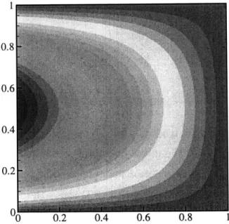
To illustrate this point, we now test the convergence behavior of the DG discretization for linear hyperbolic equations in two dimensions with a simple example. We solve

V-(au)-f= 0 in Q=[0,1]x[0,1]

using P elements with a, = 1, a2 = 0 and f = -aix 2(X2 - 1) such that the exact solution

is u = (1 - Xi)X 2(x2 - 1). The inflow boundary condition is handled weakly through the

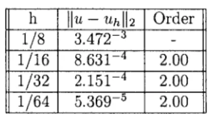
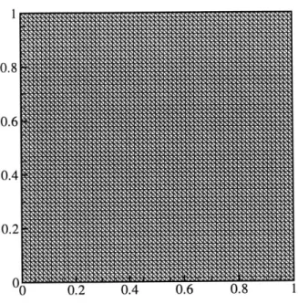
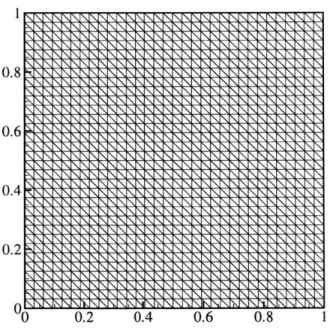
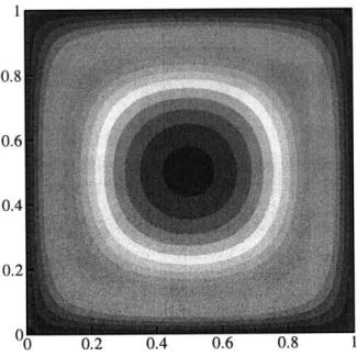
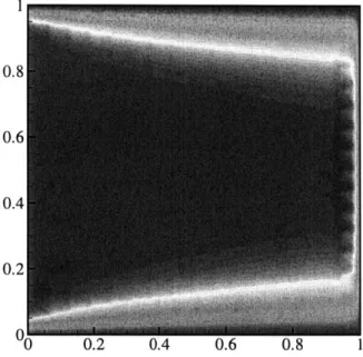
boundary flux. The computational mesh and solution contours for the h = 1/32 computation are shown in figures (2-1) and (2-2). Table (2.1) shows the L2 grid convergence results for

11I

Figure 2-1: h = 1/32 Computational Mesh

1

0.8

0.6

0.4

0.2

0*M _U.2 U.4 U.0 U.6

h

flu

1/8 3.472-3

-1/16 8.631-4 2.00 1/32 2.151-4 2.00

1/64 5.369-5 2.00

Table 2.1: L2 Errors and Orders of Convergence

2.5

DG Discretization for Elliptic Problems: The LDG

Algorithm

We now review the implementation of discontinuous Galerkin discretization for second-order, elliptic problems. As pointed out earlier, there is a plethora of proposed algorithms for the

DG discretization of elliptic equations. For the work here, we have selected the LDG scheme based on its favorable stability and accuracy properties [15, 25]. We consider discretizing the Poisson equation, given by (2.2). The LDG discretization involves first introducing auxiliary variables for the solution gradient and re-writing (2.2) as a system of first-order equations such that we arrive at (2.3). We then multiply (2.3) by arbitrary test functions v E X = V x

Q

inter-subdomain fluxes with appropriate numerical interface fluxes we obtain

N, Vv - p - vfdx - vpds 0 j=1 fq Ne L(q - p + V - qu)dx - Q q nds =0, Vv E X (2.23) j=1

Here

v

j

=({P} + C11 - [U + C12 -[[p]]) n

For stability [22], it is desirable for the matrix

C

C21 C22

to be symmetric and positive definite. This would require C22 to be nonzero and we would lose the ability to eliminate the auxiliary variables p at the elemental level in the resulting dicretized scheme which results in a much more costly algorithm. We therefore only demand

C to be positive semi-definite with C22 set to zero and take it to be

C = C1 C12 (2.26)

-C12 0

with C1 > 0. For interior interfaces, we follow the choice given in [22] and take

0 0 _niCT(.7

C11

Here b is a fixed arbitrary non-zero vector. This choice for / is motivated by the desire to avoid selecting all interface fluxes associated with a given subdomain from the interior trace

(see [25]).

The above choices of numerical fluxes are not always compatible with the imposed bound-ary data at boundbound-ary interfaces. To properly account for the imposed boundbound-ary conditions, we use

3 = {p-a(u - gD)n}. n

U =D

(2.29)

boundary conditions. For Neumann boundaries, we use

P

f = u. (2.30)

In compact notation, we write the following problem statement: Find u E X such that

a(v, u) = 1(v), Vv E X (2.31)

where a: X x X F-+ R and I : X -+ R are given by

a(v, w) =j V -+ q r+V.-qww dx

- [v]

-({r}

C

ir])

+

[q

n]({w}

C

[w[) ds

D v(r - awn) . n ds - q = (2.32)

1(v)

Here v = [v, q]T and w = [w, r]T E X. In the above expression, the boxed quantities are

associated with the conservation law while the double boxed quantities are connected with the definition of the auxiliary variables. Equation (2.31) together with (2.32) and (2.33) defines the variational formulation of the infinite-dimensional problem given in (2.2). From

(2.32), setting w = v results in the following expression for a(v, v)

a(v, v) j Vv. q q V-qvIdx +j av2 ds

[v] - ({q} + C₁₂ [jq]]) + {q- n]({v} -- C₂₁ [v]) ds (2.34)

which after some simplification may be written as

We see that (a(v, v) ;> 0, Vv E X), a result which proves coercivity. We point out for later use that the exact solution satisfies the global energy equality, a(u, u) - I(u) = 0 (obtained form setting v = u in (2.31)). In expanded form, this is given by

j

j

j

j

which again involves linear and quadratic terms in u, with the latter being strictly positive.

2.5.1

Discrete Problem

Statement (2.31) together with (2.32) and (2.33) is the point of departure for LDG dis-cretization. We look for a discrete solution Uh E Xh such that

a(v, Uh) = 1(v), Vv E Xh

(2.37)

E

(q -

jq

-ntds}

This forms a system of equations whose unknowns are Uh and Ph. As pointed out earlier, it is possible with our choice of numerical fluxes, to eliminate Ph locally, at elemental level. This results in a set of equations for Uh whose coefficient matrix is symmetric and positive definite.

2.5.2

A-priori Error Estimate

The LDG algorithm can be shown to converge at order k + 1 for the solution in the L2 norm

and order k for the solution gradient when polynomials of degree k are used in the numerical approximation for general triangulations [22], provided of course, the solution is sufficiently smooth. On cartesian meshes, however, Cockburn proved in [25] that the solution gradient

super-converges at order k + 1/2 in the L2 norm.

2.5.3

Example: Convergence in 2-D

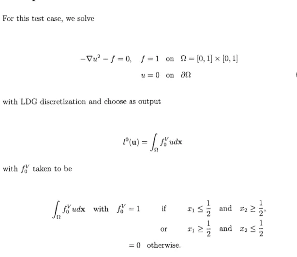
We now examine the convergence behavior of LDG discretization for the 2-dimensional Pois-son equation using piecewise linear elements. For this test case, we solve

-V 2

u -f = 0, f = 0 on Q = [0, 1] x [0, 1]

u (0, y) = u.(1, y) = uY(x, 0) = 0, u(x, 1) = cos(7rX) (2.39)

for which the exact solution is u co"h(7ry) cos(7rx). The computational mesh and the nu-merical solution are shown in figures (2-3) and (2-4) while the grid convergence results are displayed in table (2.2).

h

IJu

IIP

1/8 3.370-3 - 9.993--2

-1/16 8.717-i 1.95 4.918-2 1.02

1/32 2.214-4 1.98 2.445-2 1.01

1/64

5.5775

1.220-2

Table 2.2: L2 Errors and Orders of Convergence

The grid convergence results are in line with the a-priori estimates of order k + 1 and k convergence rate for the L2 norm of the error in the solution and the solution gradient,

respectively.

2.6

DG Implementation for the Convection-Diffusion

Equation

In this section, we review the discontinuous Galerkin method for the convection-diffusion equation. The model problem is given by (2.4). This equation is different from that of the pure diffusion case only in the presence of the convection term, which is easily discretized

1 0 0.6 00000000000000000000000s 0.4 0000000000000000000000, 0.2 0000020000000000000000s 0.2 0.4 0.6 0.8

Figure 2-3: h = 1/64 Computational Mesh

0.8 0. 0.4 0.2 Figure 2-4: h = 1/64 LDG solution I00 0

applying the DG algorithm for first-order, hyperbolic problems to the convection term and the LDG discretization to the diffusion operator. After re-writing the governing equation as a system of first-order equations as shown in (2.5), we multiply (2.5) with arbitrary test functions v and q and integrate by parts over each subdomain Qj. Replacing the multi-valued inter-subdomain fluxes by appropriate numerical interface fluxes leads to

Ne (V - (-au + p) - vf)dx + v(h - P)ds 0 j=1

O

9

The variational continuous problem is then formulated as: Find u E X such that

a(v, u) - l(v) = 0, Vv E X

where a : X x X -* R and 1: XF- R are given by

a(v, w) = V - (-aw + r)I + rV-qw Idx

+ [v] - (a{w} + ja - n[w] - {r} - C12* [[r]]) - [q- n]({w} - C21 w) ds

- v(r-n-aw-a+w) S j q-nwds (2.41)

faOD I SJQN I 1

1(v) = dx

(

+

+

foI

a

As before, boxed quantities are associated with the conservation law while the double boxed quantities are connected with the definition of the auxiliary variables. For the convection-diffusion equation, a(v, v) is given by

We see again, that (a(v, v) > 0, Vv E X); the coercivity condition we need. Globally, we have the following energy equality a(u, u) = 1(u), which becomes

p - pdx + 1la - n[u]ds + (a+ 2 _ a - nu2 + au2)ds uf dx +

r 2 a QD 2

JQD (au + p - n)gDds + JaQN ugNds. (2.44)

2.6.1

Discrete Problem

Statement (2.41) together with (2.41) and (2.42) is the point of departure for LDG dis-cretization. Consider the solution Uh E Xh such that

a(v,uh) = 1(v), Vv E Xh (2.45) or Ne 1

{f(Vv

As is the case with the Poisson equation, the auxiliary variables, Ph, can be eliminated at elemental level. The presence of the convection term, however, means that the set of resulting equations has a non-symmetric coefficient matrix.

Chapter 3

Bounds for Linear Functional

Outputs: Scalar Symmetric Case

In this chapter, we develop the basic framework for the algorithm that produces upper and lower bounds for linear functional outputs of coercive 2nd-order elliptic partial differential equations with respect to the outputs obtained from the exact solution. Unlike [30, 43], however, we base our method on the Local Discontinuous Galerkin scheme, which has the advantage of not requiring the complicated "equilibration" procedure that is necessary in existing implicit a-posteriori error bounding algorithms. The numerical fluxes that are nat-urally produced by the Discontinuous Galerkin discretization to ensure inter-subdomain coupling also serve as "equilibrated" fluxes in the context of implicit error-bounding. The algorithm is in some ways an extension of those presented in [35, 34, 37] as they are both based on formulating the output as the solution to a constrained minimization problem with an augmented Lagrangian. The objective function involves a "quadratic" energy term that derives from the coercivity of the underlying governing partial differential equations plus the linear functional output of interest. The equilibrium governing equations enter as constraints to the minimization. The algorithm may also be seen as an error bounding algorithm for Discontinuous Galerkin methods as it is specifically built for and based on the properties of these schemes.

3.1

Problem Definition

We take as model problem the Poisson equation, given by (2.2). We are interested in ob-taining upper and lower bounds for linear functional outputs of the form

S

j

j

J9

which are functionals of the solution to (2.2). Here,

fev

fo

given functions.

We recall from (2.32) and (2.33) that with the definitions v = [v, q]T, q = [qi, q2, q3]T, u [u, P1T, P = [p, p2P, 3]T, (2.3) may be written in variational form as: Find u E X such that

a(v, u) = 1(v), Vv C X. (3.2)

The output may then be written as S = 10(u) with

10 (v) = vfovdx +

/

Jf2 JaE2D

I8

3.2

Lower Bound Formulation: The Lagrangian

We now proceed to develop the algorithm for the computation of lower bounds for S. As we shall see later on, upper bounds may be obtained in an analogous manner with only a slight modification of the algorithm. Following the methodology of Patera et al. [35, 34], we introduce the Lagrangian, L : X x X -* !R, as

L(v, xL' ) = ,(a(v, v) - l(v)) + 10(v) + a(4', v) - 1(xpv), Vv, xL'

C

where xJ' = [V), 4 j]T and K > 0 is an optimization parameter. We recall from chapter 2 that for the Poisson equation, a(v, v) - l(v) is given by

a(v, v) -1(v) = j (q - q - vf)dx + (av(v- gD)-

q -

- Q VgNds.

(3.5)

where a is a penalization parameter to enforce Dirichlet boundary conditions and that a(u, u) - 1(u) = 0. To refresh our memory, the expression for a(v, w) - (v) is given

by Ne d a(v,w) -l(v) = Vv- rdX - j vds j=1 jf~ + (q -r + V - qw)dx - q - nilds}.

The output, S = l0(u), may then be expressed in terms of the following constrained

mini-mization statement

S =

l(u)

'V).

vEX IvEX

We see this since

sup £(v, 41V)

f

ovEX

00 if a(*v, v) - l(Iv)

$

The maximization over '', forces the minimization over X to select the v that satisfies the

governing equation; the minimizer u. Since a(u, u) - 1(u) = 0 and a(xp', u) - l(xpv) = 0, we

obtain C = 10(u). Furthermore, from duality (see, for example [13]), we can claim that

S = l0(u) = inf sup C(v, 'Pv) = sup inf L(v,

'J)'.

The last equality requires L(v, 'I') to be sufficiently regular, a condition which is satisfied in our case. From the above relations it follows that

S = sup inf L(v, TV) ;> inf L(v, I'), V'' E X.

,vEXVEX vEX (3.9)

We point out that the boxed quantity in equation (3.9) is, in fact, and expression for a lower bound for the output, S. We note that this is true for any ''.

3.2.1

Lower Bound Evaluation: A Simple Example

Before we proceed to derive an expression for the lower bound for S, we digress momentarily to look at the following example. We define a function, Z = Z(y1, y2), given by

Z(yi, y2) = Ay2 + A2y1 + Biy2+ B2 (3.10)

for y = [Y1, Y21T E

R

=

E R

Z*= min Z(yi, y₂)

y1,Y2ER

(3.11)

and obtain the result

4A,

case I - Al +1B2 if A1 >0, B1 =, (312

Z* = _(3.12)

case II - oo otherwise.

From (3.12), we see that when a function is linear and quadratic in its arguments, the unconstrained minimum is either a constant or unbounded from below, depending on the coefficients of its polynomials. This simple problem is, in fact, an analog of (3.9) in that

both Z and C are polynomial functions of their arguments. Here y plays the same role as v in (3.9) while coefficients A, B are the counterparts to x,. The strategy for the remainder of this chapter and in the chapters is then given as follows

1. Define the Lagrangian in a form analogous to (3.12) 2. Choose ''v to ensure that we obtain case I in (3.12)

3.2.2

Lower Bound Evaluation:

S-To evaluate a lower bound for S, we attempt to minimize L over all v = [v, q]T. First,

setting the variation of L with respect to q equal to zero results in

/2

6qdx

= 0 (3.13)

which implies the following constraints

[V1|r

+ go.

and produces the minimizer q = -y;(Vq + V7Pv). Second, setting the variation of L with respect to v equal to zero results in

f (V - - ± f+

)6vdx

* n]ifds

- fj (Oq -n+gN fos)Jvds + ( (2av- 9D) + oz'v )6vds = 0. (3.15)

which requires

V -Vq - rf + foV = 0, [q -

n]lr = 0

We point out that in (3.16), the essential boundary condition on aQD is satisfied in the limit of the penalization parameter, a -- oo. Defining X' as the following subset of X satisfying the following conditions

XC = {IF, E X s.t. [Ov]|r = , [@q -n]|r = 0 V)v IaQD ~K- D + 90, (4'q n) IaN ~KgN + f0 V

q-

+g=0}

We note that in general, the minimization of L in (3.9) over v is unbounded. For %Fv E Xc, however, we do obtain a bounded minimum whose expression is given by (3.19). Here, we make the decision to set a -- oc, as the term contributes negatively to the lower bound,

S. It is then a simple matter to evaluate (3.19) to obtain a lower bound for S. We note

that any ?v, 7q satisfying the conditions stated in (3.17) would produce a lower bound for

the output. Even so, the choice of Ov and 'q plays a critical role in the accuracy of the

computed bounds.

()= - (---( + V/) (4q +

V~) +

4K +

- (V#q - ngD + go)ds ~- V),Nds- (3.19)

3.3

Calculation of Lagrange Multipliers:

Infinite-Dimensional Case

In this section, we develop an algorithm for the computation of the Lagrange multipliers $ and ?/q that will lead to accurate bounds. We will look for Lagrange multipliers V, and V$q in a finite-dimensional subspace of X' C XC c X and we should expect that as X - XC one obtains S-(Tuh) = L(Xu') -> S. The procedure for achieving this involves deriving

optimal values for '', @,u = N)', V)P]T in the infinite-dimensional case; where the bound would be the exact output, and then approximating the resulting expressions discretely.

To this end, we formulate the following constrained maximization problem. We maximize (3.19) with respect to ''. subject to the constraint that xI' E XC

sup inf L*(xv) + Av(V -V@g-

rf

fj)dx

-

4vEX AveX J Jir

- Aq .n(4v + gD - go)ds - Av(V q ' n + K9N - f) ds}

JaD aQN

(3.20)

where A = [A,, Aq]T. We point out that the same Lagrange multiplier, Av, is used to enforce the interface condition of [Vq -n] = 0 and the elemental equilibrium condition. Note that if we choose different multipliers for the boundary and interior conditions, the maximization over @q will force the two multipliers to be the same. Maximizing over 4 q leads to

(- (Op + V/u) -60q + Au6V - V)dx - Au[64q -n]ds -i/D 60q -ngDds -

j

(3.21)