Adding identity to device-free localization systems

Adding Identity to Device-Free Localization Systems

by

Rumen Hristov

Submitted to the Department of Electrical Engineering and Computer

Science

in partial fulfillment of the requirements for the degree of

Masters of Engineering in Electrical Engineering and Computer Science

at the

MASSACHUSETTS INSTITUTE OF TECHNOLOGY

September 2017

c

○ Massachusetts Institute of Technology 2017. All rights reserved.

Author . . . .

Department of Electrical Engineering and Computer Science

August 23, 2017

Certified by . . . .

Dina Katabi

Andrew and Erna Viterbi Professor, MIT CSAIL

Thesis Supervisor

Accepted by . . . .

Christopher Terman

Chairman, Masters of Engineering Thesis Committee

Adding Identity to Device-Free Localization Systems

by

Rumen Hristov

Submitted to the Department of Electrical Engineering and Computer Science on August 23, 2017, in partial fulfillment of the

requirements for the degree of

Masters of Engineering in Electrical Engineering and Computer Science

Abstract

Recent advances in wireless localization systems show that by transmitting a wireless signal and analyzing its reflections, one can localize a person and track her vital signs without any wearables. These systems can localize with high accuracy even when multiple people are present in the environment. However, a primary limitation is that they cannot identify people and know who is the monitored person.

In this thesis, we present a system for identifying people based only on their wireless reflection with high accuracy. We use a semi-supervised learning classifier to assign labels to each person tracked by the device-free localization system. We use recent advances in machine learning to leverage the big amount of unsupervised data that we have. A key challenge that we solve is obtaining labels that are used for guiding the classifier.

To get labeled data, we devised a novel scheme to combine data from a sensor that people are carrying with data from a wireless localization system. We deployed and evaluated our system in people’s homes. We present a case study of how it can be helpful to monitor people’s health more effectively.

Thesis Supervisor: Dina Katabi

Acknowledgments

I am deeply thankful to my advisor, Dina. She changed my way of thinking and helped me focus on the important problems, both in research and in life. She taught me how to be patient when doing research while continuously moving forward and reaching new goals. Seeing her passion and ability to solve challenging problems was my biggest motivation to come to the lab with joy and excitement.

I want to thank Chen-Yu for being an amazing example of a graduate student I should aim to become. He showed me how to solve problems that I thought were impossible to solve. With a smile on my face I think back about the endless hours we spent debugging our system and the time we spent discussing and challenging each other’s ideas. Without him this project would not be possible.

Again, I am thankful to Dina for finding the most hardworking and dedicated group of people I have ever seen. It was a real pleasure for me to work with all of her students. I want to thank Zach for teaching me the basics of hardware and signals and before all being an amazing friend and a great person. I also want to thank Shichao, Mingmin, Ezz, Deepak, Anubhav and Omid for the insightful comments and exciting discussions during group meetings.

I would not have done anything without the support of the people outside of the lab. I want to thank all of my friends at MIT and in The Number Six Fraternity. They were there to cheer me up when I had lost motivation and they were there when I needed someone to celebrate with. I am grateful for the support of the fantastic group of friends that carried me through MIT: Victor, Momo, Rayna, Yvi, Rumen, Defne, Mari, Ekin, Anton, Driss, and Jiajia.

Most importantly, I thank my parents - Galya and Hristo. Every day, I see the impact of their education on the decisions that I make. They made me what I am today and I am extremely grateful for that. Their love and support is what keeps me going. They never lost faith in my success and helped me find my limits.

Contents

1 Introduction 13

1.1 Contributions . . . 16

2 Related Work 17 2.1 Identification with RF Signals . . . 17

3 WiID Overview 19 3.1 Sensor Description . . . 19

3.2 System Overview . . . 20

4 Continuous Movement Detection 23 4.1 Device-Free Movement Detection . . . 23

4.2 Data Collection . . . 24

4.3 Accelerometer Movement Detection . . . 24

4.3.1 Current Limitations . . . 24

4.3.2 Movement Detection . . . 26

4.3.3 Data Augmentation . . . 27

5 Obtaining Groundtruth Labels 29 5.1 Trajectory Preprocessing . . . 29

5.2 Avoiding Data Bias . . . 31

5.3 Acceleration Preprocessing . . . 31

6 Label Expansion 37 6.1 Generative Modeling . . . 37 6.2 Variational Autoencoders . . . 38 6.3 Semi-Supervised Learning . . . 39 6.4 Model Design . . . 41 7 Results 43 7.1 Experimental Setup . . . 43 7.2 Movement Detection . . . 43 7.3 Groundtruth Labels . . . 45 7.4 Label Expansion . . . 46 7.5 Case Study . . . 48 8 Future Work 53 9 Conclusion 55

List of Figures

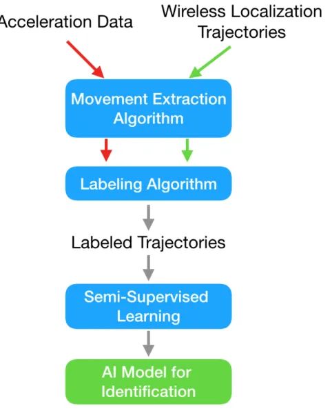
3-1 System Overview. The figure shows a high level overview of WiID. The system combines two streams of data to get labeled trajectories and create an AI model for identification. First, it processes the raw data and extracts the movement of the people. After that, it combines the two streams in order to get labeled trajectories. Finally, these labeled trajectories are used to train a semi-supervised learning classifier. 21

3-2 Label Inference. Once we have trained the model for labeling trajec-tories, WiID can identify people without having them carry any sensors with them. . . 22

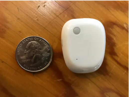
4-1 Metawear. The accelerometer sensor that we used. It is slightly bigger than a quarter. It can easily be carried in the pocket, on a clip on the belt or on a strap around the ankle. . . 25

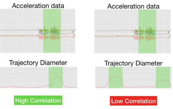
5-1 Trajectory Labeling. On the top we see data from the accelerome-ter. On the bottom there are two different trajectories and their corre-sponding diameters as described in Chapter 4. With green shadow we denote the extracted movement periods. For the plots on the left there is a very high correlation between the two movement periods. Visually it looks like the trajectory belongs to the person carrying this acceler-ation sensor. For the plots on the right, there is a very low correlacceler-ation, so we can deduce that there are two different people. . . 33

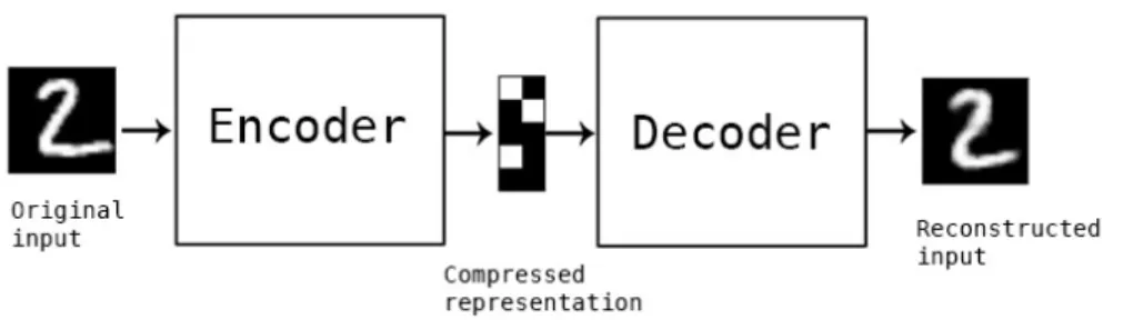
6-1 Autoencoder. The figure shows an architecture of a traditional au-toencoder. There are two main components - an encoder and decoder. The encoder takes the original input and converts it to a compressed representation. The decoder takes a compressed representation as an input and reconstructs the original input of the encoder. . . 39

6-2 Semi-Supervised Deep Generative Models. A graphical repre-sentation of the architecture of our semi-supervised learning classifier. Q is classifying an input into a class 𝑦 and generating latent represen-tation 𝑧, while P is reconstructing the original input from the class and the latent representation. . . 40

6-3 An Example Trajectory. . . 41

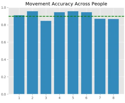
7-1 Movement Accuracy Across People. The average accuracy of the movement detection is 90.08%. The figure shows the results from the 8 different people who did experiments in the lab. We achieve similar to the average accuracy for all of the test subjects. The dashed line represent the average across all people. . . 44

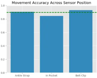
7-2 Movement Accuracy Across Sensor Locations. Our classifier works accurately across all sensor locations. The figure shows that we achieve similar performance on all three positions. . . 45

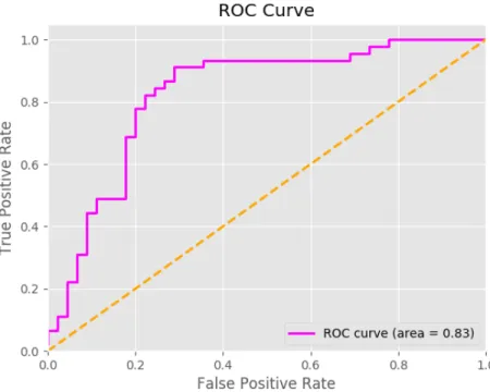
7-3 ROC Curve. The figure shows the ROC curve for the VAE + Semi-Supervised model. The area under the curve is 0.83. If we allow for around 30% false positive ratio, we can get true positive rate close to 100%. If we want to have high precision, we can get around 50% recall for the trajectories of the person with around 10% false positive ratio. 47

7-4 All Trajectories. The home is occupied by multiple people and each of them can generate trajectories and gait measurements. . . 48

7-5 Tagged Subject’s Trajectories. . . 49

7-6 Trajectories With Over 80% Probability Belonging To The Subject. . . 50

7-7 Trajectories With Over 60% Probability Belonging To the Subject. . . 50 7-8 Gait Distribution Tagged as Another Person . . . 51

List of Tables

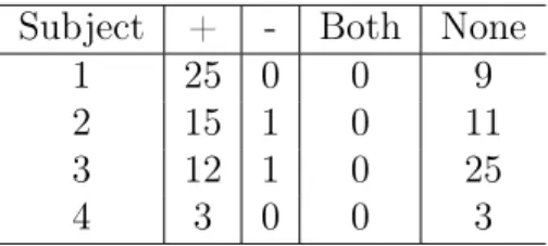
7.1 Classified Trajectories. We show the number of trajectories that got classified with each label for each different person. Subject 1 generated 34 trajectories and 25 of them got tagged with + - our algorithm was confident that this was him, while for 9 of them it didn’t have enough confidence. The total number of trajectories in this period of time is 338. . . 46 7.2 Label Expansion Evaluation. We evaluated the three models and

show the accuracy, precision, recall and F1 score for each of them. The F1 Score is a metric that combines the precision and recall into one. . 47

Chapter 1

Introduction

In-home monitoring of the activities of daily living (ADLs) and detection of deviations from existing patterns is crucial to assessing the health status of elderly people[9, 13]. Real time monitoring can also provide early warning signs about critical events such as falls or hospitalization. In addition to ADLs, gait velocity, frequency of bathroom usage and pacing are valuable metrics for wide range of diseases. The severity of patients with Parkinson’s and Alzheimer’s is directly related to their mobility[19]. Right now, people fill diaries to describe their condition, which is inconvenient and inaccurate[11]. If we can effectively measure mobility metrics at home, we can provide better care for the people.

Currently there is no effective way to measure these metrics at home. One ap-proach that people have tried is to place sensors[8]. One can put an accelerometer on appliances to determine whether they are being used or place sensors on doors to de-termine whether people pass through them. However, this is expensive, inconvenient and not guaranteed to be effective. Another solution is to have the elderly people carry sensors, such as smartphones, to get an estimate of their motion. Unfortunately, the elderly often do not use such devices. Also they are prone to forgetting to carry the wearables with them. There is past work that has used cameras to monitor people at home, but this is highly invasive and unacceptable for majority of the people.

Recently, the emergence of RF-based localization systems have enabled us to ac-curately track the motion of a person without having the user carry or wear any

sensor[4, 3, 24, 23, 20]. These systems can successfully track the location of multiple people in the home and determine whether they are cooking in the kitchen, walking in the hallway or sleeping in the bed.

However, a primary limitation of these device-free localization systems is that they do not know the identity of the people. Systems like WiTrack[4] can successfully track multiple people in the environment, but they have no mechanisms of differentiating between each of the people. They can successfully monitor gait velocity, bathroom usage and general mobility, but without knowing the identity of the person being monitored they are ineffective. Even if the home is occupied by a single person, his visitors will skew the results and may create an impression that the elderly person’s heath status has changed.

We propose WiID, a system that can track multiple people in home and differenti-ate between each of them, without having them carry any sensors on their body. Our system takes as input trajectories of a person from a RF-based localization system and assigns identity labels to each of them. WiID leverages the fact that people have intrinsic habits, which can be used to identify them with device-free localization. For example, people often have their own side of the bed on which they sleep, they take different paths in their homes or have areas where they spend more time than other occupants of the home. Our system learns these habits and distinct characteristics of the person and later can distinguish between the monitored people.

How can we learn the identifying characteristics of a person if they live with multiple other people with which they share a common space and have similar daily patterns? We can ask the person who we want to monitor about what are the different activities they perform or whether they use the space in a different way. However, this is hard for the person and is likely ineffective. We can put cameras inside the person’s home and search for identifying patterns, but this approach is invasive, especially because we want to cover the entire home, including the bedroom and bathroom.

We use a data-driven approach to automatically capture the intrinsic movement characteristics of the people. WiID extracts representative features of the trajectories in an unsupervised way using machine learning. We input the trajectories from the

wireless localization system and find how they are different from each other. We learn in an unsupervised fashion what the most important characteristics of a trajectory are. For example, we can learn that for some homes there is a big variability in the time spent in a given location or that there is a difference of the path people take from the bathroom to the kitchen.

These extracted features help us to classify trajectories. However, in order to do any form of classification, we need to obtain labeled data from people’s homes.

A key challenge that we solve is obtaining ground truth labels at home. We need identity labels for each person tracked by the device-free localization system. Also, we need labels from all the different activities that the person performs during the day and from all the locations at the home. If we do not have labels from the bedroom, for example, then we cannot learn anything about the habits of the person there and later identify him in that area.

Our solution is to provide people with accelerometer sensors that they constantly carry for several days. During this time, WiID correlates the motion from the device-free localization system with the walking periods of the accelerometers that people carry on their body. We developed an algorithm to combine the information from both data streams in order to get both the location of the person and their identity.

We deployed our system with 10 people in 6 different environments. People wore the sensors in their pocket, clipped to their belt or on a strap around their ankle for a period between 7 and 15 days. None of the people complained about the burden of carrying the sensor and were welcoming when asked to carry it for short periods of time. We evaluated our algorithm for tagging location with identity using cameras. In order to verify the classifying algorithm, we split our labeled dataset. Half of we used as a training set, which we gave to the algorithm and half we used as a testing set which we used to evaluate the accuracy of the machine learning algorithm. Our tagging algorithm achieves very high precision, while our classifier achieves 80% accuracy.

1.1

Contributions

To our knowledge, WiID is the first system to continuously differentiate between mul-tiple people moving in an unconstrained way solely based on their wireless reflections. Given a trajectory from a RF-based localization system, we can assign identity to it with high accuracy without having the person carry any sensors on their body.

We extracted intrinsic characteristics of people’s motion in a data-driven way. We developed a novel way to obtain ground truth identity at people’s homes for continuous periods of time. We evaluated WiID in 5 homes and an office space to show that it is highly accurate. This enabled us to monitor the health status of the elderly effectively. We show that by using WiID we can get more accurate measurement of the distribution of the gait velocity of an elderly person at home. This can be used to more accurately track people’s disease progression and general health.

Chapter 2

Related Work

2.1

Identification with RF Signals

Past work has tried to identify people from wireless signals. Some approaches like RF-Capture[2] manage to distinguish between two people with accuracy over 98%. However, RF-Capture requires people to walk on a straight line facing the device. This puts a big limitation on the number of trajectories that can be classified and it cannot be effectively used at home.

Another approach is systems like Hoble[16], WifiU[21] or FreeSense[22]. These systems can distinguish between people based on their gait. However, these systems create signatures using Channel State Information(CSI). However, any change in the environment will modify the CSI and thus the person will generate a different than the recorded signature. If a user at home moves some piece of furniture, the signatures will be changed and the system will stop working.

These systems also require the user to walk on a predefined path or in a very constrained environment. In contrast, WiID works independently on the path that the person walks.

Chapter 3

WiID Overview

3.1

Sensor Description

WiID uses the output of an existing RF-based localization system. It can work with any sensor that localizes people accurately with wireless signals. In particular, WiID uses WiTrack[3] to monitor the environment, but introduces a system built on top of WiTrack to accurately identify the tracked people.

WiTrack[3] is a device that localizes the people in the environment only based on the way they reflect wireless signals. It can track multiple people in the same time and has a range of around 10-12 meters. Its output are trajectories of the people. Each trajectory consists of a set of 𝑥, 𝑦, 𝑡 tuples, where 𝑥, 𝑦 represents the location of a person and 𝑡 is a timestamp. Note that each trajectory is continuous in time, i.e. we can see how a person moved through time. However, we do not know who that person was. We also do not know whether two trajectories were generated from the same person or two different people.

RF-based localization works by detecting motion. If a person is fully static, the device can still detect her from the motion of her breathing, but it has a much smaller signal-to-noise ratio[5]. Environmental noise and multi-path problems can also introduce additional error in the measurements. Our system is designed to be robust against these problems as explained in Section 5.1.

3.2

System Overview

A general system overview is shown in Figure 3 − 1. WiID first combines two data streams in order to obtain labeled trajectories. Using these labeled trajectories, we create a machine learning model to identify people. Later, this model can take trajec-tories from a RF-based localization system and identify the people, without the users having to carry any sensors with them. There are three components which enable us to create a model for identification:

∙ Movement Extraction Algorithm: Our system correlates data from an accelerometer, which the person is carrying, and trajectory data. The first processing step for both data streams is to extract periods when the people are walking. We discuss the challenges and algorithms in more details in Chapter 4.

∙ Labeling Algorithm: This step combines the data from both sensors. We use the location from the device-free localization system and the identity from the acceleration sensors. We devise an algorithm to label trajectories with identity with high accuracy. To achieve this accuracy, WiID implements an important preprocessing step for the trajectories.

Currently, tracking errors related to identity are often disregarded in wireless localization. However, for our system it is critical that a trajectory to be asso-ciated with exactly one person. Chapter 5 goes into greater detail of about the problem and our solution.

∙ Semi-Supervised Learning: WiID captures intrinsic characteristics to the person’s movement in order to be able to identify her without any sensors on her body. Using the acceleration sensor, we can collect highly accurate labels for some of the trajectories. We used these labeled trajectories as an input for a classifier. However, we have little labeled data, because each person wears the sensors for a limited amount of time. To cope with this issue, we first do purely unsupervised learning.

Figure 3-1: System Overview. The figure shows a high level overview of WiID. The system combines two streams of data to get labeled trajectories and create an AI model for identification. First, it processes the raw data and extracts the movement of the people. After that, it combines the two streams in order to get labeled trajec-tories. Finally, these labeled trajectories are used to train a semi-supervised learning classifier.

We use a Variational Autoencoder[15] to extract representative features from the trajectories. An example of these features can be the velocity of the person, the space usage, the time spend in given areas or the way of walking. VAE can extract these features in a completely unsupervised manner by taking as input only the raw 𝑥, 𝑦, 𝑡. This greatly reduces the dimensions of our input and makes

it easier to use the labels and train a classifier.

After we convert the trajectories to a lower dimensional space, we train a clas-sifier. We use a generative model similar to VAE[14]. This model is trying to infer the labels and in the same time it is trying to separate which information of the trajectory is important to its inherit structure. For example, the model can capture that for a given trajectory, it is important to look at the speed in order to infer the label. For another trajectory the label may be more easily inferred based on the time spent in a given area. The algorithm described in [14] is capable for modeling this structure.

Figure 3-2: Label Inference. Once we have trained the model for labeling trajec-tories, WiID can identify people without having them carry any sensors with them.

After the training phase, we create an AI model for inferring the labels. WiID takes as input trajectories from a wireless localization systems and can output a label for each of them with very high accuracy (Figure 3-2).

Chapter 4

Continuous Movement Detection

4.1

Device-Free Movement Detection

As discussed in Chapter 3, we correlate the walking periods extracted from the ac-celerometer sensor with the motion from the device-free localization system. WiID takes as input a person’s location data over time. Then, we identify periods when the person was moving. We cannot simply take the velocity of the person, because the RF-based sensor registers any motion as movement. For example, a person waving his hands while sitting on the couch can be registered as a high speed motion. We use the diameter computation algorithm described in [12] to compute a metric indicative of the actual movement of the person. This provides a more robust metric of moving which does not suffer from the described problems.

We classify every 10-second period as either moving or not. In each period, we consider the 𝑥, 𝑦 locations of the person. We smooth the trajectory with a Gaussian filter so that we reduce the noise and error from the RF-localization system. The algorithm described in [12] efficiently approximates the diameter of the minimum circle that covers all of the points in this 10-second period. We define the person as moving for this period if that diameter is more than 1.3 meters. We chose a threshold that is lower than in [12], because we want to be more sensitive to motion. This allows us to be more precise when correlating both data streams. We could not choose a lower threshold, because it may be exceeded by a semi-static person, who is moving

in place. The localization system would detect his motion with some added error so the algorithm would output that the person is moving.

We chose a 10-second period instead of a shorter one to account for very slow walking. In some of our experiments, the subjects were people with severe form of Parkinson’s Disease. We found out that their natural speed at home is very slow. A 10-second period with a minimum diameter of 1.3 meters guarantees us that we capture all speeds above 0.13𝑚/𝑠, which was low enough for these people.

4.2

Data Collection

We use MetaWear[1] sensors (Figure 4-1) in order to collect acceleration data. The sensor contains an accelerometer and a bluetooth low energy (BLE) chip. It has a very small size of 1 × 1 × 0.5 inches. We asked our subjects to carry the sensors in their pocket, clip it to their pants or carry it on a strap around their ankle. We did not constrain them in any other way and we allowed them to change the location of the sensor throughout the data collection process.

The accelerometer sensor was streaming data via BLE to the RF-based localization device which was already deployed in the subjects’ homes. The range of BLE is similar to the range of RF localization (10-15 meters in a small home), so that we could collect acceleration data while the users were tracked by the device-free localization system. However, existing localization systems have limited range of view and are usually one-directional. Thus, a person could often be in the range of BLE, but not localized by the RF system. This creates challenges which we discuss in Chapter 5.

4.3

Accelerometer Movement Detection

4.3.1

Current Limitations

There is a lot of past work on activity recognition and walking detection from ac-celerometers [18, 17, 10]. However, most of the work has been towards identifying longer walking periods in order to determine daily step count. Another limitation of

Figure 4-1: Metawear. The accelerometer sensor that we used. It is slightly bigger than a quarter. It can easily be carried in the pocket, on a clip on the belt or on a strap around the ankle.

past work is that most of the collected data is in a constrained environment[17]. The test subjects were often asked to walk on a straight line or to perform a specific set of activities which were later labeled from a video recording. It is very challenging to collect labeled data at home. One would need multiple video cameras to cover all of the rooms, while invading the subject’s privacy.

Another challenge comes from the nature of homes and the activities performed inside them. Homes have limited space for walking. Often people take just a couple of steps before stopping again. For example, while cooking a person may use the oven and then make two steps to get to the sink. It is not clear whether we need to label these two short steps as walking or not. This makes the nature of the problem of walking detection ill-defined.

4.3.2

Movement Detection

Our goal is to compare the motion from the accelerometer sensor with the motion observed from the RF sensor. In a similar fashion as in Section 4.1 we focus on every 10-second period. However, we do not classify each segment as walking or not and matching the definition of walking of the RF-based localization. We showed in an example above, how we may want to capture some steps and movement as walking and want to disregard other types of motion.

We use a data-driven approach to solve this problem. We note that our goal is not to extract the raw walking periods from the acceleration. We want to extract the same movement that we extracted from the trajectories. We treat the movement periods from the wireless systems as labels and we train a classifier which tries to extract the same periods from the acceleration data.

We introduce a novel way of collecting labeled activity data at home. Using the RF-based localization system and the algorithm described in Section 4.1, we can mark segments of trajectory data as either moving or not. In the case of a single person in the environment, we can leverage the device-free localization to create labels for the acceleration data. We asked subjects to carry the accelerometer sensor at home for several days, while they made sure they were the only person tracked by the localization system.

We used the acceleration data as an input to a SVM classifier[7] to classify each period as either moving or not. This allowed us to collect days of data in an easy and convenient manner. Also, the data was collected in an unscripted way in an unconstrained environment, instead of it being artificially collected in a lab. Our classifier learned different indicators of movement from acceleration data, instead of only being able to classify walking. Also, the big amount of collected data allowed us to capture movement from all sensor positions(in pocket, clipped on belt or strapped to ankle) with very high accuracy.

4.3.3

Data Augmentation

The accelerometer in the MetaWear sensor has 3 axes. However, we did not require people to carry the sensor in a specific way and it could often change orientation while being carried in the pocket. Thus, we could not leverage any property of the axes. In order to get a better training data distribution, we performed data augmentation by taking all of the permutations of the 3 axes. This allowed us to generalize our training data even more and led to an increase in accuracy.

Chapter 5

Obtaining Groundtruth Labels

WiID combines data from an accelerometer and device-free localization system to assign labels to trajectories. We require very high precision in the assigned labels because we use them as a ground truth for the machine learning module. WiID will only assign a label if it has enough confidence that the trajectory belongs or does not belong to the person being monitored.

We assing labels by looking at the correlation between the data from the ac-celerometer and the trajectories. If there is a high correlation between the moving periods from the two data streams then the trajectory belongs to the person wearing the tag. If there is a little correlation, then this must be another person.

5.1

Trajectory Preprocessing

In order to get high precision in the labeled trajectories, we need to do initial pre-processing. RF-based localization systems have been shown to be highly sensitive and very accurate. They can detect very minuscule motion, but they suffer from bad resolution. They can easily detect movement of limbs as small as hands, but they can have localization error of up to one meter. If there are two people staying close to each other, then the localization system will have a hard time deciding whether a motion between them came from one or the other. An example of a very challenging case for these systems is two people crossing paths. If two people walk in opposite directions

and cross paths, the system will not be sure whether they continued walking in the same direction or whether both of them turned back.

These mistakes do not have a negative impact on the performance of the tracking system on its own, because the trajectories do not usually have assigned identity. However, WiID makes the assumption that each trajectory has a single identity. It is not clear what we should do if a trajectory is identified with two different people because of a mistake. If we label it as belonging to the person that we monitor, we may extract identifying characteristics that do not belong to him. If we label it as not belonging to him, we will lose information and consider his habits as intrinsic to a different person.

To avoid these mistakes we preprocess the trajectories to remove cases of uncer-tainty. We chop them in two when we detect that there is a high chance that there has been an identity switch. However, we would like to do this as little as possible. Maintaining longer trajectories can help us follow the path of the person for a longer time. This would allow us to learn more complicated habits and it will be easier to differentiate between people.

We split the trajectories in the following cases:

∙ Two people are at most 1.5 meter away from each other for more than 3 sec-onds. We empirically chose a distance of 1.5 meters, as this was the maximum separation under which we were observing identity switches.

∙ A person moves by more than 0.5 meters for less than 0.2 seconds. Practically, this implies a speed of 2.5 meters per second, which is rarely observed at homes. The tracking algorithm allows this because it often means just a noisy measure-ment of the localization system. In our observations, we saw that this can also imply that the trajectory switched identity. These big jumps were a sign that the tracking algorithm started tracking another person nearby, who was not yet tracked by the system. In this case, the algorithm was unsure whether there was a noisy measurement or two different people.

system carry the same identity.

5.2

Avoiding Data Bias

WiID captures acceleration data continuously while the person is carrying the ac-celerometer sensor. This guarantees that we capture trajectories everywhere in the home and throughout the whole day. If we did not get labeled trajectories from the bedroom, for example, then we could not learn any of the habits of the person right before going to sleep. This will create a data bias as our labels would be biased towards certain characteristics. For example, our system would not be able to learn on which side of the bed the monitored person sleeps. In this scenario, we would not be able to identify trajectories around the bed, which would limit our capabilities if we want to capture characteristics of the person’s sleep.

Our system labels trajectories only when we are confident in the observation that we make. In the previous example we may not be entirely confident about the identity of the trajectory going to bed. In this case WiID will leave it as unlabeled. However, these events are sporadic. They are independent of the time or the location of the trajectory, but depend on other factors such as system noise and other people in the environment.

WiID identifies trajectories from every location and every time of the day as long as the person is wearing the sensor, but there is some chance of leaving the trajectory unlabeled. This allows our system to generalize very well and learn complicated intrinsic movement characteristic of the person.

5.3

Acceleration Preprocessing

We asked the subjects to carry the accelerometer sensors continuously with them while they are at home. However, the subjects had to take the sensor off while showering and in the periods when they were charging it. This resulted in the sensor being fully static, while still being in the range of the receiving device. If the monitored

person was walking during the period while the sensor was static, there will be very low correlation between the two data streams. Our algorithm would likely label her trajectory incorrectly. This mistake would propagate the wrong label and we would learn incorrect information about the person.

To deal with this issue, we preprocess the acceleration data. People stay static for a long time, but even during sleep they are rarely static for more than an hour. Based on this, we remove periods when the sensor is static for longer than 10 minutes. This is an indicator that there is a high chance that the person may have taken the sensor off. As discussed in Section 5.2, it is better to be more conservative when we label trajectories, as long as we do not introduce data bias.

5.4

Labeling Trajectories

WiID uses an algorithm to label trajectories if it has enough confidence. We extract the movement periods from the acceleration data and the movement periods from the trajectory data. The algorithm looks at the correlation of the two streams. Figure 5-1 shows a simple example of a labeled trajectory. The green shadowed areas indicate the movement periods. We can notice that the two data streams on the left were generated by the same person because the shadowed areas overlap almost perfectly. The streams on the right do not look similar, so they must be generated from different people.

However, looking only on the direct correlation between the two data streams can create wrong labels. An example adversarial situation is the following: the person being monitored is in bed sleeping, but outside of the range of the RF-based system, while another person is sitting on the couch and watching TV. The trajectory of the person sitting on the couch will not have any moving periods, but neither will the acceleration data of the monitored person. There will be perfect correlation between the two streams, but we will assign the label to the wrong trajectory.

Another problem about looking at the direct correlation is that it does not account for error accumulation in the movement detection. We showed in Chapter 4 how we

Figure 5-1: Trajectory Labeling. On the top we see data from the accelerometer. On the bottom there are two different trajectories and their corresponding diameters as described in Chapter 4. With green shadow we denote the extracted movement periods. For the plots on the left there is a very high correlation between the two movement periods. Visually it looks like the trajectory belongs to the person carrying this acceleration sensor. For the plots on the right, there is a very low correlation, so we can deduce that there are two different people.

extract movement periods, but the methods can have slight errors. The example on the left on Figure 5-1 shows how the two green shadows are not perfectly aligned. This is natural, because the two data streams have different errors and slight mis-alignment can always appear. However, if we have a very long trajectory this error will accumulate, but only for the periods when there is a change in the state. One can try to divide by the trajectory length or the number of state transitions, but it is unclear what would be the best threshold.

We propose a simple and efficient method to deal with these problems. Our algorithm can either tag a trajectory with a + or with a −. A + tagged trajectory indicates that there is strong correlation in some period of the trajectory. A − tagged trajectory indicates the opposite - that the is very low correlation in some period. Note that one trajectory can be both + and − tagged. Finally, we assign a positive

identity label (trajectory belongs to the person) iff it is only + tagged and we assign a negative label (trajectory does not belong to the person) iff it is only − tagged.

The tags are assigned with the following two rules:

∙ We assign a + tag if the following conditions are met.

1. For any 12 second period, we have perfect correlation for at least 80% of the time in the extracted movement.

2. For this period, the trajectory is static for at least 30% of the time.

3. For this period, the trajectory is moving for at least 30% of the time.

∙ We assign a − tag if for any 5 second period we have complete disagreement between the data streams.

The time intervals were empirically chosen to account for the accuracy of the movement detection classifier. Often, there is misalignment between the two data streams, but it is often for at most a second or two, thus we require only 80% of the trajectory to be correlated with the acceleration data.

Assigning a + label requires correlation in both static and a moving period. This restriction will solve the problem of mislabeling a person when he is completely static, as discussed above. It will also not allow to mislabel a person, when there are two people continuously walking in the environment. To create a wrong label, multiple people need to walk and stop in the same time, however, this rarely happens in practice.

We assign a − label, if there is strong disagreement. This is a strong indicator that a person in the environment was walking, while the monitored person was static or the opposite. We can deduce that the − labeled trajectory does not belong to the person.

We do not label trajectories tagged with both + and − as negative, because we want to achieve very high accuracy. By not labeling them, we take a conservative approach. A + label indicates a high degree of correlation, which may indicate that such a trajectory may suffer from localization mistake.

This algorithm can be performed very efficiently just by scanning through both data streams in parallel and only looking at the movement periods. The simple rules guarantee us high degree of accuracy for the labeled trajectories. Because of their simplicity, they also allow us to label a lot of trajectories.

In Section 7.3, we present results that show that most of these labels are highly accurate and we have almost perfect precision. We also show that for most of the trajectories of the person that are detected by the RF-based localization system we have enough confidence to assign a positive label.

Chapter 6

Label Expansion

We built a classifier to assign identity labels to trajectories. In order to train the classi-fier we worked with a very small amount of labeled data. WiID uses machine learning techniques such as Generative Modeling and Variational Autoencoder to leverage the big amount of unlabeled data to help the model learn a compact representation of the trajectories.

6.1

Generative Modeling

Generative modeling is a broad area of machine learning which deals with models of distributions 𝑃 (𝑋), defined over data points 𝑋 in some potentially high-dimensional space 𝑋. For instance, images are a popular kind of data for which we might create generative models. Each datapoint (for example, image) has thousands or millions of dimensions (pixels), and the generative model’s job is to somehow capture the depen-dencies between pixels, e.g., that nearby pixels have similar color, and are organized into objects. Exactly what it means to capture these dependencies depends on what we want to do with the model.

One straightforward kind of generative model simply allows us to compute 𝑃 (𝑋) numerically. In the case of images, 𝑋 values which look like real images should get high probability, whereas images that look like random noise should get low probability. However, models like this do not generalize well - knowing that one

image is unlikely does not help us synthesize one that is likely.

We can formalize this setup by saying that we get examples 𝑋 distributed accord-ing to some unknown distribution 𝑃𝑔𝑡(𝑋), and our goal is to learn a model 𝑃 which

we can sample from, such that 𝑃 is as similar as possible to 𝑃𝑔𝑡.

It may not be clear, why a generative model will help WiID to identify people. However, most generative models capture the dependencies between objects in an unsupervised way. If we can reformulate these dependencies into identifiable charac-teristics and have a way to extract them than we will get exactly what we need.

6.2

Variational Autoencoders

A traditional autoencoder takes as input 𝑋 and transfers it into a latent space 𝑧, where 𝑧 has a much lower dimension. A decoder module can transform a latent space state into a reconstructed output. An autoencoder’s goal is to minimize the difference between the reconstructed output and the input. Mathematically it is trying to minimize the following loss function:

𝐿𝑟𝑒𝑐𝑜𝑛𝑠 = 𝐸𝑞(𝑧|𝑥(𝑖)₎(𝑙𝑜𝑔(𝑝(𝑥(𝑖)|𝑧)))

The reconstruction quality is 𝑙𝑜𝑔(1) if the reconstructed output always matches the input.

However, the latent space 𝑧 for an autoencoder does not have any interpretation. A vector 𝑧1 in the latent space can be very similar to vector 𝑧2, but their decoded

outputs may be totally different. If we encode an input into a latent space, we can’t modify the latent variables and expect to get a meaningful output.

One of the most popular generative frameworks is Variational Autoencoder (VAE). They idea is similar to traditional autoencoders, but it ensures that the latent space representation of the input follows a specific structure. There is an added regulariza-tion term in the loss funcregulariza-tion:

Figure 6-1: Autoencoder. The figure shows an architecture of a traditional autoen-coder. There are two main components - an encoder and deautoen-coder. The encoder takes the original input and converts it to a compressed representation. The decoder takes a compressed representation as an input and reconstructs the original input of the encoder.

Where 𝐷𝐾𝐿 is the Kullback-Leibler divergence. This regularization term tries to

bring the distribution of the latent space 𝑧 as close as possible to some distribution 𝑝(𝑧). A common choice of 𝑝(𝑧) is a Gaussian Distribution with mean 0 and standard deviation of 1. This regularization will bring all of the inputs as close as possible in the latent space while still being able to reconstruct well. The combination of the two loss terms will ensure there is balance between reconstruction accuracy and compactness of the latent space.

This structure of 𝑧 can create interesting properties. VAE tends to learn different characteristics of the input distribution for each dimension of the latent variable. For example, if our input 𝑋 is a voice recording one dimension of 𝑧 can learn whether the voice is of a man or woman. Another dimension can learn the pitch or whether the voice has positive or negative connotation.

6.3

Semi-Supervised Learning

WiID uses Variational Autoencoder to learn condensed representation of trajectories. This representation captures the identity of the people and we can train a classifier on top of them.

We can use a standard SVM classifier. However, the amount of labels that we have is very small. We can leverage the big amount of unlabeled data that we have.

We use the unlabeled data to guide the training of the classifier and improve the accuracy.

Figure 6-2 present a graphical representation of the model that we use [14]. In this case 𝑥 is the latent space representation of our input, 𝑄 is the encoder and classifier of the model and 𝑃 is the decoder. Each ℎ is a complex function - in our case it is a neural net.

Figure 6-2: Semi-Supervised Deep Generative Models. A graphical representa-tion of the architecture of our semi-supervised learning classifier. Q is classifying an input into a class 𝑦 and generating latent representation 𝑧, while P is reconstructing the original input from the class and the latent representation.

The model is similar to traditional autoencoder, but with an additional latent variable 𝑦. The first part of the model is taking the input 𝑥 and calculating the probability 𝑝(𝑦|𝑥). After that we use both the label 𝑦 and the input to get the probability 𝑝(𝑧|𝑥, 𝑦). The generative part of the model is trying to reconstruct 𝑥 by using both 𝑦 and 𝑧.

The model is trying to separate characteristics important to the label 𝑦 to general characteristics of the input. In the example of classifying handwritten digits, it will try to separate the label of the digit from it’s writing style. In our problem, we will try to separate the characteristics important to the identity of the person, to the trajectory location and style.

6.4

Model Design

We use a standard semi-supervised generative model. However, we have to make two important design decisions about it. We had to specify representation of the input 𝑥 and to concretely model the components ℎ (Figure 6-2).

As described earlier, our trajectories are a time series data where for each times-tamp we have 𝑥 and 𝑦 coordinates of the person. However, each trajectory has a variable length size and we cannot represent it as a fixed size vector - the usual rep-resentation for an input. Instead of using time series data as input, we project each trajectory on the 𝑥𝑦 plane.

(a) Trajectory on a 𝑥𝑦 plane. (b) Discretized trajectory.

Figure 6-3: An Example Trajectory.

We divide the space that the localization system covers into image consisting of 56 × 56 pixels. This resulted of bins of size around 30cm by 30cm. Each pixel has a value depending on whether the trajectory had a point that falls inside the pixel (Figure 6-3).

However, projecting the trajectory on the 𝑥𝑦 plane loses the temporal information. For example, we do not know which point is the start of the trajectory and which is the end. Thus, our discrete image is not a simple black and white image.

We include time information in each pixel. Starting from the beginning of the trajectory, we assign incrementing numbers to the pixels of the corresponding

coor-dinate. Thus pixels in the beginning of the trajectory will have small values, while pixels around the end will have bigger ones. In the end we normalize the image.

The other decisions in our model was the structure of the function ℎ. We used deep neural networks for each stage of ℎ. In the Variational Autoencoder, which takes as input the raw trajectories, the encoder and decoder use two layer fully connected layers with 500 neurons. In the Semi-Supervised architecture we use a single layer of fully connected network of 300 neurons.

Chapter 7

Results

7.1

Experimental Setup

We implemented WiID using WiTrack[4] and MetaWear[1] sensors. We deployed our system in 5 different homes and 1 office environment. We collected acceleration data from 10 people. In total we have more than 100 days of collected acceleration data.

Each of the people carrying the sensors had 3 options for placing it on their body. Four of them chose to wear it on a strap on their ankle, three of them chose to wear it in their pockets and three of them wore it on a clip on their belt. This shows that different people found different placements more convenient. WiID managed to show high accuracy independent of the sensor placement.

7.2

Movement Detection

The first step of our system is to accurately detect the movement from the accelerom-eter. As explained in 4, we use a SVM classifier to predict whether every segment of acceleration data is walking or not.

We collected labeled data for the classifier in two different ways. We used data from homes with only a single occupant. This guaranteed that every person localized by the device-free system in that home is the one wearing the sensor. This approach provided us with data from the home, where people perform many different activities.

We also collected data from the lab to get movement samples from different people. We asked the subjects to walk, sit and get up multiple time. We also asked them to wear three accelerometers on different body locations so we can collect data from several streams at once.

We collected data from 8 people in the lab where each experiment was 30 minutes long. The subjects ranged from 19 to 67 years old. We recorded multiple days of data from the homes of 2 people.

Figure 7-1: Movement Accuracy Across People. The average accuracy of the movement detection is 90.08%. The figure shows the results from the 8 different people who did experiments in the lab. We achieve similar to the average accuracy for all of the test subjects. The dashed line represent the average across all people.

The overall average accuracy of the movement detection is 90.08%. We evaluate our model by classifying each 10 second period as movement or not. We generated the input data by sliding the 10 second period by 1 second at a time, i.e. the first 10 seconds are the first input, the period from second 1 to second 11 is the second input and so on.

This accuracy may seem low. However, a careful analysis of the errors shows that often our classification has a slight offset with the real data. We often classify one

period as not movement but we classify correctly the next period that starts a second later. This delay is not really important and is an artifact of the way we classify the data into movement or not. We designed the next step (the tagging algorithm) with knowing the specific structure of these errors and set up appropriate parameters for it.

Figure 7-2: Movement Accuracy Across Sensor Locations. Our classifier works accurately across all sensor locations. The figure shows that we achieve similar per-formance on all three positions.

Figures 7-1 and 7-2 show that our accuracy remain high, even across different people and sensor positions.

7.3

Groundtruth Labels

In order to evaluate the labeling algorithm, we used a camera to get the ground truth identity. However, camera is highly intrusive and we performed our experiments only in the office environment as none of our subjects agreed to put a camera in their home.

The office environment is highly active. Twelve people work there daily and several more walk through it on a regular basis. We asked 4 people to carry the acceleration sensors and for each of them we looked at the accuracy of the tagging. Table 7.1 shows the results across subjects.

Subject + - Both None 1 25 0 0 9 2 15 1 0 11 3 12 1 0 25

4 3 0 0 3

Table 7.1: Classified Trajectories. We show the number of trajectories that got classified with each label for each different person. Subject 1 generated 34 trajectories and 25 of them got tagged with + - our algorithm was confident that this was him, while for 9 of them it didn’t have enough confidence. The total number of trajectories in this period of time is 338.

Our algorithm tags each tracklet with one of the 4 labels - +, -, Both, None. The first two indicate a high confidence that the trajectory belongs or does not belong to the person, respectively. The latter indicate that there is contradicting information or no information about this trajectory.

We see that our algorithm has very high precision and rarely labels a tracklet incorrectly with high confidence. The number of tracklets that are tagged with - for each person is between 100 and 142.

On average, our algorithm tags around 50% of the trajectories with a person with high confidence. In the same time, we assign a negative label for 30 to 40% of the trajectories. The combination of these two guarantees that we had enough tagged trajectories to work with when designing the machine learning classifier.

7.4

Label Expansion

We validated the label expansion algorithm by using the labels gathered in the pre-vious step. We got data from 12 days of the person and we used the first 8 days for training, 2 days for validation and 2 days of testing.

As shown in the previous section, most of our labels are negative. In order to fix the issue with heavily imbalanced classes, we make sure that we balance the two classes.

Model Accuracy Precision Recall F1 Score SVM 0.6 0.35 0.69 0.46 VAE + SVM 0.74 0.86 0.69 0.76 VAE + Semi-Supervised 0.78 0.73 0.91 0.81

Table 7.2: Label Expansion Evaluation. We evaluated the three models and show the accuracy, precision, recall and F1 score for each of them. The F1 Score is a metric that combines the precision and recall into one.

𝑥𝑦 plane. In our experiments we used a space of 10 by 10 meters and image of size 56 by 56. This discretized the space in pixels which are around 17 by 17 centimeters.

We compare 3 classifiers: a baseline SVM classifier, which takes as input the raw image. An SVM, which takes as an input the latent representation from the Variational Autoencoder and a Semi-Supervised generative model (as described in Section 6.3). Table 7.2 shows the results for the different models.

Figure 7-3: ROC Curve. The figure shows the ROC curve for the VAE + Semi-Supervised model. The area under the curve is 0.83. If we allow for around 30% false positive ratio, we can get true positive rate close to 100%. If we want to have high precision, we can get around 50% recall for the trajectories of the person with around 10% false positive ratio.

Our results show that WiID can identify people with 0.78% accuracy without them carrying any sensors on their body. We also get high precision and recall results and a F1 score of 0.81.

Simply giving the raw image does not lead to good results as the input dimension is very large and the SVM cannot easily model the training data.

7.5

Case Study

One of the subjects with who we conducted experiment was a patient diagnosed with a mobility disorder. We deployed WiTrack with the patient and wanted to monitor the gait velocity. However, the patient does not live alone, but shares the home with multiple other people. We monitored the gait over time using the algorithm described in [12]. Figure 7-7a shows the distribution of the gait measurements that we collected over a period of 12 days. In this figure, each gait measurement can be from any of the occupants of the house.

We also visualize the trajectories that are generated by WiTrack in the same period of time on a 𝑥𝑦 plane. Figure 7-7b shows them all plotted on top of each other. The green rectangle on top of the plot is the device. We can see that they span several room of the home and we can see the coverage of the device.

(a) Gait Distribution (b) Trajectories projected on 𝑥𝑦 plane

Figure 7-4: All Trajectories. The home is occupied by multiple people and each of them can generate trajectories and gait measurements.

The gait velocity of the patient as measured in clinic is around 0.3 meters per second as the patient has problems with mobility and uses a walker. From this distribution, we cannot differentiate between the monitored person’s walking and the walking of the others and we cannot make conclusions about the patient’s health.

After we asked our subject to carry the sensor, we looked at the labeled trajecto-ries. Figure 7-5 shows the same distributions, but only for the trajectories that got high correlation between movement from the acceleration data and movement from the RF-based localization.

(a) Gait Distribution (b) Trajectories projected on 𝑥𝑦 plane

Figure 7-5: Tagged Subject’s Trajectories.

We see a much more concentrated distribution of the gait measurements. It is centered around 0.3m/s. There are some outliers, which we believe are mistakes of the tagging algorithm, but we still get an indirect proof of our very high accuracy.

Looking at Figure 7-7b, we see that the trajectories look in a different way. The area right in the middle, where we see only two trajectories is a staircase. Our subject is unable to use the stairs, so this is the reason of seeing so few tagged tracklets in that area. We verified that one of these mistakes also generated one of the gait measurements with high speed.

These results are still when the person is carrying the sensor on the body. Next, we look at the labels from the label expansion step. Note, that we do not have ground truth labels for this data and these are solely prediction results. Figure 7-6 shows the trajectories for which we have over 80% believe that they belong to our subject.

(a) Gait Distribution _{(b) Trajectories projected on 𝑥𝑦 plane}

Figure 7-6: Trajectories With Over 80% Probability Belonging To The Sub-ject.

We still see a much better distribution of the gait speeds compared to the one that we saw initially. There are more outliers and higher speeds, because our model’s accuracy is around 77%. When we look at the projected trajectories, we can see what our model learned about this person. We can see that we did not label any trajectories going up the stairs as the person.

(a) Gait Distribution

(b) Trajectories projected on 𝑥𝑦 plane

Figure 7-7: Trajectories With Over 60% Probability Belonging To the Sub-ject.

Also, we see that there are no trajectories on the right part of the room in which the device is located. When we observed this, we asked the patient who told us that there is a very narrow space there and the patient rarely goes through that path. Our model learned a habit of the person, which we did not know and used it to identify the patient from the other occupants of the home!

Figure 7-7 shows the trajectories with probability between 60% and 80%. We see that the gait distribution becomes even noisier, as probably the algorithm makes more mistakes. In this case, we can use the gait distribution of sort of indicator how well our model performs.

A concern that we had was that the model will be biased and will only label some certain specific kind of trajectories with high confidence. We used the gait distribution as an independent metric to verify that this is not true. We looked at the gait distribution of the tagged tracklets that do not belong to the person. We expected this to be very similar to the distribution of all trajectories (Figure 7-7a) with less measurements with lower speed.

Figure 7-8: Gait Distribution Tagged as Another Person

Figure 7-8 shows this. We notice a similar distribution as when we considered all tracklets. We can also notice significant decrease in the number of measurements around 0.2m/s, which are most probably generated by our subject.

Chapter 8

Future Work

We see opportunity of future work in 4 directions:

∙ Larger Scale Deployment - we deployed our system in multiple homes. How-ever, we had verified the results in just parts of them and we did not monitor the subjects for extended periods of time. Future work may analyze the impli-cations of being able to identify people at home with wireless localization. In our case study we showed how this helped reduced the variability of a specific health metric, but we believe that much more can be done in this extent.

∙ Change Over Time - our system learns intrinsic characteristics of people’s motion that are useful for identifying them. However, these features may change over time and we do not have a way to adapt to this change. Our system may reduce its accuracy over time. Future work may look at ways to model this change and adapt to it.

∙ Unsupervised Learning - our system discovers how to differentiate between one person living in the home and everyone else. However, it can also learn how to differentiate between different people, without having any labels. For example, it may learn that velocity is often differentiating factor between people. This can be a step to completely unsupervised learning for identifying people with wireless signals.

∙ Better Trajectory Representation - right now the input that we give to our system is trajectories projected on 𝑥𝑦 space. However, with this representation we limit the amount of resolution and temporal information that we capture. A better representation, can lead to improved accuracy. Future work may explore feeding the trajectories as time series data to the VAE. Recent advances in deep learning provide models such as Recurrent Neural Networks[6] for working with time series data.

Chapter 9

Conclusion

We have presented WiID - a new system for identifying people only based on their wireless reflection without having them carry any sensors on their body. WiID uses a classifier to add identity labels to the trajectories produced by the RF-based lo-calization system. We use Variational Autoencoder to leverage the big amount of unsupervised data in order to help the classifier. We deployed our system in multiple people’s homes and we showed it’s accuracy and ease of use.

A key challenge that WiID solves is obtaining ground truth labels. We present a novel system for using accelerometers that people carry and combining the data with the motion from the device-free localization system. The combination of both streams allows us to unobtrusively get labeled data from people’s homes.

As opposed to previous work that identifies people with wireless signals, WiID does not require the users to carry any sensors on them. Also, WiID does not constraint the users to walk on specific path and doesn’t interfere with the users’ daily life.

Bibliography

[1] Metawear sensor. https://mbientlab.com/. Accessed: 2017-08-18.

[2] Fadel Adib, Chen-Yu Hsu, Hongzi Mao, Dina Katabi, and Frédo Durand. Cap-turing the human figure through a wall. ACM Transactions on Graphics (TOG), 34(6):219, 2015.

[3] Fadel Adib, Zachary Kabelac, and Dina Katabi. Multi-person localization via rf body reflections. In NSDI, pages 279–292, 2015.

[4] Fadel Adib, Zachary Kabelac, Dina Katabi, and Robert C. Miller. 3d tracking via body radio reflections. In Proceedings of the 11th USENIX Conference on Net-worked Systems Design and Implementation, NSDI’14, pages 317–329, Berkeley, CA, USA, 2014. USENIX Association.

[5] Fadel Adib, Hongzi Mao, Zachary Kabelac, Dina Katabi, and Robert C Miller. Smart homes that monitor breathing and heart rate. In Proceedings of the 33rd annual ACM conference on human factors in computing systems, pages 837–846. ACM, 2015.

[6] Kyunghyun Cho, Bart Van Merriënboer, Caglar Gulcehre, Dzmitry Bahdanau, Fethi Bougares, Holger Schwenk, and Yoshua Bengio. Learning phrase repre-sentations using rnn encoder-decoder for statistical machine translation. arXiv preprint arXiv:1406.1078, 2014.

[7] Corinna Cortes and Vladimir Vapnik. Support vector machine. Machine learning, 20(3):273–297, 1995.

[8] Christian Debes, Andreas Merentitis, Sergey Sukhanov, Maria Niessen, Niko-laos Frangiadakis, and Alexander Bauer. Monitoring activities of daily living in smart homes: Understanding human behavior. IEEE Signal Processing Maga-zine, 33(2):81–94, 2016.

[9] Jorunn Drageset. The importance of activities of daily living and social contact for loneliness: a survey among residents in nursing homes. Scandinavian Journal of Caring Sciences, 18(1):65–71, 2004.

[10] Emma Fortune, Vipul Lugade, Melissa Morrow, and Kenton Kaufman. Va-lidity of using tri-axial accelerometers to measure human movement–part ii:

Step counts at a wide range of gait velocities. Medical engineering & physics, 36(6):659–669, 2014.

[11] Robert A Hauser, Hermann Russ, Doris-Anita Haeger, Michel Bruguiere-Fontenille, Thomas Müller, and Gregor K Wenning. Patient evaluation of a home diary to assess duration and severity of dyskinesia in parkinson disease. Clinical neuropharmacology, 29(6):322–330, 2006.

[12] Chen-Yu Hsu, Yuchen Liu, Zachary Kabelac, Rumen Hristov, Dina Katabi, and Christine Liu. Extracting gait velocity and stride length from surrounding radio signals. In Proceedings of the 2017 CHI Conference on Human Factors in Com-puting Systems, CHI ’17, pages 2116–2126, New York, NY, USA, 2017. ACM.

[13] Sidney Katz. Assessing self-maintenance: activities of daily living, mobility, and instrumental activities of daily living. Journal of the American Geriatrics Society, 31(12):721–727, 1983.

[14] Diederik P Kingma, Shakir Mohamed, Danilo Jimenez Rezende, and Max Welling. Semi-supervised learning with deep generative models. In Advances in Neural Information Processing Systems, pages 3581–3589, 2014.

[15] Diederik P Kingma and Max Welling. Auto-encoding variational bayes. arXiv preprint arXiv:1312.6114, 2013.

[16] Yan Li and Ting Zhu. Using wi-fi signals to characterize human gait for identifi-cation and activity monitoring. In Connected Health: Appliidentifi-cations, Systems and Engineering Technologies (CHASE), 2016 IEEE First International Conference on, pages 238–247. IEEE, 2016.

[17] Daniela Micucci, Marco Mobilio, and Paolo Napoletano. Unimib shar: a new dataset for human activity recognition using acceleration data from smartphones. arXiv preprint arXiv:1611.07688, 2016.

[18] Nishkam Ravi, Nikhil Dandekar, Preetham Mysore, and Michael L Littman. Activity recognition from accelerometer data. In Aaai, volume 5, pages 1541– 1546, 2005.

[19] Nima Toosizadeh, Jane Mohler, Hong Lei, Saman Parvaneh, Scott Sherman, and Bijan Najafi. Motor performance assessment in parkinsonâĂŹs disease: as-sociation between objective in-clinic, objective in-home, and subjective/semi-objective measures. PloS one, 10(4):e0124763, 2015.

[20] Ju Wang, Hongbo Jiang, Jie Xiong, Kyle Jamieson, Xiaojiang Chen, Dingyi Fang, and Binbin Xie. Lifs: Low human-effort, device-free localization with fine-grained subcarrier information. 2016.

[21] Wei Wang, Alex X Liu, and Muhammad Shahzad. Gait recognition using wifi signals. In Proceedings of the 2016 ACM International Joint Conference on Pervasive and Ubiquitous Computing, pages 363–373. ACM, 2016.

[22] Tong Xin, Bin Guo, Zhu Wang, Mingyang Li, Zhiwen Yu, and Xingshe Zhou. Freesense: Indoor human identification with wi-fi signals. In Global Communi-cations Conference (GLOBECOM), 2016 IEEE, pages 1–7. IEEE, 2016.

[23] Chenren Xu, Bernhard Firner, Robert S Moore, Yanyong Zhang, Wade Trappe, Richard Howard, Feixiong Zhang, and Ning An. Scpl: Indoor device-free multi-subject counting and localization using radio signal strength. In Information Processing in Sensor Networks (IPSN), 2013 ACM/IEEE International Confer-ence on, pages 79–90. IEEE, 2013.

[24] Moustafa Youssef, Matthew Mah, and Ashok Agrawala. Challenges: device-free passive localization for wireless environments. In Proceedings of the 13th annual ACM international conference on Mobile computing and networking, pages 222– 229. ACM, 2007.