HAL Id: hal-02382284
https://hal.archives-ouvertes.fr/hal-02382284
Submitted on 27 Nov 2019HAL is a multi-disciplinary open access
archive for the deposit and dissemination of sci-entific research documents, whether they are pub-lished or not. The documents may come from teaching and research institutions in France or abroad, or from public or private research centers.
L’archive ouverte pluridisciplinaire HAL, est destinée au dépôt et à la diffusion de documents scientifiques de niveau recherche, publiés ou non, émanant des établissements d’enseignement et de recherche français ou étrangers, des laboratoires publics ou privés.
Luc Belloni, Joël Puibasset
To cite this version:
Luc Belloni, Joël Puibasset. Finite-size corrections in simulation of dipolar fluids. Journal of Chemical Physics, American Institute of Physics, 2017, 147 (22), pp.224110. �10.1063/1.5005912�. �hal-02382284�
Finite-size corrections in simulation of dipolar fluids
Luc Belloni1 and Joël Puibasset2
1LIONS, NIMBE, CEA, CNRS, Université Paris-Saclay, 91191-Gif-sur-Yvette, France
2ICMN, UMR 7374, CNRS et Université d’Orléans, 1B rue de la Férollerie, 45071-Orléans Cedex, France
Abstract
Monte Carlo simulations of dipolar fluids are performed at different numbers of particles
N=100-4000. For each size of the cubic cell, the non-spherically symmetric pair distribution
function g(r,) is accumulated in terms of projections gmnl(r) onto rotational invariants. The
observed N dependence is in very good agreement with the theoretical predictions for the finite-size corrections of different origins: the explicit corrections due to the absence of fluctuations in the number of particles within the canonical simulation and the implicit corrections due to the coupling between the environment around a given particle and that around its images in the neighboring cells. The latter dominate in fluids of strong dipolar coupling characterized by low compressibility and high dielectric constant. The ability to clean with great precision the simulation data from these corrections combined with the use of very powerful anisotropic integral equation techniques means that exact correlation functions both in real and Fourier spaces, Kirkwood-Buff integrals and bridge functions can be derived from box sizes as small as N≈100, even with existing long-range tails. In presence of dielectric discontinuity with the external medium surrounding the central box and its replica within the Ewald treatment of the coulombic interactions, the 1/N dependence of the gmnl(r) is
shown to disagree with the, yet well-accepted, prediction of the literature.
I.
INTRODUCTION
The basic problem in statistical physics of liquids consists to derive the pair distribution function (pdf) g from the pair potential v. In principle, simulation approaches like Molecular Dynamics or Monte Carlo (MC) provide an exact solution. In practice, the situation is not so simple. Beyond the problem of statistical noise intrinsically always present in any numerical simulation, the "measured" profile g(r) is neither complete nor exact, due to the finite size L of the simulation (cubic) cell. First, information is available in a limited r range only, say
r<rmax≈L/2. For most standard simulations, that cut-off is not large compared to the
correlation range, especially in dense systems and/or at high electrostatic coupling, and the non-negligible tail of g(r) is lacking. Yet, various kinds of studies require the complete knowledge of the pdf on the whole r domain or, equivalently, its Fourier transform, the structure factor S(q), especially at low q: some are interested 1 in the so-called Kirkwood-Buff
integrals of the pdf which are related to thermodynamic derivative properties 2, the prototype
being the normalized isothermal compressibility
0 (0) 1 ( 1) T S g dr P
( isthe number density, P the pressure and =1/kT the inverse temperature); others need to extract the direct correlation function c(r) from pdf data through the Ornstein-Zernike equation 3 in
order to feed density functional theories for describing solvation properties of molecular solutes 4; last ones focus on the bridge function of central interest in integral equation
approaches 3. In most cases, simple truncation of the correlations beyond rmax is not sufficient.
The brute method that consists to increase the size of the cell L with higher and higher numbers of simulated particles N (=L3) becomes rapidly prohibitive in computing time and
alternative methods are desired. That opens to the general problem of extending simulation data beyond rmax with some extrapolation scheme, based for instance on approximate bare
integral equations. Since the pioneer work of Verlet 5, it has been shown for a variety of
systems how coupling simulation data with standard hypernetted chain (HNC) or mean-spherical approximation (MSA) closures at large distances succeeds in describing the whole
pdf self-consistently, from simple spherical fluids 6 up to more complex ones made of
anisotropic particles 4 7 8 (note: it is the approximate closure which is assumed beyond rmax, not
the long distance part of the full HNC or MSA solution; short and long distances are coupled via the Ornstein-Zernike equation). In particular, making use of all the technical machinery developed for the resolution of integral equations in the case of anisotropic potentials 9 10 11,
the authors have recently extracted the exact bridge function of dipolar fluids from such MC/HNC, MC/MSA approaches and found that HNC or MSA can be safely applied beyond cut-off distances as low as 2-3 diameters 12 (paper noted I in the following).
Does it mean that small boxes characterized by L/2 values of this order of magnitude (N≈100) are sufficient and can be used without precaution? Not really, owing to the second limitation of the simulation, the fact that the available information below rmax is corrupted by
systematic errors. These so-called finite-size corrections have two origins. First, the explicit corrections are due to the absence of fluctuations in the number of particles within the canonical simulation. As a consequence, the pdf deviates from the bulk reference by a
function whose 1/N leading term can be easily derived by linking canonical and grand-canonical ensembles and expressed in terms of pair distribution density-derivatives 13. In
particular, the well-known long distance asymptote of the pdf reads:
largeseparationlim gN 1 N
(1)
The departure from the asymptote 1 in (1) simply means that the number of neighbors available to the far field environment around a given particle is N minus 1 (the central particle itself) and minus the excess particles locally adsorbed or desorbed around it (given by the integral of g-1), so is N-. In grand-canonical conditions, this finite-size correction exactly vanishes due to the exchange of particles with the reservoir and the equality <N2>=<N>2+N>. Secondly, the implicit corrections are due to the coupling between the
environment around a given particle and that around its periodic images in the neighboring cells. This means that the analysis of pair distances inside the central box does not provide the
pair distribution exactly but rather some higher order n-body information. A simple
superposition approximation predicts 14:
0 ( ) ( ) ( ) N p g r g r g r pL
(2)where the vector p, of integer components, describes the array of cell replica. In presence of long-range correlations, the bulk pdf g has not reached its asymptote 1 at the cell edge and "overflows" into the first image boxes. The actual gN measures the sum of all these "leaks".
Note that (2), which does not represent a 1/N term in some expansion 15, involves the long
range behavior of the pdf which, by definition, cannot be extracted from the simulation itself and must be derived from a complementary model.
The measured N-dependence of simulation data has been successfully interpreted in terms of these two classes of finite-size corrections for a limited number of simple spherical potentials describing model argon 16 and krypton 17 15 fluids, for which the pdf g(r) depends on
the distance r only. On the other hand, to the author's knowledge, nothing has been done in that respect for non-spherical particles. The reason is certainly due to the numerical difficulty to deal with correlation functions that depend now on separation r and orientations , namely the (relative) orientations of the two particles 1, 2 and the vector joining them r rˆ ˆ12. As
usual in the treatment of anisotropic particles, rather to manipulate the complete g(r,) as explicit function of the different Euler angles, it is more fruitful to project it onto a basis of carefully chosen angular functions and to play with the projections that depend on the separation r only. Following Blum's notation and normalization 18 19:
1 2 1 2 , , , , ˆ ˆ ( , ) ( , , , ) mnl( ) mnl( , , ) m n l g r g r r g r r
(3) with1 2 ' 1 ' 2 '0 ', ', ' ˆ ˆ ( , , ) (2 1)(2 1) ( ) ( ) ( ) ' ' ' mnl r m n m n l Rm Rn Rl r
(4) The coefficients ' ' ' m n l are the usual 3-j-symbols. The ' ( ) m
R are Wigner generalized spherical harmonics (definition and notation from Messiah 20). The mnl
rotational invariants (independent of the reference frame) form an orthogonal basis. They depend on the relative orientation of the two molecules and of the vector joining them (five Euler angles) and are characterized by five indices m, n, l, , . For linear particles (axis noted ˆ) as in the present dipolar fluid study, three Euler angles are sufficient, m+n+l is even and =0. In the following, although much of the analysis will be valid for any anisotropy, the indices , will be dropped to simplify the notation (in that case, *
0 4 / (2 1)
m
m
R m Y
where Ym is the standard spherical harmonics). The first terms are
000 110 112
1 2 1 2 1 2
ˆ ˆ ˆ ˆ ˆ ˆ ˆ ˆ
1, 3 , 3 /10 3(r)( r) ,...
(note the coefficients -√3 and
√3/10 instead of the value 1 for the definition of the 110 and 112 invariants, respectively,
which results from Blum's normalization; that induces the inverse coefficients in the corresponding projections). Inversely, the coefficients gmnl( )r are derived from the complete function by angular projection:
2
* *
( ) ( , ) ( ) / ( ) (2 1) ( , ) ( )
mnl mnl mnl mnl
g r
g r d
d l
g r d (5) In short notation, if stands for mnl, expansion and projection read, respectively:( , )g r g r( ) ( )
(6) * ( ) ( , ) ( ) g r g r (7)where the brackets in (7) means a (normalized) triple angular integral. The first projection
g1≡g000 represents the center of mass-center of mass pdf (averaged over all orientations).
In principle, the basis is infinite. In practice, it is assumed and verified that a limited number
max of projections, characterized by m, n≤nmax, is sufficient, at least for the excess potential
of mean force, to quantitatively capture the angular dependence of the correlations, see Paper I 12.
The purpose of the present study is to calculate the theoretical finite-size corrections of different origins and quantitatively analyze the N-dependence of MC gmnl(r) pdf data for the
case of dipolar fluids. Beside the interest in understanding these subtle effects, the ultimate goal is to be able to correct very easily cheap MC data (cheap means here performed at low N values) for feeding MC/HNC, MC/MSA approaches and deriving the complete exact pdf g and structure factor S on the whole r-q domains.
The pair potential between spheres carrying a point-like dipole moment is:
2 1 2 1 2 3 0 ˆ ˆ ˆ ˆ ˆ ˆ ( , ) ( ) 3( . )( . ) ( . ) 4 short range v r v r r r r (8)The spherically symmetric vshort-range contributes to v000 while the dipole-dipole potential reads
2 112 3 0 ( ) 10 / 3 4 v r r
. For such purely dipolar anisotropy, ( , and 1 2) ( 1, 2)
configurations are equivalent and the projections m, n, l are restricted to even l (and so even
m+n). We have analyzed in great details the finite-size corrections for two systems which
differ by the form of the short-range potential and the strength of the dipolar coupling. System
I corresponds to the Lennard-Jones (LJ) form (Stockmayer fluid):
12 6 ( ) ( ) 4 ( ) ( ) short range LJ v r v r r r (9)
and are the usual diameter and energy LJ parameters. The LJ potential is truncated, shifted at rc=2.5. The thermodynamical state, previously studied in paper I 12, corresponds to T*≡kT/=2, *≡3=0.8, *2 2 3 0 4 kT
=1.5 and mimics a dense polar solvent of moderate dielectric constant, ≈16. For system II, we have chosen the soft-sphere (SS) dipolar fluid which has been intensively studied by Kusalik 21 22 using molecular dynamics at various N:
12 ( ) ( ) 4 ( ) short range SS v r v r r (10)
with T*=1.35, *=0.8 and *2=4/1.35≈2.963… The SS potential is truncated, shifted at
rc=2.5 as well. This second dense polar solvent is controlled by strong short and long range
correlations of coulombic origin. In particular, Kusalik has nicely shown how simulation cells as large as N=4000 (L/2≈9) were necessary to be able to extract the high dielectric constant with reasonable accuracy, ≈99±4 22.
An additional source of finite-size corrections, specific to electrostatic systems, is related to the possible dielectric discontinuity with the external medium surrounding the central box and its replica. Indeed, the Ewald treatment of the long range dipole-dipole interaction in periodic boundary geometry involves explicitly the dielectric constant ' of that medium. When ' differs from (unknown at the beginning), the pdf exhibits finite-size polarization effects. The leading 1/N contribution has been given for the first 3 projections
gmnl by de Leeuw, Perram and Smith in a seminal paper 23 (noted DPS in the following).
The paper is organized as follows. The standard MC simulation is briefly recalled in section II. Section III will show how the measured '-dependence disagrees with the short-range part of the DPS theory. Section IV analyses the explicit corrections by calculating the density-derivatives of the pdf projections, again with MC. The evaluation of the implicit
corrections in Section V is the most delicate part of the whole analysis because it requires the
pdf at large distances (provided by the mixed MC/integral equations of paper I 12) and needs to
project n-body distributions as in (2) onto rotational invariants. It will be shown that the superposition approximation for the 3-body distribution refined with the first elementary diagram correction which involves 4 particles leads to very good agreement between MC data and theoretical finite-size corrections, even at the 10-3 level of precision! As a conclusion and
illuminating illustration (Section VI), we will naively perform a cheap study of the Kusalik's system II, associating MC data restricted to N=108 (L/2≈2.5) with the MC/MSA mixed integral equation. Starting from the brute MC data, the dielectric properties are strongly overestimated (≈167!). On the other hand, beforehand correct cleaning from finite-size corrections calculated in a self-consistent manner provides the complete long-range dielectric properties with great accuracy.
II.
Monte Carlo simulation
Since the analysis will focus in detail on differences between simulations performed at various N or ', each of the brute MC data sets must require a precision much more restrictive than in a standard study. That not only means long simulations but also correct control of all possible bias.
N≈100-4000 dipolar particles are put in a cubic cell of edge L≈5-17 with periodic boundary conditions (N, V, T canonical ensemble). The dipole-dipole interaction is evaluated using the Ewald summation technique 24 and becomes:
1 2 3 1 2 4 1 (12) ( )( ) ( ) 2 ' 1 Ewald dd v r L
(11)in which the usual charge-charge Ewald potential is split in:
2 ( / ) 2 / 2 2 3 0 erfc( ) 1 1 ( ) m L i mr L p m r pL r e e r pL L m L
(12)The dielectric constant ' of the external medium appears explicitly through the last term of (11). The sum in the r space is spherically cut at r=L/2, so only the minimum image distance
p=0 is retained. The screening constant is chosen such that the factor r at the cut is equal
to the high, constraining value s=4, so L=8. In the same way, the largest m vector retained in
the Fourier sum is similarly chosen such that m/L=s=4, so mmax=4L/=10 (647
independent m vectors). With this choice, the relative precision in the dipolar energy is better than 10-6, each sum contributing on equal level to the uncertainty. Note that this precision is
(≈3) for the s parameter. With this strong constraint, we are sure to avoid any bias related to a limited precision in the Ewald summation 25.
Each trial displacement is made of a local translation inside a cube (of size≈0.2) and of a rotation of the dipole axis inside a cone (of angle≈40-60°) and is accepted according to the Metropolis method. After equilibration, the projections gmnl(r) are constructed from the
relative positions and orientations of the particles in the box. For each retained configuration, the minimum image separations rij of all pairs i<j of dipoles are sorted into a histogram of
width r. The bin k corresponds to the distance interval Ik=[rk-1,rk] with rk=kr, and to the
volume of the spherical cap Vk=4/3(rk3-rk-13). So, following the definition (7), the projections
are constructed according to:
* 2 1 2 2 1 ˆ ˆ ˆ (bin ) ( , , ) ij k mnl mnl i j ij i j k r I l g k r N V
(13)Note the correct normalization factor ½N2 (and not ½N(N-1)). Due to the finiteness of the
width r, that information in the bin k measures some average of g over the interval Ik and is
attributed to the mean separation (rk-1+rk)/2. A good resolution of the pdf details is obtained
with r≈/80. Gathering successive bins to reach a somewhat higher value (≈/20) enables to improve the local statistics of each point and the display of the noisy pdf-difference curves at the price of a reasonable convolution.
It is important to remember that the simulated fluid is not perfectly isotropic due to the periodic boundary conditions and the implicit finite-size corrections. So, the correlation (ij) depends not only on the relative orientations of ˆi, ˆj and ˆr but also weakly on the ij absolute orientation of the ensemble with respect to the axes of the box. The expansion (3) in
rotational invariants is recovered only by spherically averaging over that absolute orientation, as implicit in (13).
In the present study, 7 or 13 projections are usually accumulated, which correspond to nmax=2
or 3, respectively. These finite bases are sufficient to describe the strong anisotropy of all correlation functions within the mixed MC/integral equation treatment, even for the highest dipolar strength 12. For each pair, the spherical harmonics 110, 112 and 022 (or 202) are
calculated from the scalar products between the three unit vectors. The remaining harmonics, 22l (and 13l,33l) are deduced from products of the previous ones. No manipulation of
trigonometric functions is required. At the end, the MC simulation provides 7 or 13 projections of the pdf in the limited range r<rmax=L/2. Only in a few cases, we explored the
corners of the box, L/2<r<L√3/2 (Vk in (13) becomes in that case the intersection of the
spherical layer with the cube), keeping in mind that this extended set of data does not result from a complete spherical averaging and is (thus) sensitive to systematic bias 26.
Thermodynamical quantities are calculated as usual. The dipolar contribution to the energy is the average of the whole Ewald sum. The virial pressure makes use of the simple 1/r3 or 1/L3
the virial accumulated during the simulation 24 (with a proper account of the truncated LJ/SS
force discontinuity at the cut-off rc in the hypervirial function). This somewhat ignored route
should be recommended in any study requiring exact S(0) with good accuracy. Discretized differentiations of the virial pressures measured at neighboring densities agree with the values within statistical uncertainty. The dielectric constant of the fluid is related to the orientational order fluctuations of the box <M2> (M is the total moment, of theoretical zero
average <M>) through an equation which depends on ' explicitly 24:
2 3 0 ( 1)(2 ' 1) 4 3 2 ' 3 4 M yg L kT (14)
where y=4**2/9. The Kirkwood g-factor g=<M2>/N2 may also be expressed as the
integral of g110 over the whole box:
2 110 1 2 2 1 1 ˆ ˆ 1 ( 1) 1 ( ) 3 N i box i g N g r dr N
(15)Equation (14) proves that the moment fluctuations and the g-factor must be functions of ',
g('), even in the bulk limit 23.
Tables 1 and 2 collect all information about the MC parameters and the thermodynamics for systems I and II, respectively. Note the unusual length of the simulations (a few 107 cycles, 1
cycle=N individual trial displacements) performed on desk computers and unusual precision of the pdf projections (≈10-4-10-3). The systematic dependences in N and ' observed in the
various MC data illustrate the presence of the finite size corrections. The variance in the thermodynamical quantities and in the pdf projections at some characteristic distances r has been very carefully monitored using standard block average analysis 27. As shown by Kusalik 21, the instantaneous moment M of highly polar fluids is subject to long lived fluctuations
which are directly associated to collective fluctuations in the g110 projection on the whole r
domain. That means that the uncertainty on g110(r) may be (much) larger than that naively
derived from the visual local noise which results from the finite histogram width r. The error
bar on the measured dielectric constant is consequently quite large. For instance, for System II with '=99, the instantaneous quantity extracted from (14) has an average around 100, a RMS deviation of 120 and a statistical inefficiency around 350 (two configurations must be separated by at least this number of consecutive cycles to be statistically fully decorrelated 24).
So, a variance of the order 1 on (one standard deviation) requires 5×10⁶ cycles, see Table 2.
This evaluation is roughly independent of N.
The curves of the most relevant pdf projections for systems I and II can be found in references
12 and 22, respectively, and do not deserve special further comments. Plotting on the same
graph projections accumulated at different N (or ') is usually not the appropriate way to analyze finite-size corrections because the different curves are hardly distinguishable at the scale 1. So, in the following of the paper, and since we have no knowledge, at least in advance, of the exact pdf reference, free of any correction, the best we can do is to calculate
and plot differences between MC data performed at different N and compare to the corresponding differences for the theoretical finite-size corrections.
III. Dielectric discontinuity with the external medium
According to the last term in (11), simulations performed at two different dielectric constants of the external medium, ' and ", correspond to pair potentials which differ by the following 1/N term: " ' " ' 3 1 2 1 2 4 1 1 ˆ ˆ (12) (12) 2 " 1 2 ' 1 v v kT L N (16)
with "'=-9y((2"+1)-1-(2'+1)-1) (DPS 23, eq.1.5,1.8). This unusual extra potential is
independent of the positions and depends on the orientations through a pure 110 component.
Starting from the diagrammatic expansion and using a perturbation theory for the correlation function, DPS have obtained the differences in the first three projections gmnl between " and
' boundary conditions to first order in 1/N (note that this is richer than first order in "' due
to the r-independence of (16)). Their result may be written as (DPS, eq.2.23-25):
" ' " ' " ' ( ") ( ') / 3 mnl mnl g g mnl A mnl g g G G N N (17)
(which defines the factors A " ') with the DPS predictions for the functions Gmnl(r):
000 110 110 000 112 0 G g G g G (18)
In particular, G110 tends to 1 at large separation. When inserted in (15), this asymptote leads in
the thermodynamic limit to the relation g(")=g(')/(1-"'g(')/3) between the g-factors and,
via (14), to the important conclusion that the dielectric constant of the fluid is, fortunately, independent of the choice of ' (DPS, eq.3.5).
Our test of the DPS theory consists to construct ratio gmnl" ( )r gmnl' ( ) /r
A" '/N
for
different couples ",' in the range 1-∞ and/or different N=100-800 and to compare to the functions (18), see figures 1 and 2 for systems I and II, respectively. Note that such analysis can be performed only thanks to the sub-10-3 precision of the pdf. The conclusion of our study
is manifold: i) within the statistical noise quantified by the error bars in the figures, almost all cases seem to coincide on same master curves Gmnl(r); this indicates that the DPS factor A"'
alone fully accounts for the '-dependence of the present 1/N finite-size corrections. As a side effect, this means that the pdf at a third ''' can be easily derived from that measured at ' and
with an imposed activity a*=a3=1.704 carefully chosen to give a mean density <*> very
close to the target canonical value 0.8. As seen in figure 1, the corresponding pdf (curves labelled GC) match again the same master curves. For system II, the 110 projection in figure 2
reveals a small but clear departure from that universality which increases with decreasing N: the curves (",')=(1,99), (20,99) and (∞,99) are localized on top of each other in that order, the gap being larger for N=108 than for N=300 and roughly scaling with 1/N. That reveals without doubt the existence of second order terms in the 1/N expansion of g"-g'. It is
interesting to note, and quite intriguing, that the three curves are almost perfectly proportional: they may become indistinguishable by just artificially correcting the coefficients
A"' alone. That seems to indicate that the second order correction is proportional to the same G110 function. An equivalent behavior may be observed for the 000 and 112 projections at N=108, albeit with less clarity. ii) the observed function G110 is very well consistent with an
asymptote equal to 1, so the conclusion about the independence of on ' in the bulk limit remains valid. iii) on the other hand, the short-range part of the function G clearly deviates from the DPS prediction (18) for the two systems and the three projections: G000 presents a
low but measurable structure, which unambiguously emerges from the noisy data and is inconsistent with g110; the main peak in G110 is close to but different from that of g000; finally, G112 exhibits a rich behavior which is far from being negligible. Note that this kind of
disagreement has already been noticed by Kusalik in his molecular dynamics study of System II, albeit with less quantitative precision 21. We have tried to improve this gap between
simulation data and theory. A careful reading of the original DPS paper shows that the pdf projections beyond the first three terms have been explicitly omitted in the last part of the analysis (see discussion after eq.2.8). It seems that the final DPS derivation of the nine diagrams (eq.2.14-2.22) can be repeated with the complete pdf expansion, leading to the new simple function G=110g and its corresponding projections (noted DPS'):
000 110 110 000 220 112 022 222 2 5 7 2 2 / 5 5 G g G g g G g g (19)
Unfortunately, as seen in figure 1,2, the so modified theory does not reproduce the simulation data either. Something else seems to be lacking in the derivation of the DPS theory. Despite many tries exploring different directions, we were unable to understand the origin of this disagreement and the problem is still open to future theoretical works.
In the rest of the paper, in order to explore the next sources of corrections without confusion, we will minimize the polarization effect by choosing ' as close as possible to . In that case, it is generally accepted that the bulk limit is attained and the present finite-size correction identically vanishes. In order to appreciate the quality of the matching, it is fruitful to note that the asymptote of g110(r) in presence of mismatch is given by (14),(17),(18):
2 110 ' ' ' 1 2 ( ' )( 1) 1 2 ' ( ) / (2 ' ) 3 3 9 3 g asymptote A N N N y y (20)
If a simulation is performed at ' different from , a rapid fixing consists to subtract that asymptote from g110. A more complete treatment would require to subtract –(A'/N)G
(namely, the same asymptote times G) from the measured g. Even if the master function G is not yet correctly known from a theory, it can be easily extracted with the help of a second simulation performed at any " (very) different from '.
Figure 3 presents the first relevant MC projection differences gmnl
N(r)-gmnlN=800(r) of System I
obtained at '=16 for N=100 and 300. The very small dielectric discontinuity which could subsist (≈16.3±0.1 12) leads to a negligible g110 asymptote (20) in the range 2×10⁻⁴ for N=100.
The curves are in the 10-2 and 10-3 regimes for N=100 and 300, respectively. The statistical
error bars attached to them, schematically represented at r=1, 2, 3 (one standard deviation), remain below 5×10⁻⁴ and 2×10⁻⁴, respectively (histogram width = /80 and /20). These
uncertainties are negligible for the N=100 case and for the first projection 000 of the N=300
case while they become relevant for the higher order N=300 projections beyond the first peak. In the same way, figure 4 presents the similar projection differences for System II obtained at
'=99 (close to the Kusalik's estimate of 22) for N=108, 300 and 4000 (we have preferred to
choose the N=800 set as reference instead of N=4000 because of its better statistical uncertainty). A potential unity gap between ' and would correspond in this case to a 3.5×10 -4 g110 asymptote for N=108. The observed differences lie in the regimes 3×10⁻², 3×10⁻³, 3×10 -4, respectively. Error bars are given to appreciate the quality of future comparisons. Note that
for both systems, the shape of the curves is not maintained as N varies, which means that some remaining finite-size corrections do not follow a 1/N expansion.
IV.
Explicit finite-size corrections
Lebowitz and Percus have expressed to first order in 1/N the difference between the canonical pdf gN and the grand-canonical reference g that results from the forbidden N
fluctuations 13: 2 2 2 ( ) 2 N g g g N
(21)The asymptote (1) represents the long-distance behavior of (21). Projection onto the rotational invariants leads to:
expl. 2 2 expl. 2 1 ( ) ( ) ( ) ( ( )) ( ) 2 mnl mnl mnl N mnl mnl g r g r E r N g r E r (22)
The 2nd order density-derivatives of the pdf are estimated in practice by performing MC
simulations at neighboring densities and using standard differentiation approximation, see figures 5, 6. For the present dense fluid at *=0.8, a good compromise between precision and
accuracy is obtained by choosing *=0.75 and 0.85 (*=0.78 and 0.82 lead to the same result).
Note that, since the function Eexpl. appears in a 1/N corrective term, its knowledge does not
require a precision as demanding as for the bare pdfs and the error of any origin attached to its determination produces in practice a negligible effect. The Eexpl. curves extracted at
different N=100-800 coincide at the scale 1. Figure 5 (System I) adds for comparison the differences between the canonical and grand-canonical pdfs, gN-g, measured at N=100 and
three different ' (1, 16 and ∞). The very good agreement with the previous curves confirms that the explicit finite-size corrections are correctly evaluated and, as a side information, that there is no detectable 2nd order coupling between the correction coming from a dielectric
discontinuity and that from an N fluctuation inhibition, at least at N>100. Figures 5-6 exhibit a rich and complex behavior at short distance which adds to the well-known asymptote (1) in the 000 projection.
Multiplying the Eexpl.(r) projections of figures 5, 6 by the scaling factor (1/N-1/800) and
comparing to the projection differences gmnl
N(r)-gmnlN=800(r) of figure 3, 4 clearly reveals that
the present explicit contribution is insufficient to fully account for the measured finite-size corrections, both in shape and in height. While for System I (figures 3 vs 5), it appears as being an important part of the total correction, it becomes almost negligible for System II (figures 4 vs 6). This latter behavior is specific to strongly coupled, dense systems characterized by low compressibility (so small explicit corrections) and long range correlations (so large implicit corrections).
For the following, we subtract the explicit contribution from the pdf differences and will compare the resulting gmnlN-gmnlN=800-(1/N-1/800)Eexpl.mnl, plotted in figures 7, 8, to the last
potential source of finite-size corrections, the implicit ones.
V.
Implicit finite-size corrections
We consider a particle noted 1 at the center of the central box with absolute orientation 1. Within the periodic boundary conditions, an infinity of images 1' are located at the center
of the replica, at positions r11'=pL (vector p of integer components and norm p), with the very same orientation 1'=1, see figure 9. The problem is to express the local density of dipoles 2
at r2 with orientation 2 inside the central box in terms of the pair correlation with central
dipole 1 and the perturbations coming from the 1' images. In a first step, we will assume that the somewhat intuitive superposition approximation (2) holds. For short-range potentials, it has been shown how this approximation could result from the neglect of a class of diagrams linking the different particles and images 14. Without any further theoretical justification, we
will generalize its use to the present case of long-range dipolar interaction. The pdf gN
measured during a simulation with N particles (box size L) is thus related to the bulk reference
g through:
superp. 1'imagesof 1 1'imagesof 1 1' (12) (12) (1'2) (12) 1 (1'2) (12) 1 (1'2) N g g g g h g h
(23)In the third line of (23), we have benefited from the fact that the perturbations h=g-1 due to the different images 1' are small and we have kept the first order in h only (addition of 3-body superpositions) 15.
According to (3), the function h(1'2) which appears in the rhs of (23) is known as an expansion onto rotational invariants specific to the pair 1'2. The difficulty is to convert it in a similar expansion, this time specific to the central pair 12. As mentioned earlier, this is totally meaningful only by spherically averaging over the absolute orientation of the ensemble 1, 2, r12 with respect to the axes of the box as done during the construction (13) of the pdf or, equivalently, by averaging over the orientation of the vector p pointing to the image 1' (analysis valid only at r<L/2). That operation, noted <> in the following equations, will greatly simplify the mathematics. Working in the laboratory frame, the expansion (3)(4) gives: '0 1 '0 2 1'2 '0 1'2 ', ', ' ˆ (1'2) (2 1)(2 1) ( ) ( ) ( ) ( ) ' ' ' m n mnl l mnl m n l h m n R R h r R r
(24)The average over the orientation of p is better done in the molecular frame attached to the 1, 2 particles (principal axis along r12). For that purpose, we use the standard rotation formula
between spherical harmonics 20:
' " '0 1'2 "0 1'2 12 12 " ˆ ˆ ˆ ˆ ( ) ( / ) ( ) l l l R r R r r R r
(25)If p is defined by the polar angles (, ) in this local frame (see figure 9), averaging over the longitude gives 0 except for the first term "=0 in the sum (25) where it gives 1. Finally, averaging over the colatitude leads to:
1'2 '0 ˆ1'2 '0 ˆ12
( ) ( ) ( ') (cos ') ( )
mnl l mnl l
l
h r R r h r P R r (26)
where the distance r'≡r1'2 and the angle ' between r12 and r1'2 are obvious functions of r, pL
and z=cos in the triangle 11'2 (figure 9):
1 2 2 2 2 1 1 ( ') (cos ') 2 ( ) 2 2 ( ) ( , ) mnl mnl l l mnl r pLz h r P h r rpLz pL P dz r rpLz pL I r pL
(27)Pl=Rl00 is the Legendre polynomial of order l. When (26) is inserted in (24), a simple
expansion of <h(1'2)> onto 12 invariants is recovered as desired:
12
(1'2) mnl( , ) mnl(12)
mnl
h
I r pL (28)One notes that the mnl projection of the perturbation <h(1'2)> depends on the projection hmnl only. That simple, unexpected behavior is again due to the orientation spherical averaging
operation. For the present dipolar case, it is also interesting and somewhat reassuring to verify that the well-known 1/r3 asymptote of the h112(r) projection
2 112 3 large 10 / 3 ( 1) 1 ( ) 4 r h r y r (29)
leads to a perfectly zero contribution to I112 in (27). That guarantees the convergence of the
sum over the infinity of images. To be complete, one could also mention that the data extracted beyond r=L/2, in the corners of the box, would not result from a complete orientation averaging and would exhibit a spurious behavior due to this asymptote, as nicely shown by Caillol using a more rigorous route 26.
Finally, the last step consists to derive the projections of the product g(12)<h(1'2)> in (23). Starting from the known reduction relation between rotational invariants,
1 2 t1 2
, with well-documented coefficients t 20, the desired expression reads:1 2 1 2 1 2 superp. ( ) ( ) ( ) ( , ) N p g r g r t g r I r pL
(30)In conclusion, provided that the pdf is known at long distances (the minimum distance for r' is
L/2), a simple one-dimensional integral (27) of its projections, performed at distances r<L/2
for each neighboring image p, is sufficient to calculate the implicit finite-size corrections within the superposition approximation. By definition, this long-range behavior of g cannot be given by the simulation under study itself. It should not be derived from the bare HNC integral equation either because the HNC solution, certainly of reasonable quality at short distances, becomes incorrect, even qualitatively, at large distances. On the other hand, it can advantageously be borrowed from the powerful MC/HNC or MC/MSA approach of Paper I. It is sufficient to know here that this consists to solve the mixed integral equation:
max max ( ) ( ) (MC) ; ( ) 0 (HNC) or ( ) ( ) (MSA) ; mnl mnl mnl mnl mnl g r g r r r b r c r v r r r (31)
c is the direct correlation function (related to g via the Ornstein-Zernike equation), b is the
bridge function 3. The iterative resolution makes intensive use of powerful techniques
developed for the treatment of anisotropic interactions. As mentioned in the Introduction, it has been shown how HNC and MSA approximate closures can safely be applied beyond rmax
cut-offs as low as two or three diameters 12 (with a clear advantage to MSA in the former
case). It is important to realize that equations (30), (31) are in principle and in practice
coupled: the evaluation of the implicit finite-size corrections requires the knowledge of the
MC/HNC,MSA solution at large separation which, itself, depends on short-range MC data corrupted by theses corrections! That coupling simply illustrates how, when the range of the correlations is larger than the size of the simulation box, the missing long range part of the pdf beyond the cell edge is somewhat "folded" and recovered inside the box via the far-field environment around the images! For a first clear analysis, we have fed (31) with MC data obtained with a large enough N number (N=800 or 4000, rmax=3-5) chosen such that the
(very) small implicit error attached to them has a negligible effect on the evaluation (30) of the corrections for lower N. If, on the other hand, only small N (≈100) MC data are available, an iterative procedure would be required which improves step by step the cleaning of the pdf from the implicit corrections, see Section VI as an illuminating exercise.
In order to test the present analysis, we compare the differences gN-g800
-(1/N-1/800)Eexpl. between MC pdfs (which are cleaned from explicit corrections, see Section IV) to
the theoretical predictions for the differences in implicit corrections between N and N=800, see the solid curves in figure 7, 8 (for system I, the corrections for N=800 are negligible at the scale of figure 7). The sum over the images p in (30) involves mainly the first shell (6 neighbors with p=1) with a small but detectable contribution of the next neighbors (12 and 8 at p=√2 and √3, respectively) for the smallest N values. The integrals Imnl in (27) are
calculated using Gauss-Legendre quadrature with 50 to 100 values. The numerical extra-work required in the evaluation of (27), (30) at the end of the integral equation resolution is marginal. For the two dipolar fluids and for the various investigated N values, the quantitative agreement within the statistical uncertainty is very good for all projections and at all distances
r<L/2, except near contact. As expected, the corrections increase as the cell edge and thus the
first neighbors are approached. The 000 term is very similar to that observed for pure spherical
interactions and presents oscillations at large distances which are the signature of the packing inside the dense fluid; the 110 contribution comes from orientation correlations
1'2 between
dipole 2 and dipole images 1' which again replace (in a perfect manner within the superposition approximation) the missing correlations between the central dipole 1 and the dipoles located beyond the frontiers of the box. That interesting effect explains in particular why the g-factor (15) which integrates the function g110 inside the cell only leads to correct
values of the dielectric constant when inserted in the Kirkwood equation (14) even when the size L of the box is (much) smaller than the range of the orientation fluctuations! Lastly, the
asymptote. Note that the long-range behaviors of g110 and of this corrective g112 tail are
directly related through the Ornstein-Zernike equation in the low q limit.
It remains to understand the disagreement observed at the first peak, near contact. The same kind of deviation is observed for the pure LJ fluid. One may question the validity of the superposition approximation which is known to be insufficient at short 1-2 separation even when the image 1' is far from the pair. Following the same phenomenological approach and without any theoretical basis, we will consider that the simulation measures in fact n-body distribution functions which, as in (23), can be expressed as the addition of 3-body terms. The following development focuses on the first correction to the superposition approximation which involves a well-known 4-particle diagram .
The distribution of dipoles at location 2 due to the central particle 1 and a single image 1' is now written as g(12)g(1'2)exp[(11'2)]≈g(12)(1+h(1'2)+(11'2)). The implicit correction is thus supplemented with:
superp. 1'
(11'2)
N N
g g g
(32)The diagram involves integration over the position and orientation of a fourth dipole 3:
(11'2) h(13) (23) (1'3) 3h h d
(33)Once again, the operation of orientation averaging over the vector p joining the images 1, 1' will greatly simplify the calculation. That concerns only the term h(1'3) in (33) and we just have shown how <h(1'3)> can be explicitly expanded on the basis (13) with projections
Imnl(r
13,pL) , see (28). The diagram thus becomes:
(11'2) hI (13) (32) 3h d
(34)That is nothing but a simple convolution product, both in position and orientation. Such kind of product is routinely calculated during the resolution of anisotropic Ornstein-Zernike equation and it is sufficient to use the very same procedure which goes through the Fourier space: the projections of h and I (summation over the relevant images p is performed at this early stage) are combined as in (30) to give the expansion of [hI]. The Hankel transform (of order l) is performed for [hI]mnl. The algebraic product with the Hankel transforms of h is then
better expressed in the molecular frame ( ˆq taken as the reference axis) by using the so-called
-transforms of Blum 19. Lastly, inverse Hankel transforms lead back to the desired mnl
projections and, using again the reduction relation, to the first correction to the superposition approximation (32).
The new predictions for the implicit finite-size corrections, sum of superposition (23)-(30) and first correction (32)-(34), are added as dashed lines to figures 7, 8. The improvement appears clearly for both systems. For System I, the agreement with the MC data is now visually perfect at the sub 10-3 level for N=100 even at the first peak (figure 7 top) and stays
extra term brings detectable improvement for N=100 and 300 at the first peak as well at intermediate separations r. Nevertheless, a careful analysis of figure 8 reveals that a few discrepancies between theoretical predictions and MC data differences still exceed the statistical uncertainty (110 projection for N=108, top figure, 112 projection for N=300, middle figure). That reveals an incomplete evaluation of the implicit corrections at the 10-3-10-4 level.
For such highly coupled system, the existence of long range correlations pushes the present theory up to its limit of validity. For instance, without needing to invoke the existence of next order corrections to the superposition approximation, one may first simply question the linearization operation
1' 1'imagesof1
1h(1'2) 1
h(1'2)
in (23) which could result innon-negligible effects.
That observation closes the whole analysis. Since all sources of finite-size corrections have been identified and precisely quantified, we are now able in practice to correct any set of MC data from such corrections, at least at reasonable N values for which 1/N expansions cut to first order and superposition approximations with first diagram apply.
VI.
Illuminating application and Conclusion
In practice, what is the interest of understanding and evaluating with great precision finite-size corrections in numerical simulation? To be able to correct cheap simulation data, accumulated at small N with limited CPU resources, and derive anyway spatial correlations on the whole r and q ranges. In the present example, we deal with the highly coupled dipolar System II and assume that MC data are available for N=108 only. Despite the smallness of the simulation box, the existence of long range correlations beyond the cutoff rmax=L/2≈2.5 and
the approximated character of the MC data below it, the goal is to extract all correlations at all distances, free of corrections, in particular those concerning the dipole alignment characterized by the 110 projection. Rather to follow the function 110
00 ( )
g r or the dielectric
constant , it is more illuminating to plot the well-known running Kirkwood g-factor gK(R)
which accounts for the orientation correlation between dipoles separated by less than the distance R: 110 2 0 , 1 1 ( ) 1 ( ) 3 ij N R K i j i j r R g R g r dr N
(35)At large distances, when R reaches the corner of the cell in MC simulation, or when R→∞ in MC/MSA mixed integral equation, one recovers the full factor (15) from which is derived the dielectric constant through (14). It is known that the shape and fluctuations of the gK(R) curve
uncertainties which affect the long range behavior of 110 00 ( )
g r and to the quality of the MC
data. It is thus a quantity of choice to test the present theory. We start from MC simulation data performed with N=108 dipoles (L≈5.13Å) and '=99 (the strict reader may consider that choosing ' close to the final value of before this one has been determined with precision is somewhat cheating; it is possible to start with a guessed, non-optimal value for ', provided that one corrects afterwards the effect of dielectric discontinuity with the external medium according to the procedure described in Section III; in the following, we will forget about this effect and focus on the most difficult corrections to deal with, the implicit ones) . Figure 10 plots the resulting gK(R) curve up to the corner R=L√3/2 (black symbols). We then clean these
bare data from explicit finite-size corrections by subtracting Eexpl/108 of Section IV where the
density derivatives in Eexpl are estimated from MC simulations performed again with N=108.
On the other hand, we cannot for the moment clean from implicit corrections since no estimation is available yet. The MC/MSA integral equation is then solved from these MC data kept up to rmax=2.5≈L/2. The resulting gK(R) curve is added in figure 10 (dotted curve).
While one observes an almost perfect agreement with the original bare MC curve up to rmax,
which confirms that the explicit corrections are somewhat negligible in the present incompressible fluid, the new MC/MSA solution exhibits a large, clearly too large, increase beyond that cutoff and reaches the asymptote gK(∞)=11.1 or the dielectric constant =167!
This incorrect behavior originates from the distortion of the MC brute data by the implicit corrections: the degree of alignment of the dipoles is overestimated ( 110
00 ( )
g r too negative) at r<L/2 due to the contribution coming from the neighboring images (such contribution is thus
counted twice!); worse, by continuity and extrapolation through the Ornstein-Zernike and mixed integral equation (31), this trend is amplified in the long-distance regime r>rmax. So,
there is a clear need for beforehand cleaning from these implicit contributions. What happens if one evaluates them from the first MC/MSA solution using the analysis of Section V (superposition+ correction)? One solves again the MC/MSA theory, fed with the simulation data corrected this time from explicit plus implicit terms. The new gK(R) in figure 10 (dashed
curve) now presents too low values and too low =33! The explanation is that the implicit term, estimated from a too strong dipole alignment, has been overestimated and the data have been overcorrected. The conclusion is clear: in order to get a self-consistent analysis of the MC/MSA theory and the implicit corrections, one must iterate the procedure with some damping for a rapid convergence. In practice, at each step, rather to use a new estimation of the correction, one mixes it with the previous version in equal parts. After half a dozen iterations, self-consistency is obtained: the final MC/MSA solution produces finite-size implicit corrections (superposition+ correction of Section V) which equal exactly those used to first correct the MC raw data. The corresponding gK(R) is given in figure 10 (solid curve).
The asymptote produces the dielectric constant =98.2, very close to the "correct" value 99±1 of Table II. The brute MC data obtained with the largest cell, N=4000, which serve as reference, are added for comparison. The agreement is spectacular, both in the whole R-behavior and in the asymptote or value. Note that the errors associated with both curves are somewhat different: For the N=4000 MC data, the uncertainty is statistic, especially in the long range behavior of 110
00 ( )
measured at short distances, r<2.5, less sensitive to noise. But they are based at the same time on systematic errors related to the use of the MSA approximated closure beyond rmax and
to the less than perfect evaluation of the implicit corrections (see top figure 8). That being said, one is able to conclude from the overall agreement shown in figure 8 and figure 10 that long-range correlations, low-q behavior, dielectric properties, Kirkwood-Buff integrals, etc., can be derived in highly coupled systems of non-spherical particles from simulation boxes as small as L=5 or N=100 thanks to the correct understanding and quantitative evaluation of all possible sources of finite-size corrections.
References
1. R. Wedberg, J. P. O'Connell, G. H. Peters, and J. Abildskov, Fluid Phase Equilib. 302, 32 (2011)
2. J. G. Kirkwood and F. P. Buff, J. Chem. Phys. 19, 774 (1951)
3. J. P. Hansen and I. R. McDonald. Theory of Simple Liquids; Academic: London, 1986. 4. R. Ramirez, M. Mareschal, and D. Borgis, Chem. Phys. 319, 261 (2005)
5. L. Verlet, Phys. Rev. 163, 201 (1968)
6. S. M. Foiles and N. W. Ashcroft, J. Chem. Phys. 81, 6140 (1984)
7. D. L. Cheung, L. Anton, M. P. Allen, and A. J. Masters, Phys. Rev. E 73, 61204 (2006) 8. D. L. Cheung, L. Anton, M. P. Allen, A. J..P.J. Masters, and M. Schmidt, Phys. Rev. E 78,
41201 (2008)
9. F. Lado, Mol. Phys. 47, 283 (1982)
10. P. H. Fries and G. N. Patey, J. Chem. Phys. 82, 429 (1985) 11. L. Belloni and I. Chikina, Mol. Phys. 112, 1246 (2014)
12. J. Puibasset and L. Belloni, J. Chem. Phys. 136, 154503 (2012) 13. J. L. Lebowitz and J. K. Percus, Phys. Rev. 124, 1673 (1961) 14. L. R. Pratt and S. W. Haan, J. Chem. Phys. 74, 1864 (1981) 15. A. R. Denton and P. A. Egelstaff, Z. Phys. B 103, 343 (1997) 16. L. R. Pratt and S. W. Haan, J. Chem. Phys. 74, 1873 (1981)
17. J. J. Salacuse, A. R. Denton, P. A. Egelstaff, M. Tau, and L. Reatto, Phys. Rev. E 53, 2390 (1996)
18. L. Blum and A. J. Torruella, J. Chem. Phys. 56, 303 (1972) 19. L. Blum, J. Chem. phys. 57, 1862 (1972)
20. A. Messiah. Quantum Mechanics; Wiley: New York, 1962; Vol. II. 21. P. G. Kusalik, J. Chem. Phys. 93, 3520 (1990)
22. P. G. Kusalik, Mol. Phys. 73, 1349 (1991)
23. S. W. de Leeuw, J. W. Perram, and E. R. Smith, Proc. R. Soc. Lond. A 373, 57 (1980) 24. M. P. Allen and D. J. Tildesley. Computer Simulation of Liquids; Oxford University
Press: New York, 1987.
25. M. Neumann and O. Steinhauser, Chem. Phys. Lett. 95, 417 (1983) 26. J. M. Caillol, J. Chem. Phys. 96, 7039 (1992)
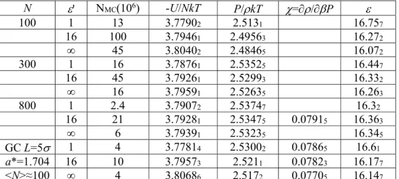
Table 1. Monte Carlo data for the System I (Stockmayer fluid)
N ' NMC(106) -U/NkT P/kT =/P 100 1 13 3.77902 2.5131 16.757 16 100 3.79461 2.49563 16.272 ∞ 45 3.80402 2.48465 16.072 300 1 16 3.78761 2.53525 16.447 16 45 3.79261 2.52993 16.332 ∞ 16 3.79591 2.52635 16.263 800 1 2.4 3.79072 2.53747 16.32 16 21 3.79281 2.53475 0.07915 16.363 ∞ 6 3.79391 2.53235 16.345 GC L=5 1 4 3.77814 2.53002 0.07865 16.61 a*=1.704 16 10 3.79573 2.5211 0.07823 16.177 <N>≈100 ∞ 4 3.80686 2.5172 0.07705 16.147Stockmayer fluid eq. (8), (9): *=0.8, T*=2, *2=1.5. Number of particles N, number of MC
cycles NMC, dielectric constants of the external medium ' and of the dipolar fluid , energy U,
pressure P, compressibility . The last three lines correspond to Grand Canonical simulations with imposed a* activity. For each accumulated average, the end subscript represents one standard deviation on the last digit.
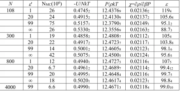
Table 2. Monte Carlo data for the System II (Soft sphere dipolar fluid)
N ' NMC(106) -U/NkT P/kT =/P 108 1 26 0.47452 12.43769 0.021362 1194 20 24 0.49152 12.41309 0.021372 105.68 99 75 0.51571 12.37905 0.021491 95.12 ∞ 26 0.53302 12.35569 0.021632 88.73 300 1 19 0.48582 12.48087 0.021121 1054 20 22 0.49172 12.47237 0.021171 103.88 99 14 0.50012 12.46058 0.021231 98.16 ∞ 42 0.50751 12.45005 0.021241 95.63 800 1 12 0.49401 12.47275 0.021161 1075 20 6.7 0.49612 12.46897 0.021142 99.412 99 20 0.49951 12.46484 0.021161 99.75 ∞ 18 0.50201 12.46174 0.021231 98.84 99 6.6 0.49901 12.46713 0.021184 99.010Figure caption
Figure 1: System I. Dependence on the external dielectric constant '. First three ratio
" ' " '
( ) ( ) ( ) / /
mnl mnl mnl
G r g r g r A N (see eq.(17)) for different couples "/'=1/16 or ∞/16 and different N=100, 300, 800, measured by MC. The curves labelled "GC" correspond to Grand-Canonical simulations with <N>≈100. The horizontal axis expresses r in diameter units. The arrows locate L/2 for the three simulation boxes. Vertical error bars around r=1, 2, 3, 5 represent one standard deviation for each N. The curves labelled DPS and DPS' correspond to the original theoretical prediction (18) 23 and to the extended one (19),
respectively.
Figure 2: System II. Dependence on the external dielectric constant. Same legend as figure 1 with '/"=1/99, 20/99, ∞/99 and N=108, 300, 800. The G110(r) curves have been extended up
to the corner of the boxes, r=L√3/2. Figure 3: System I. Differences gmnl
N(r)-gmnl800(r) between MC data for N=100 (top) and N=300 (bottom). External dielectric constant '=16, close to the bulk value. Statistical error bars are indicated at r=1, 2, 3. These differences should be attributed to the explicit + implicit finite-size corrections.
Figure 4: System II. Differences gmnl
N(r)-gmnl800(r) between MC data for N=108 (top), N=300
(middle) and N=4000 (bottom). External dielectric constant '=99, close to the bulk value. Statistical error bars are indicated at r=1, 2, 3, 4, 5.
Figure 5: System I. Explicit finite-size correction projections expl( )
mnl
E r (divided by N=100 for comparison with grand-canonical simulations). The curves have been derived through (22) from 2nd order pdf derivatives evaluated with finite differentiation of MC data. The symbols
represent the differences between canonical and grand-canonical MC simulations at N=100 and three external dielectric constants e'≡'=16 (full), ∞ (open) and 1 (hatched).
Figure 6: System II. Explicit finite-size correction projections Eexplmnl( )r . Same legend as figure
5.
Figure 7: System I. Symbols: Differences gmnlN-gmnl800-(1/N-1/800)Eexpl.mnl cleaned from the
explicit corrections (22), for N=100 (top) and N=300 (bottom). Statistical error bars shown at
r=1, 2, 3. Curves: Theoretical implicit finite-size corrections derived from the superposition
approximation (23)-(30) (solid lines) or improved with the first correction in (32)-(34). Figure 8: System II. Symbols: Differences gmnlN-gmnl800-(1/N-1/800)Eexpl.mnl cleaned from the
explicit corrections (22), for N=108 (top), N=300 (middle) and N=4000 (bottom). Same legend as figure 7.
Figure 9: Schematic view of the implicit finite-size corrections. The pair correlations between particles 1 and 2 inside the central cell are perturbed by the environment around the periodic image 1' of 1, with the very same orientation, localized at the distance L.
Figure 10: Running Kirkwood factor gK(R) (35) for System II. Symbols: MC brute data for
N=108 and N=4000 with '=99. Lines: MC/MSA results fed with N=108 MC data up to
rmax=2.5 beforehand cleaned without or with different choices for implicit corrections, see
text in Section VI.