Long run economic mobility

HAL Id: tel-01996623

https://tel.archives-ouvertes.fr/tel-01996623

Submitted on 28 Jan 2019

HAL is a multi-disciplinary open access

archive for the deposit and dissemination of sci-entific research documents, whether they are pub-lished or not. The documents may come from teaching and research institutions in France or abroad, or from public or private research centers.

L’archive ouverte pluridisciplinaire HAL, est destinée au dépôt et à la diffusion de documents scientifiques de niveau recherche, publiés ou non, émanant des établissements d’enseignement et de recherche français ou étrangers, des laboratoires publics ou privés.

Long run economic mobility

Ahuitzotl Héctor Moreno Moreno

To cite this version:

Ahuitzotl Héctor Moreno Moreno. Long run economic mobility. Economics and Finance. Université Panthéon-Sorbonne - Paris I, 2018. English. �NNT : 2018PA01E004�. �tel-01996623�

Université Paris 1 - Panthéon Sorbonne - Paris School of Economics

Long run economic mobility

Thèse pour l’obtention du titre de Docteur en Sciences Economiques

Présentée et soutenue publiquement

à Paris, le 19 Février 2018 par :

Ahuitzotl Héctor Moreno Moreno

Jury :

François BOURGUIGNON, Professeur émérite, Paris School of Economics Hippolyte D'ALBIS (Président) Professeur, Université Paris 1

Nora LUSTIG (Rapporteur) Professeure, Tulane University

Thierry MAGNAC (Rapporteur), Professeur, Toulouse School of Economics Christophe MULLER, Professeur, Aix-Marseille School of Economics Elena STANCANELLI (Directrice de thèse) Professeure, Paris School of Economics

« Qui dit étudiant dit parisien ; étudier à Paris, c’est naître à Paris. »

“Les Misérables -Fantine” Victor Hugo (1862)1

Acknowledgements

The idea of movement motivates this work. Hence, I want to dedicate this work to Elsa who has invariably ‘moved’ with me in this roller coaster. To my parents and siblings: their thoughts and prayers travel with me wherever I go.

I want to thank François Bourguignon for having introduced me into this fascinating world of the PhD. In the same line, I want to express my deepest gratitude to Elena Stancanelli who never hesitated in supporting this project without even knowing me. I could have not find a better duet for this venture. You both have lighted a flame on me with kindness and generosity.

Besides my advisors, I would like to thank to my thesis committee: Nora Lustig, Thierry Magnac, Christophe Muller and Hippolyte D'Albis for their encouragement, insightful comments, and hard questions. I am indebted all my teachers (UIA, ITAM, UPF, Sorbonne, ENS, PSE) who have continuously inspired me on this long journey.

Thanks to my peers and friends from Sorbonne University, EHESS, ENS and PSE, for the continuous support and frank friendship (PPD 2012-2013 and PhD 2013-2017): Luis, Bernardo, Macarena, Lourdes, Jaime Montana, Arthur, Emily, Pepe, Oscar, Caro, Remy, Marion, Margarida, Iva, Mattea, Robert@, Pablo, Roy, Jaime, Humberto, Nungh, Cem, Vivianne, Sarah, Benjamin, Simon, Marco, Farshad, Céline, Emanuelle, Can, Woojeong, Alexandra, Marine, Aleky. Undoubtedly, this list is just an unrepresentative sample.

Thanks also to my peers from bureau (223 at the Maison des Sciences Économiques, 218 in PSE). A deep recognition to my colleagues (Olivier, Johana and Vincent) and students in SciencesPo and very importantly to the staff in all these academic institutions: Pauline, Roxane, Weronica, France, Nathalie, Loïc. Thanks to Joerg Luedicke (Senior Statistician, StataCorp LLC).

In one way or another, many people helped me on this project from México. Beatriz Zúñiga, Alejandro Guevara, Fernanda Rodríguez, Patricia Villegas, Roberto Moreno. I also appreciate generous financial support from CONACYT and CEEY. Let me also be grateful to France, and very importantly, to the city of Paris for the generous reception and inspiration over all these years. After all, the great Victor Hugo might be right on this!

I want to thank Eduardo Rodriguez-Oreggia (may he rest in peace), for his academic and moral support, and Rodolfo de la Torre who has sowed on me the academic interest on social inequalities and human development since my early studies. Finally, I want to dedicate all this work to Mexico… with the hope of more peaceful and prosperous moments.

Table of contents

Introduction in English ... 7

From snapshots to a motion picture: On synthetic income panels... 9

Income mobility over a generation: a ‘long run’ motion picture ... 10

Mobility across three generations ... 12

Final remarks ... 15

Résumé Substantiel en Français ... 17

Chapter 1: On synthetic income panels ... 33

1. Introduction ... 35

2. The construction of a synthetic panel ... 37

3. Construction and validation and of a synthetic panel in Mexico: 2002-2005 ... 44

4. The autocorrelation coefficient and the calibration parameters ... 48

5. Estimation results ... 50

6. Concluding remarks ... 56

Appendix 1. Algorithm to calibrate the distribution of the innovation terms ... 57

ANNEX 1... 59

Chapter 2: Three decades of income mobility with

synthetic panels: empirical evidence from Mexico ... 61

1. Introduction ... 63

2. Analytical framework ... 66

3. Trends of income mobility in Mexico ... 72

4. Concluding remarks ... 82

APPENDIX ... 83

Chapter 3: Intergenerational transmission of education

across three generations ... 91

1. Introduction ... 93

2. Data and sample ... 95

3. The general approach to the intergenerational transmission of education. ... 97

4. The effect of grandfather’s education (G0) on their offspring education (G1 and G2) 98 5. The effect of parents’ education on their offspring, G1-G2 ... 103

6. The ‘conditioned’ effect of grandparents’ education on their grandchildren, G0-G2 106

7. Discussion. The direct Vs the extrapolated effect on long run mobility (G02) ... 109

8. Conclusion... 110

ANNEX 1... 112

Final remarks ... 123

Bibliography: ... 125

Introduction in English

Long run economic mobility

The road was rising and falling. A man I saw told

me, “It rises or falls, depending on whether you’re

coming or going. For someone who is going, it

rises; for someone who is coming, it falls.”

Juan Rulfo, “Pedro Páramo”

Economic mobility constitutes a social aspiration in many modern societies.

2

_This

complex notion of prosperity implies that progress is open for everyone regardless of the

fortuitous circumstances of birth or social position. It also evokes the aspiration for

children to be better off than their parents did. A justified concern then emerges when

mobility is determined by individual, intra-generational or inter-generational, origins. Not

only that. This pattern leads to vivid academic and political discussions with direct

implications in terms of public policies. For instance, downward mobility was recently

considered as the defining challenge of our time, by to the former President of the United

States whilst the quest for upward mobility originated the recent creation of The Social

Mobility Commission in the UK.

3

2 _{Social mobility has already paired social inequality recently at least according to Google trends. See}

https://trends.google.com.mx/trends/explore?q=social%20inequality,social%20mobility

Do these reactions correspond to the actual evolution of social mobility? In other words:

1) how can we measure economic mobility with the data available or with the technology

at hand? 2) What are the trends of economic mobility experienced by the current

generation? Moreover 3) how mobile is a society relative to previous generations? These

questions motivate this dissertation. The complexity of these issues may derive in some

sort of paralysis but it is claimed here that it may be possible to learn something about its

evolution by restricting analysis to a couple of key dimensions within the economic

discipline: income and education. This is the scope followed by this research.

The first part of this research addresses the initial of the above-referred interrogations.

The first paper in this dissertation, co-authored with François Bourguignon, is devoted to

deal with the lack of the required data to examine the income dynamics within one

generation. It is well known that longitudinal data is often scarce and is seldom available

in many countries. This is the case even in well-developed countries! This conundrum has

been partially addressed through recent methodological approaches by the so-called

synthetic panels.

The second part of this dissertation is entirely devoted to applied research. More

specifically, the second and third papers describe long run trends of economic mobility in

income and education respectively. The former is devoted to intra-generational mobility

while the later is devoted to inter-generational mobility. Each of them address the second

and third interrogations referred above. In a way this dissertation attempts to improve

the addition of the time dimension in the analysis of economic wellbeing. It attempts to

produce the effect of a motion picture by the use multiple snapshots. The trends contained

herein are far from being perfect and complete but they are based on the use of extensive

data and multiple methods covering three decades and the same number of generations

in each case.

This research expects to expand our knowledge on the empirics of economic mobility as

most of the studies refer to few years of intra-generational mobility or to a couple of

generations only. Furthermore, most of the empirical evidence available refers to Nordic

and highly industrialized countries. Mexico is the canvas of this work but the approaches

and principles followed here could be easily mimicked elsewhere.

Finally, this introduction is not mere to describe technicalities of this work. Instead it aims

at providing a brief and an integrated version of the research with some perspective. The

chapters of this dissertation corresponds actually to self-contained research articles with

detailed methodological descriptions. Readers interested in the technicalities of this

research are therefore referred to the actual chapters or the corresponding papers

following this introduction.

From snapshots to a motion picture: On synthetic income panels

« C’est de la physionomie des années

que se compose la figure des siècles. »

« Les Misérables -Fantine » Victor Hugo (1862)4

The first paper examines the current technology to construct artificial panels and

provides a discussion on its potential uses and implications. The study is motivated by the

fact that longitudinal data, that allows examining the dynamics of individual incomes, are

seldom available in many developing countries. The idea then is to construct synthetic

panel data based on snapshots of the distribution of income that are more and more

accessible under the form of repeated cross-sectional household surveys. A principle that

resembles the one used by the cinematograph to produce the effect of motion.

We examined most of the recent knowledge to construct artificial longitudinal data and

propose a method that uses of multiple methods, i. e. matching techniques, pseudo-panel

estimation and calibration algorithms. To contribute to this branch of the literature we

generalized the original methodology in Dang et al. (2014) and Dang and Lanjouw (2013)

to avoid the most arbitrary assumptions often used. The study also expanded the scope of

analysis by exploring the 'confidence set' of mobility matrices based on key parameters

-in particular the autocorrelation coefficient of first order.

The procedure delivered very satisfactory outcomes and was confirmed by multiple tests

in several potential applications. We learned that the current methodologies are strongly

dependent on their underlying assumptions and, very importantly, the way key

parameters are estimated. In particular the AR(1) coefficient is a key parameter that

requires extremely caution when studying income mobility based on synthetic panel

techniques.

Synthetic panels might still be imperfect machinery. Their notion of motion is still in early

stages of its development and so the empirical evidence emerging from this device is to

be improved. Even the Lumière brothers, who were credited the development of

Cinematograph, were skeptical about their creation in early stages.

5

_{However it is}

unmistakable that their moving images have had a significant influence on modern

societies. Similarly, what it is to be acknowledged here is the emergence of larger, and

better equipped, ‘audience’ interested on the dynamics of income inequality.

Income mobility over a generation: a ‘long run’ motion picture

« Si quelque chose est effroyable, s’il existe une réalité qui

dépasse le rêve, c’est ceci : vivre, voir le soleil,… avoir la

lumière, et tout à coup, le temps d’un cri, en moins d’une

minute, s’effondrer dans un abîme, tomber,… être

là-dessous, et se dire : tout à l’heure j’étais un vivant ! »

« Les Misérables -Cosette » Victor Hugo (1862)6

5 _{"Le cinéma est une invention sans avenir" (The cinema is an invention without any future)” -they}

claimed. See: https://en.wikipedia.org/wiki/Auguste_and_Louis_Lumi%C3%A8re

The above-referred anxiety of social in-mobility (at the beginning of this introduction)

might be well rooted in the fear that changes in the macroeconomic environment

exacerbate this risk of stagnation over the life span. The 2008 global economic crises is a

worldwide recent example. A common concern is that no matter how hard people work,

the floor of individual progress might have been stickier than previously known.

7

_Societal

debates about income mobility are sometimes based on preconceived opinions, political

preferences, limited information or defective methodologies. It appears useful to fill this

gap with empirical evidence using the data and machinery at hand.

Unfortunately, only a handful of countries can challenge these concerns with empirical

evidence from genuine longitudinal surveys. In most cases, these panel surveys cover only

short periods. Other countries simply have to resort to the evidence from artificial data

by the construction of synthetic panels. Studies following this approach, however,

construct a unique panel with data from very distant points in time, which compromises

the panel’s quality and, very importantly, disregard the macroeconomic environment.

Conversely, the vast majority of countries rely on the comparison of two, or multiple,

snapshots based on independent cross-sectional data from household income surveys.

This last approach is not satisfactory as it neglects an essential part of the analysis: the

dynamics of wellbeing.

The second paper of this dissertation then examines the patterns of income mobility over

three decades in Mexico -from 1989 to 2012. The recent economic history of this

developing country allowed examining multiple episodes of the economic cycle. The

analysis focused on the outbreak of two strong economic downturns, one internal in 1995

and the other external in 2008. In both cases the Mexican economy sharply fell by around

7%.

Naturally, the definition and measurement of income mobility is complex, however the

analysis followed three notions of mobility, described in Fields (2010) and Jäntti & Jenkins

(2015), each of which were examined through multiple indicators. These notions are:

positional movement, directional movement and mobility as an equalizer of longer-term

incomes. The strategy then consisted in constructing eleven short-term synthetic panels

using the methodology referred on the previous section.

It is claimed here that the paper contributed to this emerging branch of income mobility

literature by delivering empirical evidence on the long run trends of intra-generational

mobility from a developing country. The paper documents low levels of mobility with

downward mobility during both episodes of economic slump. It follows that that the

mobility patterns experienced during these periods of economic downturn produced an

equalization process.

Mexico emerges as a country characterized by low levels of mobility. This situation

changes in periods of economic crisis where the country is better characterized by an

analogy of glass ceilings with sticky floors. We learn that the patterns obtained by the

construction of synthetic panels are already useful to form societal judgements on the

structure of growth experiences and have already a descriptive value on the distributional

impact of growth.

Mobility across three generations

« La patrie périra si les pères sont foulés

aux pieds. Cela est clair. La société, le

monde roulent sur la paternité. »

« Le père Goriot »

Honoré de Balzac

The idea of mobility also vindicate an inter-generational expectation: children are

expected to attain the fullest stature of what they are capable regardless of their incidental

origins. In other words, children are expected to be better off than their parents and more

distant ancestors. This lead us to the last inquiry stated at the beginning of this

introduction: how mobile is a society relative to previous generations?

The answer to this question required coping with two sensitive issues: 1) having access

to longstanding data that neatly distinguishes parent-children links on a relevant

economic variable-not a simple task, I may say- and, 2) dealing with endogeneity issues.

The first one refers to a problem of data availability and was addressed by the use of a

unique Mexican survey that gathered retrospective information on three generations. The

second lead us to the use of a demanding statistical method: a two fold instrumental

variable approach.

Educated at Lyon’s largest technical high school, La Martiniere, the Lumière brothers

worked for their father, an artist and businessman, who specialised in photographic

equipment. Their story exemplifies the fact that parents not only invest monetary

(financial) and non-monetary (time) resources on their offspring but also transmit part

of their unobserved ability to their children. This transfer is likely to produce biased

estimates of intergenerational mobility using OLS - the most widely statistical technique

used in a large body of this branch of the literature.

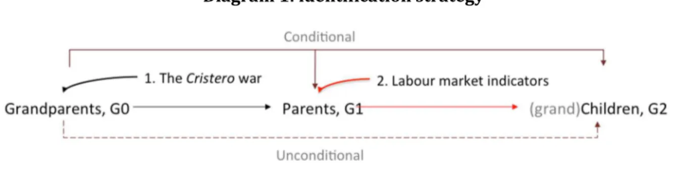
The endogeneity of paternal schooling was addressed by the use of a two-fold

instrumental variable approach described in Diagram 1. A natural experimental set up

from a regional war that occurred at the beginning of the 20th century was exploited to

instrument years of schooling of the “grand-father” generation whereas labour market

indicators, a well-known instrument in the labour economics literature, served as an

instrument for the education of the “parents” generation.

8

_{This unified framework}

allowed examining the intergenerational transmission of human capital across three

generations and, very importantly allowed comparing the conditional and the

unconditional effect of grand-parental education on their grandchildren. The following

diagram illustrates this approach.

8 _{La Cristiada was a massive armed conflict that lasted three years from 1926-1929. This religious conflict}

can be briefly summarized by a massive rural rebellion in the western and central states of Mexico after the enforcement of anticlerical laws that emerged from the Mexican Constitution of 1917.

Diagram 1: identification strategy

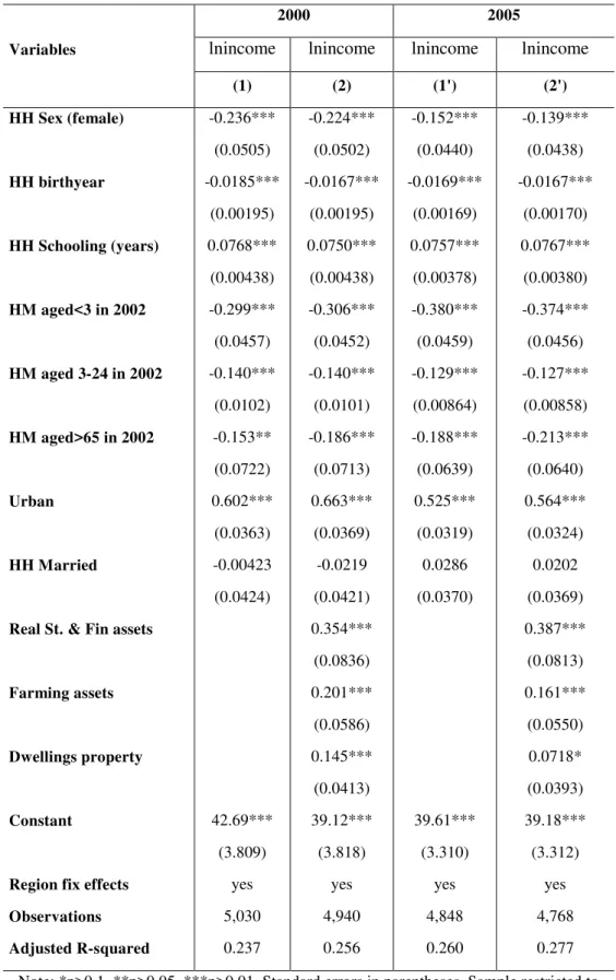
The paper shows that parental education has a significant effect on their children’s

education. It also shows that the IV estimate is larger than the OLS estimate, which implies

that accounting for endogeneity unveils a larger importance of familiar background (less

educational mobility than traditionally considered) than ignoring it. This holds true for

both the grandparent-parent link as well as for the parent-child link.

We learned that parental education is the most important family background in the

children’s years of education though it seems to play a lesser role in successive

generations (implying more mobility with every new pair of generations). Very

importantly, we also learned that beyond the findings of two contiguous generations,

results also suggest that the influence of the grandparents’ educative legacy, conditional

on parental education, did not seem to reach the second generation -in Mexico. The origins

of inequality are long rooted but they could be tackled from one generation to the

following one.

Final remarks

The roads of our lives are constantly moving: rising and falling –as the initial epigraph

implied. In a democratic context, it is useful to know, whether our society provides the

chance to get ahead regardless of our origins, or whether this chance is ruled or doomed

by them.

If good fortune is only determined to a group that is constantly “going and rising” whereas

the lack of upward mobility is predetermined to those who are systematically “coming

and falling” by their individual backgrounds, then it may well be the case that we may

actually be facing a defining challenge of our time -like recently stated in the USA. We may

also want to know, from a policy perspective, whether the long run mobility trends

justifies the creation of a Social Mobility Commission or other public policies -like the one

created in the UK.

Empirical evidence is needed to foster these deliberations -which are often absent in

many modern societies. This dissertation may well be an invitation to sustain this kind

conversation.

Résumé Substantiel en Français

La mobilité économique à long terme

« Le chemin allait par monts et par vaux.

Il monte ou descend selon que l’on va ou que l’on vient.

Pour qui va, il monte ; pour qui vient, il descend. »

Juan Rulfo,

« Pedro Páramo »

La mobilité économique est une des aspirations de toute société moderne. Cette

notion assez complexe de la prospérité implique que le progrès économique est

une possibilité pour chacun, peu importe les circonstances fortuites de sa

naissance ou de sa position sociale. Cette notion évoque également l’aspiration de

la part des enfants, de s’en sortir mieux que leurs parents. Ces suppositions qui

sembleraient des évidences soulèvent pourtant une préoccupation, tout-à-fait

justifiée, où moment où la mobilité se voit déterminée par les origines de chaque

personne, soient celles individuelles ou familiales.

Ce le sujet de la mobilité amène ainsi à des discussions politiques ou universitaires

qui ont un impact direct sur les politiques publiques. Par exemple, la mobilité vers

le bas a été récemment considérée « le défi définissant de notre temps » par l’ancien

président des États-Unis, tandis que la quête de la mobilité vers le haut a été l’idée

à l’origine de la création de la Commission pour la mobilité sociale au Royaume Uni.

Comment peut-on savoir si ces réactions politiques correspondent à la véritable

évolution de la mobilité sociale ? C’est-à-dire : 1) peut-on mesurer la mobilité

sociale avec les données ou la technologie disponibles aujourd’hui ? 2) Quelles sont

les tendances de la mobilité sociale qui a traversées la génération actuelle ? Ou

encore 3) à quel point la société actuelle est-elle mobile par rapport aux anciennes

générations ?

Ce sont les trois questions à la base de cette thèse. Certes, la complexité de ces

problématiques pourrait nous amener vers une sorte de paralyse, mais nous

soutenons ici que c’est possible de connaître encore plus sur l’évolution de la

mobilité sociale en restreignant son analyse à quelques dimensions dans le champ

de l’économie : le revenu et l’éducation. Ce parcours est donc l’objectif de notre

recherche.

La première grande partie de la thèse, composée par le premier des trois articles,

s’occupe de la première des questions posées plus haut. Co-écrit avec François

Bourguignon, cet article s’attaque au problème du manque des données

nécessaires pour l’analyse des dynamiques du revenu à l’intérieur d’une

génération. Il est avéré que les données longitudinales sont rares et très peu

disponibles dans la plupart des pays, ce qui est vrai même pour les pays développés

! Nous avons essayé d’assembler ce casse-tête par des approches méthodologiques

récentes, telles que les « panels synthétiques », une méthodologie normalement

utilisée pour l’analyse des dynamiques de la pauvreté.

La seconde grande partie de la thèse est dédiée à la recherche appliquée. Les

articles deux et trois décrivent, plus spécifiquement, les tendances à long terme de

la mobilité économique pour le revenu et pour l’éducation, respectivement. Le

deuxième papier s’occupe de la mobilité intra-générationnelle, tandis que le

troisième est dédié à la mobilité intergénérationnelle. Tous les deux répondent aux

questions deux et trois posées plus en haut, en cherchant d’améliorer la façon dont

la dimension temporaire este incluse dans l’analyse du bien-être économique, ceci

avec pour but de reproduire l’effet d’un film fait avec plusieurs clichés. Bien que les

tendances présentées ici soient loin d’être parfaites ou même complètes, elles se

basent dans l’utilisation de larges quantités de données et de différentes méthodes

pour contenir trois décades et trois générations dans chaque cas.

Cette thèse cherche à élargir le savoir expérimental sur la mobilité économique, vu

que la plupart des études ne prennent en compte que quelques années de mobilité

intra-générationnelle ou à peine quelque génération. En outre, la plupart des

résultats des expériences existantes font référence aux pays scandinaves ou à des

pays fortement industrialisés. Pour cette thèse nous avons donc pris l’exemple du

Mexique, mais les approches et les principes méthodologiques utilisés pourront

être appliqués à n’importe quel autre pays.

Enfin, ce n’est pas le but de cette introduction de décrire les aspects techniques du

travail présenté. L’objectif est plutôt de faire une mise en perspective à travers une

explication succincte. Chaque chapitre de la thèse est un article indépendant avec

des descriptions méthodologiques détaillées. Les lecteurs intéressés aux aspects

techniques pourront donc s’adresser directement à chaque chapitre.

1. De la succession de clichés au film en mouvement : les panels

synthétiques du revenu

« C’est de la physionomie des années

que se compose la figure des siècles. »

« Les Misérables -Fantine » Victor Hugo (1862)9

Le premier article étudie les techniques actuelles pour la construction de panels

artificiels, en apportant des éléments pour mieux comprendre leur utilisation et

leurs implications. Cette analyse est motivée par le fait que les données

longitudinales qui normalement permettent l’étude de la dynamique du revenu

individuel sont rares dans les pays en développement. L’idée est donc de construire

des données de panel synthétiques basées sur des « clichés » de la distribution du

revenu, qui sont en revanche de plus en plus disponibles grâce à l’accessibilité des

enquêtes de coupe transversale sur le revenu du ménage. Ce principe ressemble

celui utilisé par le cinématographe pour la reproduction de l’effet de mouvement.

On a analysé ici la plupart de la littérature scientifique sur la construction de

données longitudinales artificielles par différentes méthodes, y compris les

techniques de matching, les estimations par pseudo-panel et la calibration

d’algorithmes. Dans le but de contribuer à cette branche des études économiques,

nous avons généralisé la méthodologie originale trouvée en Dang et al. (2014) et

en Dang and Lanjouw (2013) pour éviter leurs suppositions les plus arbitraires.

Notre approche a été aussi d’élargir la portée de l’analyse en explorant la ‘région

de confiance’ des matrices de mobilité basées dans des paramètres clés,

notamment dans le coefficient d’autocorrélation de première ordre.

Vérifiée à partir de plusieurs tests pour de différentes applications potentielles,

cette procédure a donné des résultats satisfaisants. L’exercice nous a permis

d’observer la façon dont les paramètres clé sont estimés –les AR(1), ainsi que

d’apprendre que les méthodologies actuelles dépendent fortement de leurs

suppositions sous-jacentes. Nous conseillons donc d’agir avec précaution au

moment d’utiliser cette technique pour examiner la mobilité du revenu.

Le présent article améliore la méthodologie d'étalonnage de ces panneaux

synthétiques dans plusieurs directions. Nous exploitons la dimension transversale

d'une enquête par panel mexicaine représentative au niveau national pour évaluer

la validité de cette approche. La matrice de mobilité du revenu dans le panel

synthétique sur deux régimes utilisées se révèle être très proche de la matrice

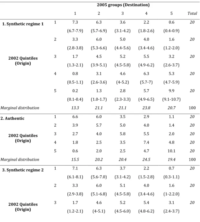
observée dans l’authentique panel (voir table 1). Le chapitre comprend un résumé

pratique menant à la construction d'un panel synthétique pour faciliter sa mise en

œuvre par les praticiens intéressés.

C’est fort possible que la méthodologie des panels synthétiques soit encore

imparfaite. Même les frères Lumière, connus pour l’invention du cinématographe,

étaient sceptiques de leur propre création , mais leurs images motrices ont eu sans

doute une influence significative dans les sociétés modernes : ce qu’il faut retenir

au-delà de la machine, est l’émergence d’un public avide. Similairement,

l’importance de la construction des panels synthétiques peut être mesurée en

fonction de la demande d’analyses longitudinales du bienêtre humain.

Table 1. Matrice de mobilité du revenu, 2002-2005.

- Porcentaje -

2005 groups (Destination) 1 2 3 4 5 Total Régime 1 2002 Quintiles (Origine) 1 7.3 6.3 3.6 2.2 0.6 20 (6.7-7.9) (5.7-6.9)* (3.1-4.2)* (1.8-2.6) (0.4-0.9) 2 3.3 6.0 5.0 4.0 1.6 20 (2.8-3.8) (5.3-6.6)* (4.4-5.6)* (3.4-4.6)* (1.2-2)* 3 1.7 4.5 5.2 5.5 3.2 20 (1.3-2.1) (3.9-5.1)* (4.5-5.8)* (4.9-6.2)* (2.6-3.7) 4 0.8 3.1 4.6 6.3 5.3 20 (0.5-1.1) (2.6-3.6) (4-5.2) (5.7-7) (4.7-5.9)* 5 0.2 1.3 2.8 5.7 9.9 20 (0.1-0.4) (1-1.7) (2.3-3.3)* (4.9-6.5) (9.1-10.7)* Authentique 2002 Quintiles (Origine) 1 6.6 6.0 3.5 2.9 1.1 20 2 3.9 5.7 5.0 4.0 1.4 20 3 2.7 4.0 5.8 5.5 2.0 20 4 1.8 2.5 3.5 7.4 4.8 20 5 0.6 2.0 2.5 4.7 10.1 20 Régime 2 2002 Quintiles (Origine) 1 7.1 6.3 3.7 2.2 0.7 20 (6.1-8.1)* (5.6-7)* (3.1-4.2)* (1.5-2.8) (0.3-1.1)* 2 3.3 6.0 5.1 4.0 1.6 20 (2.9-3.8) (5.1-6.8)* (4.5-5.8)* (3.4-4.6)* (1-2.2)* 3 1.7 4.6 5.2 5.4 3.1 20 (1.2-2.1) (4-5.1) (4.5-6)* (4.8-6.2)* (2.4-3.7) 4 0.8 3.1 4.7 6.4 5.1 20 (0.4-1.2) (2.5-3.7) (4.1-5.3) (5.5-7.3) (4.4-5.8)* 5 0.3 1.4 2.8 5.7 9.8 20 (0.1-0.5) (0.9-1.9) (2.2-3.4)* (5-6.4) (8.7-10.8)* Notes: 95% C.I. in parenthèses. Voir table 3, chapitre 1.

2. Mobilité économique tout au long d’une génération : un film ‘à long terme’

« Si quelque chose est effroyable, s’il existe une réalité qui

dépasse le rêve, c’est ceci : vivre, voir le soleil,… avoir la

lumière, et tout à coup, le temps d’un cri, en moins d’une

minute, s’effondrer dans un abîme, tomber,… être

là-dessous, et se dire : tout à l’heure j’étais un vivant ! »

« Les Misérables -Cosette » Victor Hugo (1862)10

La crainte de l’immobilité sociale dont on parlait plus en haut, pourrait très bien

avoir ses racines dans la peur que les fluctuations dans le climat

macro-économique puissent aggraver le risque de stagnation tout au long de la vie des

individus. Les crises économiques globales de 2008 n’en sont qu’un exemple récent

de ceci. En effet, une préoccupation fréquente est le fait que malgré le travail dur

des gens, les planchers du progrès individuel s’avèrent en fait plus gluants de ce

qu’on pensait . En tout cas, les débats sur la mobilité du revenu sont très souvent

basés sur des idées reçues, des références politiques ainsi que sur des

méthodologies défectives ou de l’information limitée. Il semble donc utile de

remplir ce besoin avec des résultats empiriques en se servant des données et des

techniques à notre portée.

Malheureusement à peine quelques pays peuvent utiliser des données provenant

d’enquêtes longitudinales pour prendre en charge ces préoccupations, tandis que

d’autres nations se résolvent avec des données artificielles crées avec des panels

synthétiques. En construisant très souvent un panel unique avec des données

provenant des points éloignés dans le temps, ces études tendent à compromettre

leur qualité et ne prennent pas en considération l’environnement

macroéconomique.

Mais la vaste majorité des pays de la planète s’appui sur la comparaison de deux

ou plusieurs ‘clichés’ (snapshots) provenant des coupes transversales

indépendantes de données d’enquêtes du revenu des ménages. Cette approche est

loin d’être satisfaisant, car elle néglige une partie essentielle de l’analyse : les

dynamiques du bienêtre.

Le deuxième article composant cette thèse étudie les patrons de la mobilité du

revenue au Mexique tout au long de trois décennies –de 1989 à 2012. L’histoire

économique récente de ce pays en développement nous a permis d’examiner

différents épisodes du cycle économique (voir graphique 1). Notre analyse se

concentre ainsi dans l’explosion de deux baisses économiques, une interne en 1995

et l’autre externe en 2008. Dans les deux cas, l’économie mexicaine a subi une

baisse d’environ 7%.

Bien que la définition et la mesure de la mobilité du revenu soient complexes, notre

analyse est basée sur trois notions de mobilité, telles qu’elles ont été établies par

Fields (2010) et par Jäntii & Jenkins (2015) en faisant des examens à partir de

différents indicateurs. Il s’agit des notions suivantes : mouvement positionnel,

mouvement directionnel et mobilité en tant qu’équaliseur de revenus de long

terme. La stratégie a donc consisté en la construction d’onze panels synthétiques à

court terme réalisés avec la méthodologie décrite dans la section précédente.

Graphique 1

Nous soutenons que cet article contribue à cette branche émergeante de la

littérature sur le revenu économique dans la mesure où il rend des résultats

empiriques sur les tendances de la mobilité intra-générationnelle à long terme

dans un pays en développement. L’article rend compte des bas niveaux de mobilité

et de la mobilité vers le bas pendant les deux périodes de récession économique.

On peut conclure ainsi que les patrons de mobilité économique observés pendant

ces périodes produisent un processus d’égalisation.

Le Mexique se dessine ainsi comme un pays avec des bas niveaux de mobilité. Cette

situation bouge dans des périodes de crise économique, où le pays est bien

représenté par l’analogie des planchers gluants et les plafonds de verre (voir

graphique 2). Ceci nous permet d’observer que les patrons sortis de la construction

des panels synthétiques sont utiles pour informer les opinions sur la structure de

la croissance et pour l’obtention de valeurs descriptives sur son impact distributif.

2009 1995 -6 -4 -2 0 2 4 6 8 10 Pe rce nt 1980 19821984198619881990199219941996199820002002200420062008201020122014 Year

Source: IMF Gross domestic product, constant prices (National currency). Mexico, 1980-2014

Graphique 2

-. 4 -. 35 -. 3 -. 25 -. 2 -. 15 -. 1 -. 05 0 .0 5 .1 .1 5 .2 D 1 in de x 8992 9294 9496 9698 9800 0002 0204 0406 0608 0810 1012 Periods

Note: 95% Conf. Int in shaded area

3. Mobilité éducative à travers trois générations

« La patrie périra si les pères sont foulés

aux pieds. Cela est clair. La société, le

monde roulent sur la paternité. »

« Le père Goriot »

Honoré de Balzac

L’idée de la mobilité revendique une expectative intergénérationnelle positive : les

enfants sont censés atteindre le maximum de leur capacités malgré l’incertitude de

leurs origines. C’est-à-dire, ils sont censés s’en sortir mieux que leurs parents et

leurs ancêtres lointains. Ce principe nous amène a la dernière des questions posées

au début de cette introduction : à quel point une société est-elle mobile par rapport

aux générations précédentes ?

La réponse à cette interrogation a voulu l’attention à deux problèmes : 1) l’accès à

des données de longue date qui permettent l’observation des liens entre parents et

enfants sur une variable économique importante –ce qui n’est pas évident- et 2) le

traitement des problèmes d’endogéneité. Le premier point répond au problème de

la disponibilité des données auquel on s’attaqué avec l’utilisation d’une enquête

mexicaine recueillant de l’information rétrospective de trois générations. Pour le

second nous avons dû utiliser une méthode statistique : l’approche de la variable

instrumentale.

Éduqués à la Martinière, le plus grand lycée de Lyon, les frères Lumière ont

travaillé pour leur père, artiste et homme d’affaires spécialisé en équipe

photographique. Leur histoire donne un exemple du fait que les parents ne font pas

uniquement un investissement financière ou temporaire dans leurs enfants, mais

ils leur transfèrent aussi leur habilité inobservée. Ce transfert tend à produire des

estimations biaisées de la mobilité intergénérationnelle avec l’utilisation d’OLS –la

technique statistique la plus utilisée dans la plupart de la littérature de ce domaine.

L’endogéneité de la scolarité des parents a été adressée par l’utilisation d’une

variable instrumentale double, telle qu’elle est décrite dans la figure nº1. Une

expérience naturelle à partir d’une guerre régionale ayant lieu au début du XXe

siècle (voir carte 1) a été utilisée pour instrumenter les années de scolarité de la

génération des « grands-parents » tandis que les indicateurs du marché du travail,

un instrument assez connu dans la littérature de l’économie du travail, ont été

utilisés pour instrumenter l’éducation de la génération des « parents

». Cet encadrement unifié nous a permis d’analyser la transmission

intergénérationnel du capital humain à travers trois générations, et notamment de

comparer les effets conditionnel et non-conditionnel de l’éducation des

grands-parents envers celle de leurs petits enfants. Une fois équipé d'un ensemble de

stratégies d'identification pour chacune des deux premières générations, l'article

examine la transmission intergénérationnelle du capital humain sur trois

générations.

Plus spécifiquement, le papier étudie l'effet de l'éducation grand-parentale sur

l'éducation de leurs petits-enfants, conditionnel à l'éducation des parents dans le

cadre d'une approche variable instrumentale. L'analyse montre d'abord que

l'éducation parentale est le milieu familial le plus important dans les années

d'éducation des enfants, bien qu'elle semble jouer un rôle moindre dans les

générations successives.

Diagramme 1: stratégie d'identification

L’article permet aussi d’observer que l’éducation des parents a un effet significatif

sur l’éducation de leurs enfants. Il montre également que l’estimation IV est plus

grande que l’estimation OLS, ce qui implique que le fait de prendre en compte

l’endogéneité dévoile une importance majeur du milieu familial (moins de mobilité

éducative de ce qui était traditionnellement considéré). Ceci est vrai soit pour le

lien entre les grands-parents et les parents que pour celui d’entre les parents et les

enfants (voir table 2).

Mobilité éducative à travers trois générations, Mexico

Dep. Var.: Education petits-enfants

Indep. Var / Method: OLS IV 1

Reduced form

Education parentale 0.353*** 0.418***

-0.0369 -0.0512

Education grand-parentale 0.0239 -0.015

-0.0357 -0.159

Sex, G2, G1 Yes Yes

Birthyear, G1, G2 Yes Yes

Wealth, G0, G1 Yes Yes

Number of children, G0, G1 Yes Yes

State fixed eff. Yes Yes

Note: Voir Table 5. Chapitre III

Nous avons ainsi découvert que l’éducation parentale est le trait le plus important

pendant les années d’éducation des enfants, mais pas autant dans les générations

successives (ce qui implique plus de mobilité toutes les deux générations). Si

l’héritage éducatif des grands-parents est conditionnel de l’éducation parentale, les

résultats permettent aussi de d’observer qu’il ne l’est plus pour la seconde

génération.

Remarques finales

Les chemins de nos vies sont dans un mouvement perpétuel : par monts et par

vaux comme dans l’épigraphe au début de cette introduction. Dans une société

démocratique, il semble utile de savoir si notre appartenance sociale nous permet

de nous en sortir malgré nos origines, ou si au contraire, notre destin est voué à

l’échec à cause d’elles.

Si la bonne chance est prérogative d’un seul groupe qui peut constamment «

monter et s’élever » tandis que le manque de mobilité vers le haut appartient

uniquement à ceux qui sont systématiquement en train de tomber à cause de leur

entourage familier ou leur histoire individuelle, alors on se trouve bien devant « le

défi définissant de notre temps » comme il a été déclaré aux États-Unis. Nous

pourrions également essayer de comprendre comment, à partir d’une perspective

de politiques publiques, les tendances de mobilité à long terme justifient la création

d’une commission pour la mobilité sociale ou d’autres politiques publiques comme

celle crée au Royaume Uni. Il nous faut en effet, des résultats empiriques pour

répondre à ces délibérations, très souvent absentes des sociétés modernes. Cette

thèse est peut-être une invitation osée à mettre en marche cette conversation.

Chapter 1:

On synthetic income panels

11

« C’est de la physionomie des années

que se compose la figure des siècles. »

« Les Misérables » Victor Hugo (1862)12

11 _{Based on a co-authored paper with François Bourguignon.} 12_{Tome I – Fantine , Chapitre II : Double quatuor »}

Abstract

13

In many developing countries, the increasing public interest for economic inequality and

mobility runs into the scarce availability of longitudinal data. Synthetic panels based on

matching individuals with the same time-invariant characteristics in consecutive

cross-sections have been proposed as a substitute to such data - see Dang and Lanjouw (2014).

The present paper improves on the calibration methodology of such synthetic panels in

several directions: a) it abstracts from (log) normality assumptions; b) it improves on the

estimation of auto-correlation of unobserved determinants of (log) earnings; c) it

considers the whole mobility matrix rather than mobility in and out of poverty. We exploit

the cross-sectional dimension of a national-representative Mexican panel survey to

evaluate the validity of this approach. The income mobility matrix in the synthetic panel

calibrated on the former turns out to be very close to the observed matrix in the latter.

The chapter includes a practical summary leading to the construction of a synthetic panel

to facilitate its implementation by interested practitioners.

13_{We gratefully acknowledge comments on previous versions from Andrew Clark (PSE-LSE), Hai Ann Dang}

(World Bank), Rodolfo de la Torre (CEEY), Dean Jolliffe (World Bank), Marc Gurgand (PSE), Thierry Magnac (TSE), Jaime Montaña (PSE), Christophe Muller (AMSE), Umar Serajuddin (World Bank), Elena Stancanelli (PSE- CNRS) and attendants to internal seminars at the Paris School of Economics (WIP and SIMA) and NEUDC 2015 at Brown University (USA).

1. Introduction

The issue of income mobility is inextricably linked to the measurement of inequality and poverty. Incomes of persons A and B may be very different at both times _{� and �′. But can this difference be} truly considered as inequality if persons A and B switch income level between _{� and �′? Likewise,} should a person above the poverty line in period 1 be considered as non-poor if it is below the line in period 2? Clearly, this depends on how much above the line she was in the first period and how much below in the second. Measuring inequality and poverty in a society may thus be misleading if one uses only a snapshot of income disparities at a point of time instead of individual income sequences.

Longitudinal or panel data that would permit analysing the dynamics of individual incomes are seldom available in developing countries. Yet, snapshots of the distribution of income are increasingly available under the form of repeated cross-sectional household surveys. The idea thus came out to construct synthetic panel data based on these data by appropriately matching individuals in the two cross-sections with the same time invariant characteristics but with the appropriate age difference in two consecutive cross-sections. Such synthetic panels potentially offer advantages over real ones. They may cover a larger number of periods and they suffer much less from typical panel data problems like attrition, non-response and measurement errors (Verbeek, 2007). But, of course, their reliability depends on the quality of the matching method.

This type of approach has received much attention recently (Dang et.al. , 2014; Cruces et al., 2011, Ferreira et al., 2011,). These papers are based on the methodology designed in Dang et al. (2014) - which was circulated as a working paper in 2011.14 This methodology permits to obtain an upper and a lower bound of mobility, in and out of poverty, by matching individuals with identical time invariant characteristics and assuming that that part of their (log) income that is independent of these characteristics is normally distributed across the two periods with a correlation coefficient equal respectively to 0 or 1. In an unpublished paper, Dang and Lanjouw (2013) refined this method by providing a point estimate of income mobility based on a correlation coefficient estimated through pseudo-panel techniques applied to the two cross-sections.

Unsurprisingly, the properties of such synthetic panels are strongly dependent on the assumptions being made and the way key parameters are estimated. In the methodology designed by Dang and Lanjouw (op. cit.), for instance, the bi-normality assumption made on the joint distribution of initial and final incomes – conditionally on time invariant characteristics - and the way the associated coefficient of correlation is estimated strongly influence the synthetic income mobility matrix. As this coefficient is bound to have a strong impact on the extent of estimated mobility, the estimation method and its precision clearly are of first importance.

The purpose of the present paper is to analyze in some depth the properties of synthetic panels and their precision in reproducing income dynamics. This is done first by generalizing the original estimation and simulation methodology in Dang et al. (2014) and Dang and Lanjouw (2013) so as to avoid the most arbitrary assumptions found there and then by exploring the 'confidence set' of mobility matrices generated by the confidence intervals on key parameters as the correlation coefficient mentioned above.

Departure from previous work includes explicitly involving the calibration of synthetic panels within the realm of AR(1) processes, conditional on time invariant, a more robust estimation of the associated auto-regressive coefficient, and going beyond the normality assumption. Also, the focus of the exercise is the whole income mobility matrix, rather than the share of population moving in and out of poverty.

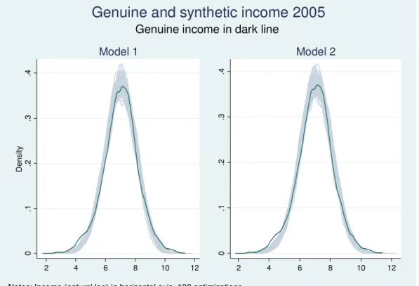
The validity and the precision of the synthetic panels constructed with that method are tested by comparing the synthetic mobility matrix obtained on the basis of the initial and terminal cross-sections of a Mexican panel household survey between 2002 and 2005 and the observed actual matrix in that survey. Although no formal test is possible on a single observation, the results are encouraging as the synthetic joint distribution of initial and final incomes is rather close to the joint distribution in the authentic panel. However, simulations performed by allowing the AR(1) coefficient to vary within its estimation confidence interval show a rather high variability of the synthetic mobility matrix and associated income mobility measures. This should plead in favour of extreme caution in analyzing income mobility based on synthetic panel techniques.

There is also a connection with the growing literature of partial identification literature.15 _This

paper addresses a problem similar to the “classic” ecological inference (EI) problem where individual-level and aggregate data are combined to predict an individual-level outcome of interest (the outcomes of interests are observed only at aggregated level, while the conditional covariates are observed at the individual level). However, EI literature explicitly frames this lack

of longitudinal data in the program evaluation framework - the problem then becomes one of identifying the mean counterfactual outcome in a treatment effect model (Cross & Maski, 2002). Another association with this literature arises by the aim of obtaining bounds on these counterfactual outcomes. Fan, Sherman & Shum (2016) for instance obtained these bounds as functionals of quintile functions of generated variables. In our approach, these bounds are generated by the confidence set of an autoregressive parameter of first order. A closer connection with this literature is still to be made but it is reassuring that the copula literature, like in Fan, Sherman & Shum (2016) and Foster and Rothbaum (2015), would be an avenue of future research.

The paper is structured as follows. Section two and three describe methodology used in this paper to construct synthetic panels based on AR(1) conditional income processes, comparing it to previous work in this area. Section four present the data used to test this methodology. Section five presents the central results of the whole procedure and compare the central estimate of the synthetic income mobility matrix and various mobility measures to those obtained from the authentic panel. In section six, some sensitivity analysis is performed on various aspects of the methodology so as to test its robustness. The last section concludes.

2. The construction of a synthetic panel

2.1 Matching techniques and the synthetic panel approach

Consider two rounds of independent cross-section data at time t and t'. If _{��(�)��} denotes the (log) income in period _{�′ of an individual � observed in period �} 16, what is actually observed is _{��(�)�}

and ��(��)��. Constructing a synthetic panel is somehow 'inventing' a plausible value for ��(�)�� .

A first step is to account for the way in which time invariant individual attributes, z, may be remunerated in a different way in periods _{� and �′. To do so, an income model defined exclusively} on time invariant attributes observed in the two cross-sections is estimated with OLS:

��(�)�= ��(�)��+ ��(�)� � = �, �′ (1)

where _�� represents the vector of ‘returns’ to fixed individual attributes, z, and _��(�) denotes a ‘residual’ that stands for the effect of time variant individual characteristics and other unobserved time invariant attributes. Fixed attributes may include year of birth, region of birth, education, parent’s education, etc. More on this in a subsequent section. For now it is just enough to stress

that it would not make sense to introduce time-varying characteristics in the income model (1), even though some of them may be observed as their value in the terminal (or initial) year are essentially unknown.

Denote _��� and _{�̂�(�)�} and _���� at time _{� = �, �′ respectively the vector of estimated returns, the} corresponding residuals and their variance as obtained from OLS:

��(�)� = ��(�)���+ �̂�(�)� � = �, �′ (2)

Consider now an individual _{� observed in the first period, �. Part of the dynamics of her income} between _{� and �′ stems from the change in the returns of fixed attributes, or ��(�)����}�− ��_�� and

can be inferred from OLS estimates. The remaining is the change in the residual term: �̂�(�)��−

�̂�(�)�. The problem is that the first term in this difference is not observed. The issue in constructing

a synthetic panel thus is the way of finding a plausible value for it. Let _{�̃�(�)��} be that 'virtual' residual. At this stage, the only information available about it is that it has zero mean and variance ����� across the whole population.

2.2 Previous approaches

In their first attempt at constructing synthetic panels, Dang et al. (2011, 2014) simply assumes the virtual residual at time t' to be normally distributed conditional on the residual �̂�(�)�at time t

with an arbitrary correlation coefficient, _{�. Assuming that the initial residual is also normally} distributed, then the synthetic income mobility process can be described by the joint cdf:

Pr���(�)�≤ #; ��(�)�� ≤ #�� = % &# − ��(�)���

��� ,

#�_{− �}

�(�)����

���� ; �'

where N( ) is the cumulative probability function of a bi-normal distribution with correlation coefficient �.

In their initial paper, Dang et al. (2011,2014) considered the two extreme cases of � = 0 and � = 1, so as to obtain an upper and a lower limit on mobility. Applying this approach to the probability of getting in or out of poverty in Peru and in Chile, the corresponding ranges proved to be rather broad. In other words, the change _�����− ��_�� in the returns to fixed attributes was playing a limited

role in explaining income mobility.

In a later, unpublished paper, Dang & Lanjouw (2013) generalized the preceding approach by considering a point estimate rather than a range for the correlation between the initial and

terminal residuals. Their method consists of approximating the correlation between the (log) individual incomes in the two periods t and t', �*, by the correlation between the mean incomes of birth cohorts in the two samples,�*+_{, as in pseudo-panel analysis. Then, the covariance between}

(log) incomes is approximated by _,-.*= �*+. �_* /

�_�*

/�

� _{where �*}

0

� _{is the variance of (log) income at}

time _{�. Then it comes from the two equations in (2), if both applied to the same sample of} individuals, that:

,-.*= ���123(�)���+ ,-.₄ (3)

where _{123(�) is the variance-covariance matrix of the fixed characteristics, z, and ,-.4} the covariance between the residual terms. With an approximation of_,-.* , and estimates of _�� and _���, as well as of the variance of the residual terms, it is then possible to get an approximation of the correlation coefficient between these residuals.

This appears as a handy way of getting an estimate of the correlation coefficients between initial and terminal cross-sections by relying on their pseudo-panel dimension. Yet, it will be seen below that this method is not fully correct.

2.3. Synthetic panels with AR(1) residuals

The methodology proposed in this paper assumes explicitly that the residual in the income model (2) for a given individual_{�(�) follows an first order auto-regressive process, AR(1), between the} initial and the final period. If it were observed at the two time periods _{� and �′ the income of an} individual would thus obey the following dynamics:

��(�)�� = �_�(�)�_��+ �_�(�)�� 5��ℎ �_�(�)�� = ��_�(�)�+ 7_�(�)�� (4)

where the ‘innovation terms’, _7�(�)�, are assumed to be orthogonal to _{��(�)�}and i.i.d. with zero mean and variance _�8�.

The autoregressive nature of the residual of the basic income model can be justified in different ways. The time varying income determinants may be AR(1), the returns to the unobserved time invariant characteristics may themselves follow an autoregressive process of first order or, finally, stochastic income shocks may be characterized by this kind of linear decay. It is reasonably assumed that the auto-regressive coefficient, _{�, is such that: 0 < � < 1.}

Consider now the construction of the synthetic panel when the parameters of the AR(1) model in equation (4) are all known. The issue of how to estimate these parameters will be tackled in the

next section. As described in the previous section, income is regressed on time invariant attributes in the two periods as in (2). Equation (4) can then be used to figure out what the residual of the income model, _{�̃�(�)��}, could be in time _{�′ for observation �(�):}

�̃�(�)�� = ��̂�(�)�+ 7:�(�)��

where7:_{�(�)��}has to be drawn randomly within the distribution of the innovation term, of which cdf will de denoted _;��8. If estimations or approximations of _{� and the distribution ;��}8 are available, the virtual income of individual i(t) in period _{�′ can be simulated as:}

�:�(�)�� = ��(�)����+ ��̂�(�)�+ ;��8<=(>�(�)) (5)

where >_�(�) are independent draws within a (0,1) uniform distribution. After replacing _{�̂�(�)�} by its expression in (2), this is equivalent to:

�:�(�)�� = ��_�(�)�+ �_�(�)���_��− ���_�� + ;_�8 <=� �>_�(�)� (6)

Thus the virtual income in period t' of individual i(t) observed in period t depends on his/her observed income in period t, ��(�)�, his/her observed fixed attributes, ��(�), and a random term

drawn in the distribution _;��8. Because those virtual incomes are drawn randomly for each individual observed in period t, the income mobility measures derived from this exercises necessarily depends on the set of drawings. Various simulations will have to be performed to compute the expected value of these measures - and, actually, their distribution.

The two unknowns, _{� and ;�}?�( ) must be approximated or 'calibrated' in such a way that the

distribution of the virtual period _{�′ income, �:�(�)��}, coincides with the distribution of _{��(��)��} observed in the period t' cross-section. We first focus on the estimation of the auto-regressive coefficient, _{�, through pseudo-panel techniques.}

2.3.1 Estimating the autocorrelation coefficients

The estimation of pseudo-panel models using repeated cross-sections has been analysed in detail since the pioneering papers by Deaton (1985) and Browning et al. (1985) - see in particular Moffit (1993), McKenzie (2004) and Verbeek (2007). We very much follow the methodology proposed by the latter when estimating dynamic linear models on repeated cross-sections. Note, however, that in comparison with this literature, a specificity of the present methodology is to rely on only two rather a substantial number of cross-sections.

With repeated cross-sections, the estimation of an AR(1) process at the individual level can be done by aggregating individual observations into groups defined by some common time invariant characteristic: year of birth - as in Dang and Lanjouw - but possibly regions of birth, school achievement, gender, etc... The important assumption in defining these groups of observations is that the AR(1) coefficient should reasonably be identical for all of them.

If _{; groups @ have been defined overall, one could think of estimating the auto-regressive} correlation coefficient � by running OLS on the group means of residuals:

�̂̅B��= ��̂̅B�+ CB�� (7)

where �̂̅B� is the mean OLS residual of (log) income for individuals belonging to group @ at time τ,

and C_B�� is an error term orthogonal to �̂̅B� with variance �8�/EB� where EB� is the number of

observations in group g. The estimation of (7) raises a major difficulty, however. It is that the group means of residuals of OLS regressions are asymptotically equal to zero at both dates � and �′ so that (6) is essentially indeterminate.

There are two solutions to this indeterminacy. The first one is to work with second rather than first moments. Taking variances on both sides of the AR(1) equation:

��(�)�� = ���(�)�+ 7�(�)��

for each group @ leads to:

�4B��� = ��. �4B�� + �8B���

where _�4B�� is the variance of the OLS residuals within group g in the cross-section _{τ and �8B��}� the unknown variance of the innovation term in group g. As mentioned above, the expected value of that variance within a group g mean is �8�/EB�. � can thus be estimated through non-linear GLS

across groups@ according to:

�4B��� = ��. �4B�� + �8�/EB�+ F8�� (8)

where F_8�� stands for the deviation between the group variance of the innovation term and its expected value and can thus be assumed to be zero mean, independently distributed and with a variance inversely proportional to E_B�.

The second approach to the estimation of _{� is to estimate the full dynamic equation in (log income)} given by (3) across groups _{@. Using the same steps as those that led to (5), this equation can be} written as:

�GB��= ��GB�+ �̅B�H + 7GB�� (9)

where it has been reasonably assumed that �̅B� and �̅B�� were close to each other so that the

coefficient γ actually stands for ���− ���. In any case, � can be consistently estimated through GLS

applied to (8), keeping in mind that the residual term 7G_B�� is heteroskedastic with variance _�8�_/EB�. Note that this approach departs from Dang and Lanjouw (2013). As seen above they derive the covariance of residuals from the covariance of (log) incomes through (3). The latter is estimated through OLS applied to:

�GB��= I�GB�+ 2 + JB�� (10)

and ,-.*= I��*��*��. As can be seen from (9), however, a term in �̅B� is missing on the RHS of (10),

which means that the residual term J_B�� is not independent of the regressor _�GB�. It follows that I� is biased, the same being true of the covariance of (log) incomes.

The two approaches proposed above to get an unbiased estimate of the auto-regressive coefficient � can be combined by estimating (8) and (9) simultaneously. As this is essentially adding information, moving from G to 2G observations, this joint estimation should yield more robust estimators.

Note finally, that it is possible to obtain additional degrees of freedom in the construction of the synthetic panel by assuming that the auto-regressive coefficient differs across several g-groupings. For instance, there may be good reasons to expect that � declines with age. Of course, this would require that individuals are described by enough fixed attributes and that there are enough observations in the whole sample so that a large number of 'groups' with a minimum number of observations can be defined.

2.3.2. Calibrating the distribution of the innovation terms

It turns out that once an estimate of the autoregressive coefficient _{� is available, the distribution} ;_�?�( ) of the innovation terms, 7_{�(�)��}, can be recovered from the data.