The European Carbon and Greenhouse Gas Balance Revisited

HAL Id: hal-00552618

https://hal.archives-ouvertes.fr/hal-00552618

Submitted on 6 Jan 2011

HAL is a multi-disciplinary open access archive for the deposit and dissemination of sci-entific research documents, whether they are pub-lished or not. The documents may come from teaching and research institutions in France or abroad, or from public or private research centers.

L’archive ouverte pluridisciplinaire HAL, est destinée au dépôt et à la diffusion de documents scientifiques de niveau recherche, publiés ou non, émanant des établissements d’enseignement et de recherche français ou étrangers, des laboratoires publics ou privés.

E.-Detlef Schulze, Philippe Ciais, Sebastiaan Luyssaert, Marion Schrumpf,

Ivan A Janssens, Balendra Thiruchittampalam, Jochen Theloke, Mathieu

Saurat, Stefan Bringezu, Jos Lelieveld, et al.

To cite this version:

E.-Detlef Schulze, Philippe Ciais, Sebastiaan Luyssaert, Marion Schrumpf, Ivan A Janssens, et al.. The European Carbon and Greenhouse Gas Balance Revisited. Global Change Biology, Wiley, 2010, C (B), pp.1451. �10.1111/j.1365-2486.2010.02215.x�. �hal-00552618�

For Review Only

The European Carbon and Greenhouse Gas Balance Revisited

Journal: Global Change Biology Manuscript ID: GCB-10-0130

Wiley - Manuscript type: Review

Keywords: carbon cycle, greenhouse gases, non-greenhouse gases, Europe, agriculture, forestry, land-use change

Abstract:

In an overview of the European carbon, greenhouse gas and non-GHG fluxes, gross primary productivity, GPP, is about 9.3 Pg yr-1, and fossil fuel imports are 1.6 Pg yr-1. GPP is about 1.25% of solar radiation, containing about 360 1018 J energy, which is five times as high as the energy content of the annual fossil fuel use (75 1018 J yr-1). Net primary production, NPP, is 50%, terrestrial net biome productivity, NBP, is 3%, and the net greenhouse gas balance, NGB, is 0.3% of GPP. The net yield of human land use is 20% of NPP or 10% of GPP, or alternatively 1 ‰ of solar radiation after accounting for the inherent cost of agriculture and forestry for fossil fuel used during operations, for production of pesticides and fertilizer and for the carbon equivalent cost of GHG emissions. About 2.4% of the fertilizer input is converted into N2O. Agricultural emissions are 50% of total methane and NO, 70% of total N2O, and 95% of total NH3 emissions. European soils are a net C sink (114 Tg yr-1), but considering the emissions of GHGs, soils are a source of about 26 Tg CO2 C-equivalent yr-1. Forest, grassland and sediment sinks are offset by GHG emissions from croplands, peat-lands and inland waters. Non-GHGs (NH3, NOx) interact

significantly with the GHG and the carbon cycle through

ammonium-nitrate aerosols and dry deposition. Wet deposition of nitrogen support about 50% of forest timber growth. Land use change is regionally important with large unidirectional fluxes totalling about 50 Tg C yr-1. Nevertheless, for the European tracegas-balance, use intensity is more important than land-use change. Obviously, it is not sufficient to investigate the carbon cycle as an isolated entity, because associated emissions of GHGs and non-GHGs significantly distort the carbon cycle and

compensate apparent carbon sinks.

For Review Only

For Review Only

REVIEW 1

The European Carbon and Greenhouse Gas Balance Revisited

2

Running title: Carbon and Greenhouse gas balance of Europe 3

4

E.D. SCHULZE1*, P. CIAIS2, S. LUYSSAERT2, M. SCHRUMPF1, I.A. JANSSENS3, B. 5

THIRUCHITTAMPALAM4, J. THELOKE4, M. SAURAT5, S. BRINGEZU5, J. LELIEVELD6, A. 6

LOHILA7, C. REBMANN8, M. JUNG1, D. BASTVIKEN9, 7

G. ABRIL10, G. GRASSI11, A. LEIP11, A. FREIBAUER12, W. KUTSCH12, A. DON12, J. 8

NIESCHULZE1, A. BÖRNER1, J. GASH13,14, A.J. DOLMAN14 9

1 Max-Planck Institute for Biogeochemistry, PO Box 10 01 64, 07701 Jena, Germany 10

2 Lab. des Sciences du Climat et de l’Environment, CEA CNRS UVSQ, Gif-sur-Yvette, France 11

3 Dept. of Biology, Univ. of Antwerp, Belgium 12

4 Institut für Energiewirtschaft und Rationelle Energieanwendung. University Stuttgart, Germany 13

5 Wuppertal Institut, Wuppertal, Germany 14

6 Max Planck Institut für Chemie, Mainz, Germany 15

7 Finish Meteorological Institute, Helsinki, Finland 16

8 Helmholtz Centre for Environmental Research, UFZ, Leipzig, Germany 17

9 Dept. of Thematic Studies - Water and Environmental Studies, Linköping University, Sweden 18

10 Laboratoire EPOC, CNRS, University of Bordeaux, France 19

11 Joint Research Centre, European Commission, Ispra, Italy 20

12 von Thuennen Institut, Braunschweig, Germany 21

13 Centre for Ecology and Hydrology, Wallingford, UK 22

14 VU University, Amsterdam, The Netherlands 23

Correspondence: Ernst-Detlef Schulze: Tel. +49 3641 576100; Detlef.Schulze@gbc-jena.mpg.de 24

Key words: Carbon cycle, Greenhouse gases, non-greenhouse gases, CO2, N2O, CH4, NH3, NOx, O3,

25

Europe, agriculture, forestry, Land-use change 26 3 4 5 6 7 8 9 10 11 12 13 14 15 16 17 18 19 20 21 22 23 24 25 26 27 28 29 30 31 32 33 34 35 36 37 38 39 40 41 42 43 44 45 46 47 48 49 50 51 52 53 54 55 56 57 58 59 60

For Review Only

Abstract:

1 2

In an overview of the European carbon, greenhouse gas and non-GHG fluxes, gross primary 3

productivity, GPP, is about 9.3 Pg yr-1, and fossil fuel imports are 1.6 Pg yr-1. GPP is about 1.25% of 4

solar radiation, containing about 360 1018 J energy, which is five times as high as the energy content of 5

the annual fossil fuel use (75 1018 J yr-1). Net primary production, NPP, is 50%, terrestrial net biome 6

productivity, NBP, is 3%, and the net greenhouse gas balance, NGB, is 0.3% of GPP. The net yield of 7

human land use is 20% of NPP or 10% of GPP, or alternatively 1 ‰ of solar radiation after accounting 8

for the inherent cost of agriculture and forestry for fossil fuel used during operations, for production of 9

pesticides and fertilizer and for the carbon equivalent cost of GHG emissions. About 2.4% of the 10

fertilizer input is converted into N2O. Agricultural emissions are 50% of total methane and NO, 70% of

11

total N2O, and 95% of total NH3 emissions. European soils are a net C sink (114 Tg yr-1), but

12

considering the emissions of GHGs, soils are a source of about 26 Tg CO2 C-equivalent yr-1. Forest,

13

grassland and sediment sinks are offset by GHG emissions from croplands, peat-lands and inland 14

waters. Non-GHGs (NH3, NOx) interact significantly with the GHG and the carbon cycle through

15

ammonium-nitrate aerosols and dry deposition. Wet deposition of nitrogen support about 50% of forest 16

timber growth. Land use change is regionally important with large unidirectional fluxes totalling about 17

50 Tg C yr-1. Nevertheless, for the European tracegas-balance, land-use intensity is more important than 18

land-use change. Obviously, it is not sufficient to investigate the carbon cycle as an isolated entity, 19

because associated emissions of GHGs and non-GHGs significantly distort the carbon cycle and 20

compensate apparent carbon sinks. 21 22 3 4 5 6 7 8 9 10 11 12 13 14 15 16 17 18 19 20 21 22 23 24 25 26 27 28 29 30 31 32 33 34 35 36 37 38 39 40 41 42 43 44 45 46 47 48 49 50 51 52 53 54 55 56 57 58 59 60

For Review Only

1. Introduction

1 2

The difference between carbon dioxide (CO2) emissions from burning fossil fuels and land use, and the

3

growth rate of atmospheric CO2 suggests the existence of a terrestrial and oceanic carbon (C) sink.

4

Globally, the terrestrial carbon sink has absorbed about 30% of anthropogenic emissions over the 5

period 2000-2007 (Canadell et al. 2007; LeQuéré et al. 2009), showing that carbon sequestration by 6

land vegetation is a major ecosystem service. If we had to create a sink of that magnitude by mitigation 7

technologies, it would currently cost about 0.5 Trillion US$ per year (Canadell & Raupach 2008). The 8

fact that the inter-hemispheric gradient of CO2, δ13C, and O2 in the atmosphere is smaller than predicted

9

from fossil fuel emissions alone (Tans et al. 1990; Ciais et al. 1995; Keeling et al. 1996) suggests that a 10

significant fraction of the global land sink must be north of the Equator. Using vertical profiles of 11

atmospheric CO2 concentrations as a constraint in atmospheric inversions, Stephens et al. (2007)

12

inferred that the magnitude of the total northern land sink ranges between 0.9 and 2.1 Pg C yr-1, which 13

would be about 10 to 25% of the anthropogenic fossil fuel emissions in 2006 (Canadell et al. 2007). 14

Assuming that this sink was evenly distributed across the land surface, the European continent would 15

absorb about -120 Tg C yr-1, which is of the same magnitude as earlier estimates (-135 Tg C yr-1; 16

Janssens et al. 2003). New estimates, combining atmospheric and land-based measurements indicate an 17

even stronger carbon sink of about -270 Tg C yr-1 (Schulze et al. 2009); however these estimates also 18

suggest that this “sink” is being balanced by emissions of other greenhouse gases, leaving little or no 19

net absorption. 20

21

In this study we summarize the fluxes of the most important greenhouse and non-greenhouse gas fluxes 22

for geographic Europe as bordered in the east by the Ural mountains, the Caspian Sea, the Caucasus and 23

the Black Sea. Some data refer to the EU-25, which is shorthand for the western European nations 24

(excluding Switzerland, Norway, Rumania and Bulgaria and the west Balkans see Schulze et al. 25 Supplement 2009). 26 3 4 5 6 7 8 9 10 11 12 13 14 15 16 17 18 19 20 21 22 23 24 25 26 27 28 29 30 31 32 33 34 35 36 37 38 39 40 41 42 43 44 45 46 47 48 49 50 51 52 53 54 55 56 57 58 59 60

For Review Only

1

2. The carbon cycle of Europe

2 3

The carbon cycle of Europe consists of two major components: (1) activities within terrestrial and 4

aquatic ecosystems, and (2) industrial-, transport- and household-activities. These two account for most 5

fossil fuel burning. Since our focus is on the contribution of the land surface and of land use to the 6

overall trace gas fluxes of Europe, we will first discuss these land-use related fluxes on a per unit area 7

basis and then expand to the continent. 8

9

The carbon and greenhouse gas balance of different land-use types 10

11

When comparing all sites across Europe, no statistically significant difference could be found between 12

the annual gross primary productivity (GPP) per unit land area of forests, grasslands and croplands 13

(Table 1). Only peat-lands have a lower GPP. This came as a surprise because crops are fertilized and 14

occasionally irrigated, and they are typically grown on better soils and under better climatic conditions 15

than forests. Crops are also seeded cultivars, and under favourable conditions multiple crops may be 16

grown each year. We therefore anticipated larger GPP in croplands than in forests and grasslands. 17

However, most often crops have a shorter growing season than forests and grasslands (see Fig. 1). 18

Obviously the available light and the length of the growing season are the limiting factors. 19

20

Forest is the only land-use type that stores carbon in aboveground biomass across Europe and these 21

stocks have grown mainly because harvest has been lower than growth for the past few decades (Ciais 22

et al. 2008). Forest standing-stocks have nearly tripled during the past 50 years. Because this carbon is 23

being sequestered in the ecosystems over decades to centuries it can be regarded as a component of the 24

Net Biome Productivity (NBPbiomass). However, this accumulation should not hide the fact that the

25

carbon incorporated in forest biomass is vulnerable to natural disturbances such as fire and insects, and 26 3 4 5 6 7 8 9 10 11 12 13 14 15 16 17 18 19 20 21 22 23 24 25 26 27 28 29 30 31 32 33 34 35 36 37 38 39 40 41 42 43 44 45 46 47 48 49 50 51 52 53 54 55 56 57 58 59 60

For Review Only

of course to harvest. Part of the capacity of European forests to sequester carbon results from an age 1

structure caused by large-scale clear cuttings during and after World War I and II and the subsequent 2

replanting (Nabuurs et al. 2003; Böttcher et al. 2008), and from new plantations in the 1970s. Now, 3

sixty to a hundred years later, these stands are reaching the time to be harvested. Thus, this sink 4

component of NBP in biomass should not be regarded as permanent or secure. The magnitude of the 5

forest sink depends on stand age (Luyssaert et al. 2008), atmospheric nitrogen-deposition (Schulze & 6

Ulrich., 1991; Reay et al. 2008; Magnani et al. 2007; DeVries et al. 2009) and forest management 7

(DeVries et al. 2006). 8

9

Carbon storage in soils is the most stable component of NBP. Comparing the European grassland 10

analysis of Soussana et al. (2007) and the forest analysis of Luyssaert et al. (2010), it can be seen that 11

grasslands sequester more carbon in soils than forests – likely due to a higher belowground carbon 12

allocation and root turnover, and possibly to nitrogen fertilization. In addition, the vesicular-arbuscular 13

mycorrhizae of grasses are specialized in mobilizing mineral ions, especially phosphorus (Smith & 14

Read, 1988), but are less efficient in breaking down organic matter, than the ectomycorrhizae, which 15

are associated with European tree species (Read 1993). Moreover, vesicular-arbuscular mycorrhizae 16

may exude components that stimulate the stabilization of organic matter through accelerated formation 17

of soil aggregates (Rillig 2004). A direct consequence of these mycorrhizal characteristics is that 18

afforestation of grasslands may enhance decomposition of soil organic matter, rather than sequestering 19

more carbon in the soil. Thuille and Schulze (2005) found that soil carbon decreased following 20

afforestation across central Europe; for 60 years following afforestation, the total carbon balance was 21

found to be negative. After that time the carbon storage in tree biomass balanced the soil carbon losses, 22

but at that age the trees are close to harvest. A similar trend appeared in a meta-analysis of land-use 23

change effects on soil carbon stocks (Guo & Gifford 2002). 24 25 3 4 5 6 7 8 9 10 11 12 13 14 15 16 17 18 19 20 21 22 23 24 25 26 27 28 29 30 31 32 33 34 35 36 37 38 39 40 41 42 43 44 45 46 47 48 49 50 51 52 53 54 55 56 57 58 59 60

For Review Only

Cropland NBP, as assessed through a full crop cycle, is distinct from that in grasslands and forests in 1

that cropland soils appear to lose carbon through management. Per unit ground area, the net loss of 2

carbon is of the same order of magnitude as the rate of soil carbon sequestration in forests. A 3

verification of this flux through direct observation remains an important issue. 4

5

All agriculturally managed ecosystems (grasslands and croplands) emit other trace gases, mainly 6

methane from grazing animals, nitric oxides (NO, NOx) (Steinkamp et al. 2009), and nitrous oxide 7

(N2O). Accounting for their GHG emissions, croplands most likely have a positive greenhouse gas

8

balance (NGB) and thus contribute to an increase in the radiative forcing of the atmosphere (IPCC 9

2007). Also, GHG emissions partially offset the strength of the carbon sink of grasslands to the extent 10

that their NGB is no longer higher than forests, as was the case for NBP (Table 1). However, in contrast 11

to croplands, grasslands do remain a net sink for greenhouse gases. The GHG emissions from croplands 12

increase NGB to about 40 g m-2 yr-1, which more than balances the NGB-sink of grasslands and forest 13

totalling about 33 g m-2 yr-1. The absence of substantial CH4 and N2O emissions from forests

14

differentiates them from agricultural ecosystems. However, tree plantations that produce biomass for 15

energy production (Populus, Salix) will also emit NO and N2O if they are fertilized.

16 17

Table1 includes the carbon flow through peat-lands, which in this study are mainly bogs dominated by 18

Sphagnum. Wetlands with grasses or sedges are included in the grassland sector and afforested bogs are 19

covered under forests. We must emphasize that the information on peat-lands is less integrated than the 20

information on forests, grasslands and croplands. Our data average a transect study in Finland (Alm et 21

al. 2002; A Lohila pers. comm.) without weighting the average by the area of the different peat-land 22

types. GPP, NPP and NBP are significantly lower than in the other land-use types, but they still may be 23

overestimated. The uncertainty of these data is large due to the heterogeneity of peat management, 24

which ranges from pristine bogs to commercial peat extraction. Depending on the height of the water 25 3 4 5 6 7 8 9 10 11 12 13 14 15 16 17 18 19 20 21 22 23 24 25 26 27 28 29 30 31 32 33 34 35 36 37 38 39 40 41 42 43 44 45 46 47 48 49 50 51 52 53 54 55 56 57 58 59 60

For Review Only

table, substantial methane emissions may occur from peat-lands. The CO2-carbon equivalent CH4

1

fluxes change the carbon sink (negative NBP) into a greenhouse gas source (positive NGB). 2

3

Ecosystems do not only exchange CO2, but also need other elements, such as nitrogen for growth, and

4

they exchange water vapour and heat with the atmosphere. Therefore, Table 1 also includes the specific 5

fluxes of water vapour (or latent heat), LE and sensible heat, H, and nitrogen. Per unit area croplands 6

appear to require about 30% more water than forests and grasslands. However, this difference also 7

includes the fact that crops are grown at lower elevation and in warmer climates than forests. The 8

higher water use by crops is accompanied by lower dissipation of sensible heat into the atmosphere than 9

by forests. Forests are coupled to the vapour pressure deficit of the atmosphere while short vegetation is 10

coupled to net radiation (Jarvis & McNaughton 1986; Schulze et al. 2002). The evaporation and 11

sensible heat fluxes were estimated by upscaling eddy covariance measurements (Baldocchi 1988) 12

based on the approach of Jung et al. (2009) using satellite and meteorological data. A first order 13

correction of the measurements was applied to ensure consistency with measured net radiation, which 14

yields estimates consistent with the hydrological balance of catchments and largely eliminates the 15

systematic underestimation of evaporation by the eddy covariance technique (Jung et al. in 16

preparation). 17

18

Because of the frequent removal of nutrient-rich biomass during harvest, crops and grasslands require 19

almost twice as much nitrogen as forests to maintain their growth. Considering the combined use of all 20

resources (carbon, nitrogen, and water), forests are the least demanding land-use with the highest 21

efficiency at producing NBP and NGB. Pristine peat-lands have an even higher nitrogen use efficiency 22

(per unit of carbon sequestered) than forests, but peat-lands remain a GHG source due to their methane 23 emissions. 24 25 3 4 5 6 7 8 9 10 11 12 13 14 15 16 17 18 19 20 21 22 23 24 25 26 27 28 29 30 31 32 33 34 35 36 37 38 39 40 41 42 43 44 45 46 47 48 49 50 51 52 53 54 55 56 57 58 59 60

For Review Only

The comparisons of the flux balances between land-use types as presented in Table 1, which are 1

European averages, implicitly include the variation related to where these land-use types exist. Forests 2

are dominant in northern Europe, crops cover lower elevations, and grasslands dominate in southern 3

and eastern Europe, and near the Atlantic coast. Thus, it is important to also compare these land-use 4

types at regional scale under similar climatic conditions. Presenting daily and seasonal rates of net 5

ecosystem exchange, NEE, via so-called “fingerprints” of CO2 and water vapour exchange makes

6

specific differences between land-cover types more obvious than the European annual budgets. Fig. 1a 7

clearly shows the shorter growing season and the larger variation of active photosynthesis in crops than 8

in forests and grasslands. Winter wheat (2003) and oil seed rape (2004) have the shortest period of 9

carbon uptake despite these crops being seeded in autumn, and grasslands show seasonal variability due 10

to grazing. In contrast, conifers show the longest period of net carbon uptake. During warm winters 11

temperate coniferous ecosystems may act as sinks throughout the year (Dolman et al. 2002; Carrara et 12

al. 2004). In total, the NEE measurements reveal that the CO2 sink capacity of forests, growing in the

13

same region is about 10% higher than the sink capacity of grasslands and agriculture; this is the 14

opposite to the European averages shown in Table 1 for NPP and NBP. It demonstrates the effects of 15

geographic differences in the growing regions underlying the European comparisons. 16

17

The eddy-covariance technique also measures the latent heat or water vapour fluxes (Fig. 1b). Water 18

vapour fluxes show less variation than the CO2 fluxes, likely because the bare soil of arable fields also

19

loses water vapour through evaporation from the soil. Evaporation is also constrained by the 20

precipitation and the available soil moisture. Thus differences between land-cover types are less 21

obvious for evaporation. Within the same region, deciduous forests have about 20% lower water 22

consumption than coniferous forests, which lose as much water as agricultural systems. Due to 23

differences in albedo and Bowen ratio the sensible heat flux is about 50 to 60% higher in deciduous and 24

coniferous forests than in grasslands and croplands (Fig. 1c). In addition to the differences in NGB and 25 3 4 5 6 7 8 9 10 11 12 13 14 15 16 17 18 19 20 21 22 23 24 25 26 27 28 29 30 31 32 33 34 35 36 37 38 39 40 41 42 43 44 45 46 47 48 49 50 51 52 53 54 55 56 57 58 59 60

For Review Only

the water fluxes, this difference of about 125 MJ m-2 yr-1 should be considered when assessing the 1

effects of land use and land-use change on climate. 2

3

Fossil fuel emissions per unit area 4

5

Regional differences of fossil fuel emissions across Europe (Ciais et al. 2010c) indicate that the main 6

region of fossil fuel burning stretches from the south of England to Italy, with highest emissions in the 7

Benelux states and in north-western Germany (see also Fig. 5a). Russia and the Scandinavian countries 8

are distinctly different from western Europe due to their high proportion of energy generated as 9

hydroelectricity in the north and due to lower energy consumption in the east. France is notably 10

different from neighbouring countries due to the 80% of electricity that is generated by nuclear power, 11

lowering fossil fuel emissions per unit land area by about one third. In total, and neglecting changes in 12

bunkers, the fossil fuel emissions of continental Europe in the period of 2000 to 2004 average 1620 Tg 13

yr-1, amounting to 162 g m-2 yr-1 (Schulze et al. 2009). Based on an energy mix for the EU-27 of 7.9% 14

coal and lignite, 36.8% oil and 23.9% gas (and 31.3% nuclear power and renewable energies), the 15

energy content of the 1620 Tg yr-1 fossil fuel used is equivalent to 1.8 Gt of oil with 41.868 GJ t-1. 16

Thus, the fossil fuel use is equivalent to 75.4 1018 J yr-1 17 (http://epp.eurostat.ec.europa.eu/portal/page/portal/sdi/indicators/theme6, and 18 http://www.sei.ie/reio.htm ). 19 20

The carbon cycle of continental Europe 21

22

Conceptually, the cycle of plant photosynthesis, plant biomass production and decay of dead organic 23

matter is disturbed by the injection of additional CO2 through fossil fuel burning, and by the injection of

24

additional trace gases into the atmosphere by land use and fossil fuel burning (Fig. 2). The effects of 25

land use are diverse. Agriculture is responsible for methane emissions from animal husbandry and for 26 3 4 5 6 7 8 9 10 11 12 13 14 15 16 17 18 19 20 21 22 23 24 25 26 27 28 29 30 31 32 33 34 35 36 37 38 39 40 41 42 43 44 45 46 47 48 49 50 51 52 53 54 55 56 57 58 59 60

For Review Only

N2O and NH3 emissions from fertilizers and manure (Schulze et al. 2009). Vehicle traffic produces not

1

only CO2 but also NOx, which is not a greenhouse-gas in the strict sense (IPCC 2007). However, NOx

2

interacts with oxygen in the atmosphere and is the main catalyst for tropospheric ozone production and 3

removal (Ravishkanara et al. 2009; Lelieveld & Dentener 2000). Attribution studies of the radiative 4

forcing of chemically reactive species showed that globally the NOx emissions have a cooling effect on 5

climate because they indirectly remove CH4 through increased abundance of OH (Shindell et al. 2005).

6

Eventually NOx will be oxidized to nitrate-anions which react with ammonium producing ammonium-7

nitrate, the most abundant aerosol component across Europe. This reaction results in an additional 8

cooling effect on climate. Higher NOx environments also show an increased conversion of SO2 into

9

sulphate aerosols, which again cool the climate (Shindell et al. 2009). 10

11

Ammonium nitrate is washed out of the atmosphere as “acid rain” (Schulze & Ulrich 1991), but at the 12

same time stimulates plant growth through nitrogen fertilization. Evidence is accumulating that in the 13

long run plant growth can only benefit from increased CO2 when sufficient nitrogen is available (Oren

14

et al. 2001). In nitrogen-limited regions, atmospheric wet deposition of ammonium nitrate, and dry 15

deposition of NH3 and NOx (Harrison et al. 2000; Nösberger et al. 2006; Reay et al. 2008) could be a

16

major source of plant-available nitrogen. We emphasize through Fig. 2 that the carbon cycle strongly 17

interacts with the nitrogen cycle not only in producing additional trace gases, but also by affecting plant 18

growth and retarding decomposition of soil organic matter (Janssens & Luyssaert 2009). We further 19

emphasize that the quantification of non-greenhouse gas fluxes, such as NO, NOx and ammonia, is 20

essential if we are to understand changes in important greenhouse effect determinants, such as ozone 21

and aerosols. 22

23

Based on this conceptual representation of the carbon cycle and its main drivers, we detailed an 24

integrated flux balance of trace gases across the continent of Europe (Fig. 3, a de-convoluted version of 25

Fig. 3 and the data-sources are presented in the supplement 1 and 2). This figure contains in its centre 26 3 4 5 6 7 8 9 10 11 12 13 14 15 16 17 18 19 20 21 22 23 24 25 26 27 28 29 30 31 32 33 34 35 36 37 38 39 40 41 42 43 44 45 46 47 48 49 50 51 52 53 54 55 56 57 58 59 60

For Review Only

the carbon fluxes (black lines) of the main land-use types, i.e. forest, grassland, cropland and peat-land. 1

In addition to this natural carbon-cycle we have added the anthropogenic fluxes due to imports of wood 2

and food products, the losses by disturbance e.g. by fire, and fossil fuel carbon which enters the carbon 3

cycle as CO2 from the production and consumption system. Associated with the land biosphere fluxes

4

and fossil fuel emissions are the fluxes of CH4 (red lines) and N2O (green lines). Additional trace gases

5

are nitrogen oxides, NOx, (blue line) and ammonia, NH3, (grey lines). These species have an indirect

6

effect on climate through their role in atmospheric chemistry processes, particularly the abundance of 7

OH (Shindell et al. 2009). These gases, together with biological volatile organic compounds, BVOC, 8

interact with OH radicals and thus impact the radiative forcing of ozone and aerosols (white lines). Fig. 9

3 also shows the major water fluxes (rain, evaporation and run-off, assuming a constant groundwater-10

level) and the flux of sensible heat. Although combining all fluxes in Fig. 3 results in a fairly complex 11

scheme, this is still a simplification that omits the feedbacks and controls. However, to our knowledge, 12

this is the first time that all these fluxes have been assembled in one single scheme for one region. The 13

fluxes have different units for carbon, nitrogen, water and energy. Molar units would simplify the 14

scheme, but molar units are not established in this field of science. Whenever possible, fluxes were 15

expressed as carbon or CO2-C equivalents (IPCC 2007). The present knowledge of the emissions and

16

sinks of atmospheric trace gases indicates decreasing knowledge and thus increasing uncertainty of 17

these fluxes from the inner core of the diagram, i.e. plant carbon cycle towards the outer envelope of 18

non-greenhouse gases (see Section 3 of this study for the associated uncertainty analysis). 19

20

The total photosynthetic carbon fixation (GPP) of Europe amounts to about 9.3 Pg C yr-1. Based on an 21

energy content of 15.65 kJ g-1 of glucose (Bresinsky et al. 2008) which is 39 J g-1 C, total GPP contains 22

about 360 1018 J yr-1, which is 1.24% of solar radiation reaching Europe. About 50% of GPP is 23

transformed into plant growth (net primary production, NPP). Biomass has an energy content of about 24

20 kJ g-1 dry weight (Larcher 1994, 40 kJ g-1 C). Thus, total NPP represents about 180 1018 J yr-1, which 25

is only 6 ‰ of solar radiation. About 30% of NPP enters the product chain as harvestable food, wood or 26 3 4 5 6 7 8 9 10 11 12 13 14 15 16 17 18 19 20 21 22 23 24 25 26 27 28 29 30 31 32 33 34 35 36 37 38 39 40 41 42 43 44 45 46 47 48 49 50 51 52 53 54 55 56 57 58 59 60

For Review Only

fibre (1.4 Pg C yr-1). But harvesting has its own “cost”. Some of the harvestable biomass returns to the 1

field as manure (about 150 Tg C yr-1), and fossil fuel is needed to manage the field and for pesticide 2

production (26 to 36 Tg C yr-1). In addition fossil fuel is needed for fertilizer production (11 to 20 Tg C 3

yr-1; www.fertilizer.org/ifa, Dalgaard et al. 2001; Hülsbergen et al. 2001). It was estimated for the USA 4

that the operational CO2 emissions of land management should be doubled in order to obtain the total

5

emissions by agriculture, not including other GHGs (Nelson et al. 2009). Agricultural land also 6

contributes to the emission of N2O and CH4 from the land surface and from freshwater (in total about

7

440 Tg CO2-C equivalent per year from croplands and grasslands, plus 30 Tg CO2-C equivalent per

8

year from surface waters). All these factors (manure, fossil fuel for operation, pesticides and fertilizer, 9

CH4 and N2O emissions) add to a cost amounting to at least a sum of about 440 Tg CO2- C equivalent

10

per year. Our data on the cost factors in agriculture remain quite uncertain, and are most likely a low 11

estimate. They do not include the energy requirements for heating greenhouses or for cooling cold-12

stores, to mention just a few unaccounted costs. Considering these costs, the net yield (930 Tg CO2- C

13

equivalent per year) is only about 20% of NPP and about 10% of GPP. In terms of energy the harvested 14

net yield contains about 1 ‰ of solar radiation, which is a very low energy use efficiency when for 15

example compared with solar cells (WBGU 2004). 16

17

Disturbances consume, on average, only an additional 0.5% of NPP, but this may be a low estimate due 18

to dispersed records and documentation (Schelhaas et al. 2008). The highest rates of damage take place 19

in forests, and the lowest in peat-lands. Total terrestrial net biome productivity (NBP, which accounts 20

for heterotrophic respiration and disturbance losses) throughout Europe amounts to about 270 Tg yr-1 21

(Table 1), which is about 3% of the photosynthetic carbon gain as net yield, and 0.3 ‰ of solar 22

radiation, or one third of that entering into the human product chain. Croplands are net CO2 sources

23

offsetting 10% of the forest and grassland NBP. Forest NBP contains the increment in woody biomass. 24

At this moment we are unable to predict how NBP would quantitatively change with anthropogenic 25

harvests, but, most likely, C-extraction from ecosystems for human use will reduce NBP. 26 3 4 5 6 7 8 9 10 11 12 13 14 15 16 17 18 19 20 21 22 23 24 25 26 27 28 29 30 31 32 33 34 35 36 37 38 39 40 41 42 43 44 45 46 47 48 49 50 51 52 53 54 55 56 57 58 59 60

For Review Only

1

The definition of NBP requires a time scale, which must be long enough to average inter-annual 2

variability. Although not all data we analyze cover the same period of time, our NBP estimate 3

corresponds broadly to the period 2000 to 2005. We are aware of decadal variability in carbon fluxes 4

reflecting decadal variability in climate (e.g. Piao et al. 2009). Thus, our estimate of NBP is still 5

affected by climate variability. In particular, the North Atlantic Oscillation (NOA), which is strongly 6

correlated with winter rainfall and precipitation patterns has been in a high phase since 1990, favouring 7

warm and humid winters in northern Europe and lower winter precipitation in southern Europe. We can 8

speculate that a high NOA is also systematically associated with an earlier onset of vegetation growth 9

in spring (Menzel & Fabian 1999; Maignan et al. 2008), and thus higher than average NBP. 10

11

Large amounts of CH4 and N2O are lost from croplands and grasslands, including housed animals (here

12

the additional emissions and radiative forcing of NOx are ignored). Additional amounts of CH4 and

13

N2O are emitted from inland waters (Kroeze and Seitzinger, 1998; Transvik et al., 2009) based on

14

lateral inputs from the land surface. The resulting NGB of the land surface appears as a sink of radiative 15

forcing that represents (in CO2 equivalents) 3 ‰ of the photosynthetic CO2 fixation. This sink is

16

established by forests, grasslands, and burial in sediments, while croplands and peat-lands are carbon-17

equivalent sources to the atmosphere offsetting about 55% of the forest and grassland sink. Discarding 18

the harvestable and thus vulnerable biomass sink of wood in forests, the only long-term storage of 19

carbon is in soils and inland water sediments. Our carbon balance suggests the carbon sink of forest and 20

grassland soils (-83 Tg yr-1) is negated by losses in crops and wetlands (+152 Tg yr-1). Thus, the 21

terrestrial soils are a net carbon-equivalent source totalling 69 Tg C yr-1. Part of this loss is balanced by 22

burial of carbon in sediments (-37 Tg CO2- C equivalent per year). Nevertheless, European soils and

23

sediments remain a net carbon-equivalent source of about 30 Tg CO2- C equivalent per year. This

24

demonstrates a substantial impact of humans on the carbon cycle of Europe. 25 26 3 4 5 6 7 8 9 10 11 12 13 14 15 16 17 18 19 20 21 22 23 24 25 26 27 28 29 30 31 32 33 34 35 36 37 38 39 40 41 42 43 44 45 46 47 48 49 50 51 52 53 54 55 56 57 58 59 60

For Review Only

Considerable re-allocation of land and associated carbon pools occurs when land-use changes, LUC. 1

These changes are estimated to have created only an additional small carbon sink of 9 to 10 Tg yr-1 2

across Europe over the past 20 years (see Section 5 on LUC, below). Forests and grasslands gain carbon 3

in the process of land-use change, but a loss of similar magnitude exists due to expansion of agriculture, 4

settlements and infrastructure. Comparing this estimate with the carbon balance of soils and sediments, 5

it is obvious that in Europe as a whole the effects of land-use intensity on the atmospheric composition 6

are more important than effects of land-use change. 7

8

Fossil fuels are used in power stations, in ground transportation, by industry (partly as substrate for 9

products and partly as fuel) and households, and for agriculture (e.g. to produce fertilizers and 10

pesticides, and for operations). The total fossil fuel emission of 1620 Tg yr-1 in Europe is slightly higher 11

than the total carbon in harvested products of forestry and agriculture (1400 Tg yr-1). However, in terms 12

of energy, the fossil fuel use of 75 1018 J yr-1 is eight times larger than the energy content of harvested 13

net yield (harvest minus fossil fuel and GHG cost) and about half of the energy content in NPP. This 14

demonstrates the importance of fossil fuel use on the European carbon cycle. CO is a by-product of 15

fossil fuel burning. CO is a relatively short-lived greenhouse-gas and ozone precursor, which is 16

eventually oxidized into CO2. The oxidation of CO consumes OH radicals, which increases the lifetime

17

of CH4. Therefore, anthropogenic CO emissions globally have a net warming effect. Human activities

18

and fossil fuel burning also emit significant amounts of CH4 and N2O. CH4 emission from fossil fuel

19

burning and industry is about the same as from agriculture. 20

21

Three important non-greenhouse gases are emitted in the process of burning fossil fuel. These are NO 22

and NOx from vehicle transport, energy production, industrial processes and agriculture (Steinkamp et 23

al. 2009) and NH3 mainly from agriculture. NO is converted into NO2 (together with NOx), which

24

photochemically interacts with volatile organic compounds in the formation of ozone and increases OH 25

(Lelievelt & Dentener, 2000; Jöckel et al. 2006; Versteng et al. 2004). The ozone flux shown in Fig. 3 26 3 4 5 6 7 8 9 10 11 12 13 14 15 16 17 18 19 20 21 22 23 24 25 26 27 28 29 30 31 32 33 34 35 36 37 38 39 40 41 42 43 44 45 46 47 48 49 50 51 52 53 54 55 56 57 58 59 60

For Review Only

is the gross flux, which does not include ozone losses, because both processes nearly balance on large 1

scales in the anthropogenically influenced, as well as the pristine, atmosphere. NOx oxidizes into NO3

-2

and combines with NH4+ from NH3 forming ammonium nitrate aerosols, which in turn are washed out

3

from the atmosphere by wet deposition of nitrogen (Schulze & Ulrich 1991). Dry deposition of NOx 4

and NH3 through stomatal uptake, and of ammonium and nitrate through uptake by plant surfaces have

5

not been included in this study, but may be 2 to 7 times higher than wet deposition (Harrison et al. 6

2000; M. Sutton pers. comm.). Wet deposition, originating from NH3 and NOx emissions plus fertilizer

7

input total at least 33 Tg yr-1. This input can be compared with the total nitrogen emissions of N2O-N

8

from agriculture and freshwaters (Seitzinger & Kroeze 1998), in total about 0.34 Tg N yr-1. Thus, about 9

2.6% of the nitrogen input of fertilizer is emitted as N2O, which is close to the estimate of 2.5% by

10

Davidson (2009). 11

12

Human nitrogen inputs are a major disturbance of the carbon cycle. 13 Tg N yr-1 are added as mineral 13

fertilizer, 9Tg N yr-1 through manure application and animal droppings, and 10 to 30Tg N yr-1 through 14

wet deposition. Adding compost and sewage residues is not included. Also dry deposition of N remains 15

an additional un-quantified source. How to quantify the effects of the atmospheric nitrogen input on 16

growth is still under discussion. De Vries et al. (2006) suggested that the carbon pool changes in 17

European forests result mainly from forest management. In contrast, Magnani et al. (2007) described 18

wet deposition as the major determinant of the CO2 uptake over entire forest rotation cycles. Although

19

an intense debate arose about the exact magnitude of the N-induced carbon sink in forests (e.g. de Vries 20

et al., 2008; Sutton et al., 2008; Janssens and Luyssaert, 2009), the fact is that nitrogen is a major cause 21

of variation in the net annual productivity, NEP, of forests. In a recent analysis of soil- and wood 22

carbon changes in nearly 400 intensively monitored European forests, de Vries et al. (2009) reported 23

that N deposition typically stimulated forest ecosystem carbon sequestration of by 20 to 40 gC g-1N 24

deposited, with lower efficiency of carbon sequestration at higher nitrogen deposition rates. According 25

to Fig. 3, 20 Tg N yr-1 wet deposition would result in 400 to 800 Tg of added growth across all land-use 26 3 4 5 6 7 8 9 10 11 12 13 14 15 16 17 18 19 20 21 22 23 24 25 26 27 28 29 30 31 32 33 34 35 36 37 38 39 40 41 42 43 44 45 46 47 48 49 50 51 52 53 54 55 56 57 58 59 60

For Review Only

types; 30% of which would be covered by forests. Thus, 200 Tg yr-1 nitrogen induced growth can be 1

compared with forest NBP and the harvest (405 Tg yr-1), which implies that at least 50% of forest 2

growth are caused by wet deposition. 3

4

Human activities also create an additional carbon sink by dumping materials. Food waste (Hall et al. 5

2009) may represent as much carbon as dumping of carbon-containing products (1% of total 6

agricultural yield). While food waste would decompose rapidly, their products would remain in the 7

ground as a sink. In Europe, the associated losses of other trace gases appear to be small (see also 8

Bogner & Metthews 2003). 9

10

The entire carbon cycle is closely linked to the hydrological cycle. Water availability is essential for 11

plant production: the dry, hot year of 2003 showed a 20% reduction in grain yields (Ciais et al. 2005). 12

Moreover microbes need water to decompose soil carbon (Davidson & Janssens 2006). Therefore, we 13

have included the main components of the water cycle into Fig. 3. Based on river outflow, about 40% 14

of the rainfall returns to rivers via groundwater discharge and surface runoff. This river discharge 15

contains a considerable amount of dissolved carbon. This carbon is processed, entrained or buried in 16

inland waters and partly discharged into the coastal margins, where it interacts with the marine carbon 17

cycle. The remaining 60% of the water returns as water vapour to the atmosphere. Our ratio between 18

river discharge and evapotranspiration confirms regional water balances (see Schulze et al. 2002). The 19

energy dissipation associated with the evaporation is about 50% higher than the energy content of the 20

sensible heat flow (H/LE is 0.65). Although large scale agricultural irrigation does not currently take 21

place in Europe, possible future irrigation of crops for biodiesel would perturb the water cycle (Service 22

2009). 23

24

3. Uncertainty of the carbon balances

25 26 3 4 5 6 7 8 9 10 11 12 13 14 15 16 17 18 19 20 21 22 23 24 25 26 27 28 29 30 31 32 33 34 35 36 37 38 39 40 41 42 43 44 45 46 47 48 49 50 51 52 53 54 55 56 57 58 59 60

For Review Only

The accuracy of regional carbon balances and their components can be quantified by estimating the 1

same quantities using independent data. Luyssaert et al. (2010) and Ciais et al. (2010a,b,c) used field 2

observations, remote sensing and ecosystem model simulations as largely independent approaches to 3

estimate NPP and other components of ecosystem carbon flows in forests, grasslands and croplands. 4

For example, up-scaled terrestrial observations and model-based approaches agree on the mean NPP of 5

forests to within 25%. Similarly, Schulze et al. (2009) compiled the European carbon balance based on 6

atmospheric GHG concentration measurements on the one hand and land-based carbon stocks and 7

fluxes on the other hand. Based on atmospheric measurements a terrestrial carbon sink of -120 Tg C yr -8

1 _{was estimated for the EU-25 whereas the land-based approach estimated a sink of -102 Tg C yr}-1

9

(Schulze et al. 2009). Again, convergence of the outcomes of independent approaches suggests 10

increased confidence in the mean estimate of the component. For the moment, the various data streams 11

can only be verified by applying at least two approaches (i.e. top-down and bottom-up as by Schulze et 12

al. (2009) or by a rigorous consistency check, as by Luyssaert et al. (2009). Although using 13

independent estimates is a powerful tool to increase our confidence, it cannot assist in quantifying the 14

uncertainty of individual component fluxes. 15

16

Uncertainties of individual components are needed to quantify the importance of individual processes, 17

their interactions and statistical significance. Large but uncertain component fluxes are typically the 18

prime target when it comes to improving the overall uncertainty of the estimate. Heterotrophic 19

respiration, for example, is a key flux in determining soil carbon sequestration in croplands. Partly due 20

to the lack of spatially representative and reliable heterotrophic respiration estimates, models (i.e. -8.3 21

+13 g C m-2 yr-1) and soil inventories (13 + 33 g C m-2 yr-1) are both inconclusive whether croplands are 22

a carbon sink or a carbon source (Ciais et al. 2010a). Reducing the uncertainty of the heterotrophic 23

respiration flux would help to establish whether European croplands are a small sink or a small source. 24 25 3 4 5 6 7 8 9 10 11 12 13 14 15 16 17 18 19 20 21 22 23 24 25 26 27 28 29 30 31 32 33 34 35 36 37 38 39 40 41 42 43 44 45 46 47 48 49 50 51 52 53 54 55 56 57 58 59 60

For Review Only

The uncertainty of an individual component should be quantified by subjecting the measurements to 1

rigorous uncertainty propagation (i.e. accuracy of the measurements, representativeness of the samples, 2

spatial and temporal resolution of the sample design, etc.) and all subsequent data processing (i.e. 3

uncertainty of the relationships used for up or down-scaling, etc.). Typically, only few of the possible 4

sources of uncertainty are quantified; this was certainly the case for the uncertainties reported by 5

Luyssaert et al. (2010) and Ciais et al. (2010a,b,c). In most cases none of the components of uncertainty 6

have been estimated and spatial, seasonal or interannual variability is often (wrongly) used as a proxy 7

for the total uncertainty. Consequently, methods that report a low uncertainty are not necessarily more 8

reliable than methods with a high uncertainty, and it is possible that the latter simply reflects a more 9

complete uncertainty estimate. 10

11

When independent estimates, each with their own uncertainty, are available for the same flux quantity, 12

propagating uncertainties becomes even more complicated. Forest inventories, for example, use a 13

model to estimate heterotrophic respiration. Although the modelled flux is highly uncertain, owing to 14

the high number of sampling plots (105) its spatial up-scaling is quite certain. On the other hand, site-15

level heterotrophic measurements are more reliable than the modelled flux, but are available on just 100 16

sites resulting in an uncertain up-scaling. How should the uncertainty of these independent data streams 17

be weighted? Data assimilation tools could prove to be a useful tool to address this issue, if the errors 18

are known. 19

20

Finally, components and their uncertainties are compiled in a single balance sheet. Given the lack of 21

information, due to the shortcomings mentioned above, such compilations rely on assumptions i.e. 22

uncertainties of different estimates are independent, the sampling networks are representative, and the 23

uncertainties follow a predefined distribution (i.e. normal or uniform). The impact of these assumptions 24

on our estimate of the European carbon sink and subsequent statistical analyses remains to be 25 3 4 5 6 7 8 9 10 11 12 13 14 15 16 17 18 19 20 21 22 23 24 25 26 27 28 29 30 31 32 33 34 35 36 37 38 39 40 41 42 43 44 45 46 47 48 49 50 51 52 53 54 55 56 57 58 59 60

For Review Only

determined. Future work should pay more attention to consistent and rigorous analysis of the 1

uncertainty of the component fluxes that make up the GHG balance under study. 2

3

The flux magnitude is plotted in Fig. 4 as a function of accuracy and uncertainty, these are the two 4

metrics that determine the reliability of flux components and eventually the carbon balance (see also 5

Supplement 3). Given that a balance is most sensitive to its largest component, ideally these large 6

components should have a high accuracy and low uncertainty, and appear in the lower left corner of the 7

graph. Substantial improvements in the European carbon balance are expected by either increasing the 8

accuracy by confirming the present magnitude with independent estimates of the component fluxes (i.e. 9

import of fossil fuel, harvest, farmyard and sawmill products, and dissolved organic and inorganic 10

carbon), or by decreasing the uncertainty by rigorous measurements and representative sampling 11

networks for assessing the components of autotrophic and heterotrophic respiration, and terrestrial trace 12

gas fluxes of CH4 and N2O, as well as the anthropogenic fluxes of urban and industrial activities.

13 14 15

4. The role of soils

16 17

The importance of soils for carbon fluxes in terrestrial ecosystems is generally accepted (Bellamy et al. 18

2005; Don et al. 2008). Nevertheless, our knowledge about quantitative changes in SOC over time is 19

still very limited. The sequestration of soil carbon (NBPsoil) is presently predicted mostly from

top-20

down modelling of NBP and observations of carbon exchange between the atmosphere and the 21

biosphere. In future it will be important to confirm and constrain these predictions with direct 22

measurements of soil carbon changes (Schrumpf et al. 2008; von Lützow et al. 2006). Field-based 23

measurements of soil carbon changes are scarce and hampered by the inherently high small-scale 24

spatial heterogeneity of SOC stocks. Due to the long observation period necessary for observing 25

changes in soil carbon against a very high background of carbon in soils, it is expected that it may take 26 3 4 5 6 7 8 9 10 11 12 13 14 15 16 17 18 19 20 21 22 23 24 25 26 27 28 29 30 31 32 33 34 35 36 37 38 39 40 41 42 43 44 45 46 47 48 49 50 51 52 53 54 55 56 57 58 59 60

For Review Only

decades to verify soil carbon changes (Smith 2004; Meersmans et al. 2009). In addition, the carbon 1

store in soils is sensitive to changes in vegetation cover, harvest of biomass residues in croplands and 2

forests, and to all kinds of mechanical soil disturbances such as ploughing (Schrumpf et al. 2008). 3

However, irrespective of these inherent difficulties another “tier” of top-down predictions and bottom-4

up verifications is needed to reduce the uncertainty of soil carbon changes. 5

6

Regional assessments of soil organic carbon (SOC) changes suffer from various shortcomings usually 7

as a result of their relying on soil surveys originally not designed for the purpose of assessing SOC 8

stock changes. Often only concentrations of organic carbon were directly determined in the field. 9

Average bulk densities and stone contents, were derived from pedotransfer functions (Bellamy et al. 10

2005; Hopkins et al. 2009; Sleutel et al. 2003). Also changes in methodologies and instrumentation 11

take place over the very long period of observation. This increases the uncertainty of the results. 12

Conversion factors for new methods are often not generally applicable (Lettens et al. 2007). 13

Furthermore, most studies of the past focused on the upper 5-30 cm of the mineral soil. Results were 14

expanded to 1 m using soil models. Meanwhile several studies showed that SOC changes are not simply 15

restricted to topsoil layers (e.g. Don et al. 2008). For grassland soils in Flanders, Meersmans et al. 16

(2009) calculated small SOC losses for the upper 30 cm of the mineral soil, but gains of 14 kg C m-2 yr -17

1 _{when 0-100 cm was considered. Changes in management such as shifts from organic to mineral}

18

fertilizer, changing the tillage regime or forest re-growth following harvest can cause SOC changes in 19

topsoils as well as in deeper soil layers (Diochon et al. 2009; Gál et al. 2007). SOC losses in topsoils 20

may be balanced by gains in sub-soils, which are overlooked when only topsoils are analyzed or 21

modelled. This range of possible limitations makes the use of past soil studies problematic when aiming 22

at the detection of a change in SOC. 23

24

The CarboEurope project chose a different approach; rather than regional surveys (Schrumpf et al. 25

2008) many samples were taken at individual sites to cover the small scale variability, which could 26 3 4 5 6 7 8 9 10 11 12 13 14 15 16 17 18 19 20 21 22 23 24 25 26 27 28 29 30 31 32 33 34 35 36 37 38 39 40 41 42 43 44 45 46 47 48 49 50 51 52 53 54 55 56 57 58 59 60

For Review Only

override time-dependent changes. A total of 100 soil cores were taken at each of 3 cropland sites, 3 1

grassland sites, 3 deciduous forests, and 3 coniferous forests. The re-sampling of these sites is still 2

ongoing. However, first data are available from the Hainich site, a deciduous forest reserve, which has 3

been protected for the past 60 years, and which was re-sampled after 5 years; a short period considering 4

soil processes. For the Hanich site, Mund and Schulze (2006) analyzed a transect study across age 5

classes in that region and reported 20 to 50 g C m-2 yr-1 soil carbon accumulation. However, this 6

estimate was not statistically significant. Kutsch et al. (2010) used CO2 fluxes and tree growth studies

7

to suggest a sequestration rate of 1 to 35 g C m-2 yr-1. A soil survey (Schrumpf, unpublished) taking 100 8

repeated samples after 5 years, showed a significant carbon accumulation of 26 to 50 g C m-2 yr-1. Thus 9

we are confident, that this forest accumulates carbon in soils, even in the short term. 10

11 12

5. Regional distributions of greenhouse gas fluxes

13 14

The distribution of GHG fluxes obtained from inverse models (N2O, fossil fuel) and from databases

15

(NOx, NH3) shows large regional variation (Fig. 5). Fossil fuel emissions are centred in mid-Europe

16

with highest rates in a region between the south of England and north Italy (see Schulze et al. 2009). 17

The fossil fuel consumption is much lower in eastern than in western Europe. Highways emerge as the 18

main source. Because traffic is a main NOx source, the fossil fuel map is matched by the NOx map (see 19

Fig. 5b). The input of organic and mineral fertilizer is the additional main input into ecosystems (Fig. 20

5f). It shows a maximum in the Benelux states, in eastern Germany, and in north Italy, with high rates 21

across the main cropping regions of Europe. The regional patterns of NH3 and N2O are very similar.

22 23

The N2O map is based on atmospheric measurements and inverse modelling, the emission database for

24

NOx , NH3 and fossil fuel maps are based on national reports to the UNFCCC secretariat, and the NH3

25

emission database are based on the work of Amann et al. (2008). The figures on fertilizer inputs are 26 3 4 5 6 7 8 9 10 11 12 13 14 15 16 17 18 19 20 21 22 23 24 25 26 27 28 29 30 31 32 33 34 35 36 37 38 39 40 41 42 43 44 45 46 47 48 49 50 51 52 53 54 55 56 57 58 59 60

For Review Only

based on a separate database (JRC). The assumption that the maps for fossil fuel, NH3 and NOx

1

emissions, and on fertilizer on the one side and the N2O map on the other side are based on independent

2

information, justifies an investigation into correlations between these fluxes and N2O. NH3 emissions

3

correlate with total fertilizer input with an r2 of 0.42. Manure application to soils is the dominant 4

source of NH3 and the 2nd most important source of N2O after mineral fertilizer application. Thus, N2O

5

fluxes correlate with NH3 fluxes with an r2 of 0.32. N2O fluxes also correlate with fossil fuel

6

consumption with an r2 of 0.25 and with the NOx flux with an r2 of 0.31 due to absorption and 7

denitrification in soils. In a multiple regression, two variables, namely fossil fuel consumption and 8

fertilizer application explain .58 % of the variation of N2O.

9 10

5. Quantifying the effects of land-use change

11 12

Global LUC carbon balance of the EU 25 13

14

Assessing the carbon balance of land-use changes (LUC) at the European level is challenging. LUC 15

usually represent relatively small and scattered events, not easily captured by official statistics or 16

independent studies; but also the effects of LUC depend on how associated GHG emissions are 17

discounted, i.e. for how much time the emissions are counted as being generated by the LUC, before 18

being included in a new land-use category. The GHG inventories that countries submit annually to the 19

United Nation Framework Convention on Climate Change (UNFCCC, 20

http://unfccc.int/national_reports/annex_i_ghg_inventories/national_inventories_submissions/items/477

21

1.php) are a valuable source of information on LUC. Following Guidance (IPCC 2006), LUC in 22

UNFCCC context is defined as any transition between six land uses: forest, cropland, grassland, 23

wetland, settlements and other lands. By default, land remains in ‘conversion status’ in the UNFCCC 24

statistics for 20 years (e.g. the sink of a “cropland converted to forest” in 1984 is counted in the LUC 25 3 4 5 6 7 8 9 10 11 12 13 14 15 16 17 18 19 20 21 22 23 24 25 26 27 28 29 30 31 32 33 34 35 36 37 38 39 40 41 42 43 44 45 46 47 48 49 50 51 52 53 54 55 56 57 58 59 60

For Review Only

flux till 2003), but different periods may also be used. Thus, we cannot rule out that an unknown part of 1

the NBP estimate contains fluxes that were caused by LUC. 2

3

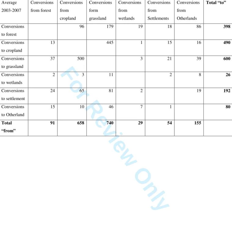
According to the information contained in the 2009 GHG inventory reports, the total area reported 4

under a “land-use change” category in EU-25 was about 380,000 km2 for the year 1990 and 352,000 5

km2 for the year 2007, i.e. slightly decreasing over time (Table 2). When considering the time a land 6

remains in the conversion status (20 years for most countries), approximate values of LUC annual rates 7

may be estimated (Table 2, average for the period 2003-2007). About 17,800 km2 undergo a land-use 8

change every year within EU-25, representing a small fraction (0.41%) of the total area. Additionally, it 9

is estimated that about 4300 km2 are annually converted to forest in the European part of the Russian 10

Federation, Belarus and Ukraine. 11

12

The gross fluxes from LUC at European level are summarized in Fig. 3. The carbon balance associated 13

with LUC is a net sink of 1.5 Tg C yr-1 for EU-25 and reaches 9.6 Tg C yr-1 when data from European 14

Russia, Belarus and Ukraine are also considered (a sink of 9.0 Tg C yr-1 due to conversion to forest and 15

a source of 0.9 Tg C yr-1 due to deforestation reported in European Russia). These numbers include 16

average emissions during 2003-2007 due to LUC that occurred up to 20 years before, depending on the 17

methods used by each country. 18

19

The net small sink from LUC at the European level masks large fluxes of opposite signs between 20

different land-use types. For instance, at EU-25 level one can see that the largest single LUC-induced 21

gross area change is the conversion of croplands to pasture (5000 km2 yr-1), which sequestered 11 Tg C 22

yr-1 carbon. But this transition is offset elsewhere by about 4400 km2 yr-1 of grasslands being ploughed 23

for crop cultivation, which causes a net loss of carbon to the atmosphere of nearly 10 Tg C yr-1. At the 24

European level, the largest single flux occurs in lands converted to forests (a sink of 18.3 Tg C yr-1). 25

Part of this sink is balanced by carbon loss by deforestation (7.3 Tg C yr-1). If the absolute values of all 26 3 4 5 6 7 8 9 10 11 12 13 14 15 16 17 18 19 20 21 22 23 24 25 26 27 28 29 30 31 32 33 34 35 36 37 38 39 40 41 42 43 44 45 46 47 48 49 50 51 52 53 54 55 56 57 58 59 60

For Review Only

LUC are summed up, it results in a total flux of 50 Tg C yr-1 induced by LUC at the European level. As 1

many countries do not yet report all LUC to UNFCCC, this estimate is likely to be underestimated. The 2

analysis indicates that despite the net carbon balance of all land-use changes being small, and despite 3

the fact that the LUC areas are usually very small compared to total area, regionally the LUC can be 4

very important, corresponding to a very high NBP of positive or negative sign. 5

6

When interpreting the data on LUC in Table 2 and Fig. 3 it is important to note that differences may 7

occur among countries in terms of: (i) completeness of reporting (while most countries report 8

conversions to forests and many report conversions from/to cropland and grasslands, conversions from 9

other land uses are reported less frequently); (ii) reported time series (e.g. most countries use the 20 10

year default transition period, but some countries have data only since1990); (iv) coverage of carbon 11

pools (e.g. many countries do not report fluxes from forest soils); (iii) land use definition (e.g. some 12

lands may be classified either under cropland or grassland, depending on the country’s definitions); (v) 13

methods to estimate carbon stock changes (in some case the spatiotemporal variability of soil carbon 14

and biomass is explicitly considered, but in other cases only default IPCC emission rates are used). 15

Moreover, some basic data are unknown, such as for instance, the fate of carbon in settlements. When 16

buildings are constructed, whether soil carbon buried under concrete isolated from the atmosphere, or 17

decomposed by microbes and quickly lost to the atmosphere will change the sign of the carbon balance 18

of new settlements. At face value, gardens are productive and fertilized lands, which may be 19

overlooked and yet are a significant carbon sink given the total urban and peri-urban area, which is 20

about 7% of total land area. Despite these limits, the data from countries’ GHG inventories are 21

presently the best data available for LUC-induced carbon flux estimates. 22

23

Obviously, net land-use change has no major effect on the trace gas cycle of Europe. Land-use intensity 24

and the associated emissions from fertilizer application and meat production is more important than 25 land-use change. 26 3 4 5 6 7 8 9 10 11 12 13 14 15 16 17 18 19 20 21 22 23 24 25 26 27 28 29 30 31 32 33 34 35 36 37 38 39 40 41 42 43 44 45 46 47 48 49 50 51 52 53 54 55 56 57 58 59 60

For Review Only

1

7. Where does the excess carbon dioxide and nitrous oxide go?

2 3

Figure 3 shows an export of CO2 and N2O out of the European domain, and the question emerges:

4

Where do these reactive and non-reactive trace gases go, and what area outside Europe would be 5

needed to assimilate this surplus? This would be the trace gas footprint of Europe. 6

7

Assuming that CO, CH4, NH3, and NOx are deposited in Europe, N2O and CO2 remain as the major

8

trace gases being exported to other regions of the globe. 9

In total, Europe exports 0.4 Tg N2O-N yr-1. Assuming an uptake in forest equivalent to Europe of about

10

2 g N2O-CO2-C-eq m-2 yr-1, the Siberian forests extending over 12.80 1012 m2 (Shvidenko & Nilsson,

11

1994) would assimilate only about 20% of this excess, the remaining could interact with volatile 12

organic carbon, would be mixed across the globe, or enter into the stratosphere. 13

14

The excess CO2 of 1294 Tg yr-1 could be absorbed by oceans or the biosphere or add to the atmospheric

15

increase in CO2. According to Canadell et al. (2007) we may assume that 23% enters into the oceans,

16

and 38% remains in the atmosphere. 39% or 504 Tg yr-1 is expected to be absorbed by vegetation of 17

neighbouring continents. We may take Siberia as one candidate for this footprint. Shvidenko and 18

Nilsson (2002) estimate a carbon sequestration rate for Siberian forest of 210 Tg C yr-1 and an 19

additional 50 Tg C yr-1 may enter into soils (Shvideno & Nilsson, unpublished). Thus, the Siberian 20

forest may re-assimilate 20% of the excess European CO2-C, leaving about 244 Tg yr-1 to be

21

assimilated in other regions. In any case, the European footprint on the global terrestrial surface may be 22

twice as large as Siberia. 23 24 8. Conclusions 25 26 3 4 5 6 7 8 9 10 11 12 13 14 15 16 17 18 19 20 21 22 23 24 25 26 27 28 29 30 31 32 33 34 35 36 37 38 39 40 41 42 43 44 45 46 47 48 49 50 51 52 53 54 55 56 57 58 59 60

For Review Only

The carbon cycle shows a significant distortion from human impacts. We are extracting 30% of the 1

carbon flow as harvest, which reduces the amount that could be stored in soils. The carbon balance of 2

soils (excluding the carbon storage in forest biomass) is still a minor carbon sink. However, studying 3

only the carbon cycle is not sufficient, if a mitigation of the global warming potential is anticipated. Not 4

only greenhouse gases, but also non-greenhouse gases interact, mostly offsetting the apparent terrestrial 5

sink. Although CO2 from fossil fuel burning remains the most important greenhouse gas added into the

6

atmosphere by human activity, CH4, N2O and CO contribute almost 50% to the total European global

7

warming potential, and about 75% of this input originates from agriculture. Including these emissions 8

of greenhouse gases, the European soils are a net source. 9

10

The human impact on the carbon cycle is significant and occurs everywhere. Harvest exceeds NBP by 11

threefold, which means that more carbon is extracted from the natural carbon cycle than it is remaining 12

in soils. Total harvest takes about 30% of NPP, but 10% of this is the hidden cost of production. On the 13

other hand, growth of vegetation is stimulated by atmospheric nitrogen deposition. 50% of forest NBP 14

and harvest could be due to the anthropogenic input of atmospheric nitrogen. 15

16

Europe creates an excess of N2O and CO2, which is re-assimilated on other continents, in the ocean or

17

remains in the atmosphere. For the excess CO2 a land surface of at least twice the size of Siberia would

18

be needed to compensate European emissions and ensure no net contribution to the global carbon 19

balance (no climate mitigation). Obviously, Europe has a long way to go to reach climate neutrality. 20

21

What are the implications of these findings for climate change mitigation? Reducing fossil fuel burning 22

still remains the prime target for climate mitigation. However, given the large emissions from croplands 23

and grasslands including in-house livestock, and the still increasing intensity of land-use, a strong effort 24

will also be needed from agriculture. Thus, additional measures must be taken, to restrict fertilizer use 25

according to site conditions and the types of crops, reduce the organic and mineral fertilizer input in 26 3 4 5 6 7 8 9 10 11 12 13 14 15 16 17 18 19 20 21 22 23 24 25 26 27 28 29 30 31 32 33 34 35 36 37 38 39 40 41 42 43 44 45 46 47 48 49 50 51 52 53 54 55 56 57 58 59 60