Experimental investigation of transitional flow in a toroidal pipe

(1)

doi:10.1017/jfm.2013.603

Experimental investigation of transitional flow

in a toroidal pipe

J. Kühnen1,2,_†_{, M. Holzner}3_{, B. Hof}2,4 _{and H. C. Kuhlmann}1

1_{Institute of Fluid Mechanics and Heat Transfer, Vienna University of Technology,}

Resselgasse 3/1/2, A-1040, Vienna, Austria

2_{IST Austria, Am Campus 1, 3400 Klosterneuburg, Austria}

3_{Institute of Environmental Engineering, ETH Z¨urich, Wolfgang Pauli Strasse 15, CH-8093 Z¨urich,}

Switzerland

4_{Max Planck Institute for Dynamics and Self Organization, Bunsenstrasse 10, D-37073 G¨ottingen,}

Germany

(Received 28 February 2013; revised 20 September 2013; accepted 7 November 2013; first published online 13 December 2013)

The flow instability and further transition to turbulence in a toroidal pipe (torus) with curvature ratio (tube-to-coiling diameter) 0.049 is investigated experimentally. The flow inside the toroidal pipe is driven by a steel sphere fitted to the inner pipe diameter. The sphere is moved with constant azimuthal velocity from outside the torus by a moving magnet. The experiment is designed to investigate curved pipe flow by optical measurement techniques. Using stereoscopic particle image velocimetry, laser Doppler velocimetry and pressure drop measurements, the flow is measured for Reynolds numbers ranging from 1000 to 15 000. Time- and space-resolved velocity fields are obtained and analysed. The steady axisymmetric basic flow is strongly influenced by centrifugal effects. On an increase of the Reynolds number we find a sequence of bifurcations. For Re = 4075 ± 2 % a supercritical bifurcation to an oscillatory flow is found in which waves travel in the streamwise direction with a phase velocity slightly faster than the mean flow. The oscillatory flow is superseded by a presumably quasi-periodic flow at a further increase of the Reynolds number before turbulence sets in. The results are found to be compatible, in general, with earlier experimental and numerical investigations on transition to turbulence in helical and curved pipes. However, important aspects of the bifurcation scenario differ considerably.

Key words:instability, transition to turbulence

1. Introduction

Transition to turbulence in straight circular pipes is one of the oldest and most fundamental problems of fluid mechanics, entailing various fundamental questions about the nature of turbulence (Eckhardt 2008). The understanding of the physics of transition to turbulence in straight pipes has experienced significant progress in recent years due to the application of modern optical measurement techniques and computationally based theoretical modelling (Hof et al. 2004; Eckhardt et al. 2007; Mullin 2011). It is a characteristic of straight pipe flow that transition occurs

† Email address for correspondence: [email protected]

https:/www.cambridge.org/core

. University of Basel Library

, on

30 May 2017 at 21:24:59

, subject to the Cambridge Core terms of use, available at

https:/www.cambridge.org/core/terms

.

(2)

in spite of the linear stability of the laminar Hagen–Poiseuille flow if the flow perturbations exceed a certain threshold. Moreover, and unlike plane Poiseuille flow, Rayleigh–B´enard convection, or Taylor–Couette flow, there exists no instability of Hagen–Poiseuille flow for any Reynolds number Re = Ud/ν, where U is the mean velocity, d is the diameter of the tube and _{ν is the kinematic viscosity of the} fluid (Drazin & Reid 1981). Consequently, turbulence can only be triggered by finite amplitude perturbations. Following Reynolds (1883) the critical point is then defined as the Reynolds number above which turbulence is first sustained indefinitely, whereas below it, any turbulence initially in the flow will eventually decay. As shown by Avila et al. (2011) this critical Reynolds number is Rec≈ 2040, where the decay of turbulence is balanced by a spreading process.

In curved pipes the process of transition to turbulence differs qualitatively from that in straight pipes. Curved-pipe flow has received less attention than straight-pipe flow, even though the former is of no less importance: practically all pipes in nature, e.g. blood vessels, or in engineering are curved. In curved pipes the basic flow is strongly affected by an imbalance between the cross-stream pressure gradient and the centrifugal force, which leads to a secondary cross-stream motion, typically in the form of a pair of steady streamwise Dean vortices symmetric with respect to the tangent plane. With increasing Dean number the maximum of the streamwise velocity is shifted radially towards the outer wall of the pipe. Owing to the increased gradient of the streamwise flow, the drag in curved pipes is considerably higher than in straight pipes. For reviews of curved-pipe flow and further reading, we refer to Berger, Talbot & Yao (1983), H¨uttl & Friedrich (2000, 2001), Naphon & Wongwises (2006) and Vashisth, Kumar & Nigam (2008).

Dean (1927, 1928) has solved the simplified Navier–Stokes equations for a coiled pipe of small curvature showing that the flow is governed by two parameters. These parameters are the curvature ratio _{δ = d/D of the pipe diameter d to the coiling} diameter D, and the Dean number De = Re√δ. Taylor (1929), White (1929) and Adler (1934) found that the flow in curved pipes remains laminar up to Reynolds numbers higher at least by a factor of two than in straight pipes. They also noticed that transition to turbulence is not as abrupt as in straight pipes but occurs gradually, without any discontinuity of the characteristic observables such as the pressure drop. Sreenivasan & Strykowski (1983) investigated curved-pipe flow for moderate Reynolds numbers. They found that the turbulent flow in a straight pipe becomes laminar after entering a coiled pipe of the same diameter. They recognized, moreover, that the curved-pipe flow becomes time-periodic before turbulence commences. The oscillation amplitude was found to be strongest near the inside wall of the pipe.

Webster & Humphrey (1993) investigated the unsteady three-dimensional flow through a helical pipe at transitional conditions using laser Doppler velocimetry (LDV). For _{δ = 0.055 they measured the onset of periodic low-frequency perturbation} waves at Rec= 5060. They specified the non-dimensional frequencies found with fd_{/U = 0.25 and 0.5 for all Reynolds numbers investigated. Complementary numerical} simulations of Webster & Humphrey (1997_{) for Re = 5480 were in agreement with}

the experimental results of Webster & Humphrey (1993). Dye streaks, used for visualization, were found to diffuse at Re = 6330. Webster & Humphrey (1997) interpreted this behaviour as the onset of turbulent fluctuations.

Flows in weakly curved ducts with constant curvature and in helical pipes with small torsion have a common asymptotic limit: toroidal-pipe flow. However, the inlet and outlet conditions are generally different. Piazza & Ciofalo (2011) numerically simulated the flow in a circular toroid with a circular cross-section driven by a

, on

30 May 2017 at 21:24:59

.

(3)

constant streamwise body force, using periodic boundary conditions. For _{δ = 0.3 a} supercritical Hopf bifurcation was found in the interval 4556< Rec1< 4605, giving rise to an azimuthally travelling wave which took the form of a varicose streamwise modulation of the two Dean vortex rings. The wave was described as mainly affecting the Dean vortices but not the boundary layers on the wall. For 5042< Rec2< 5270, a secondary Hopf bifurcation was discovered leading to a quasi-periodic flow. The second wave, created for Re> Rec2, arises as an array of oblique vortices localized in the two boundary layers of the basic flow at the edge of the Dean vortex regions. The oscillatory perturbation flows in both the periodic and the quasi-periodic regimes were anti-symmetric with respect to the equatorial midplane of the torus for _{δ = 0.3. For} δ = 0.1, Piazza & Ciofalo (2011) found a direct transition from a steady to a quasi-periodic flow between 5139< Re < 5208, associated with hysteresis. The travelling waves for _{δ = 0.1 were symmetric with respect to the equatorial midplane of the torus.}

Like Cioncolini & Santini (2006), most studies on curved-pipe flow aimed at reliable pressure-drop correlations, because the friction factor is an important quantity for industrial design. Moreover, all experimental studies on transition to turbulence in fully developed curved pipes have been conducted in helical pipes with a small pitch. While the closed flow in a torus considered by Piazza & Ciofalo (2011) offers a perfect geometry for theoretical and numerical investigations, experiments using a torus are difficult, because the driving pressure gradient cannot be imposed as easily as in open systems. Apart from Madden & Mullin (1994), del Pino et al. (2008) and Hewitt et al. (2011), who experimentally studied the transient flow in a torus during spin-up from rest and spin-down from solid-body rotation, we are not aware of any other experimental work on the flow in a torus.

In the present work we experimentally investigate the flow and its instability in a torus by means of visual observations, high-speed stereoscopic particle image velocimetry (SPIV) and pressure drop measurements. Particular attention is paid to the detection and investigation of travelling waves. To that end an experiment was set up where the flow inside a torus is driven by a moving sphere. For a sufficiently large aspect ratio (circumference-to-pipe-diameter ratio) the perturbations induced by the sphere remain localized, and bulk flow properties can be measured which are independent of the particular driving. We measure the full three-dimensional and time-resolved structure of the transitional flow including all three velocity components over the entire length and cross-section of the pipe.

2. Experimental setup

2.1. The facility

The toroidal pipe is realized as a toroidal cavity (torus) in a stationary block of Perspex (polymethyl methacrylate). A ferromagnetic sphere, which is actuated by a strong magnet from the outside, is put into the toroidal cavity to drive the flow in the cavity. The main components and the driving mechanism of the experiment are sketched in figure 1. The stationary block is made of two highly transparent and polished Perspex disks into which a circular groove of semi-circular cross-section has been machined, concentric with the disks. The two disks are mounted mirror-symmetrically. The two grooves in the disks hence form a closed toroidal cavity, i.e. a curved tube which is to be filled with the working fluid. To drive the fluid motion a ferromagnetic stainless chromium steel sphere with diameter slightly less than the toroidal tube is placed in the toroid. The steel sphere is actuated from outside the toroidal cavity using a strong permanent magnet mounted on a rotating boom. To

, on

30 May 2017 at 21:24:59

.

(4)

7 6 5 4 3 2 1 d

FIGURE1. Assembly drawing (side view) of the experimental setup. Lower (1) and upper (2) Perspex disk are bolted (3) and sealed using a 2.5 mm rubber O-ring (4) in a 2_{.2 mm×2.5 mm} groove. A total of 32 screws (16 outside and 16 within the torus groove, at an angular distance of π_{/8) are used to ensure leak-proof tightness. A flat pot magnet (5) with a threaded stem} is incorporated into the boom (6) just below the centreline of the tube, leaving an adjustable distance of 1 mm to the lower Perspex disk. The boom is rotated around the shaft (7) by a geared direct current motor (not shown). The diameter of the torus is D = 614 mm, and the diameter of the tube is d = 30.3 mm. Drawing not to scale.

achieve a constant and precisely adjustable flow rate in the torus the boom is rotated at a constant angular velocity, thereby steadily moving the sphere inside the torus, driving the fluid motion. The driving system to rotate the shaft consists of an electric gear motor combined with a belt drive (neither are shown in figure 1). The Reynolds number is defined as Re = Ud/ν, where d is the diameter of the tube, ν is the kinematic viscosity of the fluid, and the bulk velocity U = ΩD/2 with angular velocity Ω of the rotating boom and D the diameter of the centre circle of the torus.

When measuring flow details with SPIV, a large tube diameter d is desirable. Therefore, a tube diameter of d = 30.3 mm was chosen, slightly larger than the diameter of the sphere ds = 30 mm, to permit rolling motion of the sphere. This left a small sickle-shaped gap of maximum 0.3 mm at the upper half between torus wall and sphere. The total area of the gap is Agap= 14.2 mm2 corresponding to 1.9 % of the tube’s cross-section. Through the gap between sphere and tube wall a small leak flow will arise. When the fluid in the torus has reached a constant velocity after spin up from rest, the sphere only has to balance the minor friction losses in the tube, which amounted to e.g. ≈20 Pa at Re = 5000.

Since we are interested in a small curvature ratio _{δ, a large diameter D of the torus} is preferable. We used a centreline diameter of D = 614 mm, resulting in a curvature ratio _{δ = d/D = 0.049. This corresponds to a large aspect ratio (circumference to tube} diameter) of _{Γ = π/δ − 1 ≈ 63. To achieve a surface finish of the tube comparable} to that of glass pipes, the Perspex surface was polished. The torus dimensions including the manufacturing tolerances are D = 614±0.1 mm and d = 30.3±0.03 mm, respectively.

According to the manufacturer’s specification the pot magnet had ≈216 N adhesive force perpendicular to the surface to which the magnet should stick (equivalent to 22 kg bearing capacity). However, the actual adhesive force decreases quickly with increasing distance and is also influenced by the alloy of the object of magnetic attraction. Since the minimum distance between magnet and sphere in the setup is

, on

30 May 2017 at 21:24:59

.

(5)

≈5 mm (see figure 1_{), the actual adhesive force imposed on the sphere is ∼0.49 to}

0.98 N (0.05 to 0.1 kg) according to the specification. This was found sufficient to control the sphere in the liquid-filled torus. Owing to the high inertia of the rolling sphere compared to any forces caused by the flow fluctuations the sphere would always roll very smoothly and accurately follow the magnet. Observations of the sphere by a camera mounted on the boom did not allow detection of any relative motion between the sphere and the magnet, once the steady rolling motion was established. Only in the case of very fast or jerky acceleration or deceleration would the sphere not follow the magnet and lose the magnetic bond.

To detect the temperature of the fluid in the torus, two small Platinum SMD Flat Chip temperature sensors (Vishay Beyschlag, PTS 0603, 100) are used. Every sensor is mounted on the front end of a bracket pin with a diameter of 2 mm. The bracket pins are plugged into holes drilled into the upper Perspex disk at an angular distance of π/2, just above the upper apex of the tube. The holes do not quite push through into the toroidal volume but leave a thin indentation of approximately 0.08 mm between the temperature sensors and the fluid in the torus. For data acquisition the two sensors are connected to a Validyne UPC 2100 PCI sensor interface card. The mean value of the two sensor signals, averaged over 20 s, is used to determine the temperature of the fluid in the torus with an accuracy of ±0.1 K. The ambient temperature in the laboratory could vary slowly by approximately ±2 K during each day. As individual measurements would never take longer than 5 min, no additional measures were taken to control the temperature of the fluid. To eliminate problems due to the differing refractive indices such as unwanted displacement, hidden regions and multiple images (Lowe & Kutt 1992), arising for objects placed inside containers with cylindrical walls, a refractive-index-matched mixture of distilled water and ammonium thiocyanate was used as the working fluid (Budwig 1994; Hopkins et al. 2000). The kinematic viscosity ν of the index-matched fluid as a function of temperature was determined by means of a Schott Cannon-Fenske capillary viscometer. For temperatures ranging from 20 to 30◦_{C the kinematic viscosity of the} index-matched fluid was approximated by the fourth-order polynomial

ν = 4.5 × 10−7_{+ 2.7 × 10}−7_{T − 1.8 × 10}−8_T2_{+ 4.9 × 10}−10_T3_{− 4.9 × 10}−12_T4_, (2.1) which was fitted to the measured data by least squares. Here, T is measured in degrees Celsius and _{ν in m}2 _s−1_{. A combination of a LabView program and a system} consisting of a controller unit (LSC 30/2, 4-Q-DC, Maxon Motor AG), a USB data acquisition card (National Instruments 6008) and direct current motor (RE 25, Maxon Motor AG) with speedometer (DCT 22) and planetary gear (GP 32) was used to set and continually control the Reynolds number. The LabView program contained the functional relationship between temperature, viscosity and the geometrical data based on which the required angular velocity of the sphere for a specified Reynolds number was calculated and implemented. Optionally, an automatic mode can be used to increase or decrease the Reynolds number stepwise by predefined step sizes and at predefined times. The setup provided the possibility of investigating the flow in the torus for adjustable Reynolds numbers ranging from 1000 to 15 000 with an accuracy of ±2 %, taking into account the leak flow past the sphere (see §3.1.3).

2.2. Measurements

For preliminary investigations and visual identification of pertinent flow structures, the fluid was seeded with glitter particles (polyester glitter, Sigmund Lindner GmbH)

, on

30 May 2017 at 21:24:59

.

(6)

1 2 3 4 6 5 d

FIGURE 2. (Colour online) Sketch (side view) of the stereoscopic PIV system. To reduce optical reflections, a prism is placed on the upper Perspex disk of the torus: lower Perspex disk (1), upper Perspex disk (2), screws (3), prism (4), light sheet (5), cameras (6). A few drops of glycerine were used to create a thin film between the upper Perspex disk and the prism, enabling seamless contact. Drawing not to scale.

which reflect light and make the flow structure visible. However, visibility was limited because the particles tended to get stuck in the gap between the sphere and the torus wall, and would hence block the sphere if their concentration was too high. Therefore, only a limited number of particles could be used. Still photographs as well as video recordings were made with a Nikon D 7000 DSLR camera. Movies of the flow structures were recorded with a frame size of 1920 × 1080 pixels at 24 f.p.s. For the video recordings the camera was mounted on an additional boom which rotated at the same speed as the boom driving the sphere. This allowed observations in the frame of reference rotating with the angular velocity of the sphere, which nearly equals the mean flow velocity U.

The pressure drop between two pressure holes (bore holes with an internal diameter of 1 mm) was determined using a differential pressure sensor (Validyne DP103, ultra low-range wet–wet differential pressure transducer). The pressure transducer was calibrated using a Betz manometer and it had a full range of 140 Pa with an accuracy better than 0.35 Pa. The pressure holes were located at the top of the upper side of the tube. The sampling rate was 10 ms.

A SPIV system from LaVision was used to measure the three components of the velocity vectors over a cross-section perpendicular to the flow. It consisted of a pulsed Quantronix Darwin Duo laser (diode pumped Nd:YLF laser, wavelength 527 nm, 60 mJ total energy) and two Phantom V10 high-speed cameras with a full resolution of 2400×1900 pixels. The temporal resolution was set to 100 Hz. Silver-coated hollow glass spheres (S-HGS-10, mean diameter 10 µm, _{ρ = 1.4 g cm}−3_{, Dantec Dynamics)} were used as seeding particles.

Previous investigators (see e.g. van Doorne & Westerweel 2007) have demonstrated the possibilities and potential of SPIV in investigating and capturing the appearance and development of transitional flow in a pipe. The same principle is applied in the experimental setup used for this work. Figure 2 provides a sketch of the setup which was used for stereoscopic PIV, showing the arrangement of Perspex disks, the light sheet and two cameras in a 45◦ _{viewing angle. Due to the 45}◦ _{viewing angle the}

, on

30 May 2017 at 21:24:59

.

(7)

light would be refracted at the outer wall of the Perspex disk, which would reduce the effective viewing angle of the cameras and degrade the image quality. Therefore, a prism made of Perspex is attached to the upper Perspex disk such that the optical axis is perpendicular to the air–Perspex interface.

The calibration target, needed for the calibration of the SPIV measurements, was custom-built by Die Signmaker GmbH (G¨ottingen). It consisted of a 5 mm lattice of black dots with a diameter of 1 mm printed on both sides of a 1.5 mm Perspex disk with a cross-sectional diameter of 30 mm, i.e. slightly less than the tube diameter. The disk was kept in position (congruent with the light sheet of the laser) for the calibration procedure by a tiny locking screw drilled into the torus wall. After the calibration images were shot, the screw was removed and the calibration target was released. The experimental setup was too sensitive to be disassembled after calibration, as dismantling and repeated assembly would have caused small displacements and hence spoiled the calibration. Therefore, the disk was just left in the torus and went with the flow. After a few turns of the actuator the disk would then be located in front of the sphere, not perturbing or changing the flow far from the sphere in addition to the perturbations induced by the actuator itself.

The evaluation of the 3D-vector fields from the PIV images was performed with commercial PIV software (DaVis 8, LaVision). The interrogation area was 32 × 32 pixels with an overlap of 50 %. The maximum particle displacement between two frames was approximately 11 pixels in the horizontal direction and 8 pixels in the vertical direction. Subsequently, the acquired data were analysed with MathWorks MATLAB R2011b, which was used as programming environment.

A fibre-flow 2D-LDV system by Dantec Dynamics was employed for laser Doppler velocimetry measurements. From the LDV data we obtained spectra of the streamwise velocity at single points within the cross-section of the pipe. The average sampling rate was 200 Hz.

3. Results

Most of the space-resolved measurements are taken in a meridional cross-section of the torus. Therefore, we use local Cartesian coordinates (x, y, z) as shown in figure 3, where (u, v, w) are the respective Cartesian velocity components. The x-axis is directed radially inward towards the centre of the torus. Figure 3 also sketches characteristic cross-stream flow structures of the basic steady flow, where we use the same notation as Webster & Humphrey (1997). The steady basic flow is mirror-symmetric with respect to the equatorial plane y = 0. In a wide core region around the axis y = 0 the cross-stream flow is directed radially outward in the negative x-direction from the low-speed core region (ls) to the high-speed core region (hs) of the streamwise velocity. The cross-stream flow returns radially inward in two symmetrically located wall jets called cross-stream wall layers. The thickness of these wall jets grows as they turn inward. Before reaching the inner equatorial point C the jets turn sharply in region I and merge to form the core flow in the low-speed region directed radially outward.

3.1. Evaluation of the experimental setup

We are interested in the toroidal pipe flow driven by a prescribed steady volume flux. Due to the particular driving by a moving sphere the ideal flow is perturbed in the vicinity of the sphere. To assess the extent to which the flow field in the torus can be considered fully developed, i.e. stationary and independent of the driving mechanism,

, on

30 May 2017 at 21:24:59

.

(8)

x y A B C D hs Core ls Region I Cross-stream wall layer

Outer equatorial point Inner equatorial point

FIGURE 3. Salient flow structures in a cross-section of the toroidal pipe and notation. A Cartesian (x, y, z) coordinate system is used in the meridional observation plane at constant toroidal angle ϕ. The poloidal (meridional) angle is α. The x-axis is directed toward the symmetry axis of the torus. The abbreviations hs and ls denote regions of high-speed and low-speed streamwise velocity, respectively. A, B, C and D denote the north pole (B), south pole (D), outer equatorial (C) and inner equatorial (A) points.

the effect of the rolling sphere on the flow has to be evaluated. The perturbations arise in the form of an entrance-length effect and a leakage through the gap between the sphere and the torus. As the curvature ratio is constant throughout this work, the strength of the flow is measured using the Reynolds number instead of the Dean number.

3.1.1. Entrance-length effect

If the sphere moved as a plug with constant velocity without rolling, a pure streamwise and steady velocity field would be enforced at the surface of the sphere. Due to the imposed velocity on the semi-spherical end wall and the velocity discontinuity along the line of contact, there exists a return flow in the frame of reference moving with the sphere which represents a perturbation to the fully developed toroidal-pipe flow decaying away from the sphere. In operation the sphere is rolling in the torus. While the rolling motion prevents any perturbation of stick–slip type and thus adds to keeping the translational velocity constant, provided the rotation rate of the beam is constant, the rolling motion induces an additional cross-stream velocity component which will also decay away from the sphere under subcritical conditions.

To quantify the decay of the above perturbations we measured the streamwise velocity w as a function of the distance from the sphere using SPIV. Figure 4

shows the result as a function of time (related to the distance from the sphere by ¯U) for Re = 3600, Re = 4300 and Re = 4700 in the centre of region I at the point (x, y) = (0.17 d, 0.31 d). This point has been selected because the flow instability can be measured sensitively in this region. A period of 12 s is shown, equivalent to approximately one full revolution of the sphere around the torus. At Re = 3600 (figure4a) the flow is fully developed, except for the immediate vicinity of the sphere where the streamwise velocity component varies strongly. At some distance from the sphere the measured velocity w is constant up to small fluctuations, which are mainly due to the noise of the PIV data. Excluding the range disturbed by the sphere, the r.m.s. value of the streamwise velocity is 0_{.78 % of the mean value.}

, on

30 May 2017 at 21:24:59

.

(9)

(a) (b) (c) w (m s –1) w (m s –1 ) w (m s –1 ) z (m) Perturbed Analysed t (s) 0.1 0.2 0 0.1 0.2 0.3 0 0.1 0.2 0.3 0 –1.5 –1.0 –0.5 0 0 –8 –6 –4 –2 2 –1.5 –1.0 –0.5 0 0.5 0 –8 –6 –4 –2 2 4 0 0.5 1.0 –1.5 –1.0 –0.5 0 –6 –4 –2 2 4

FIGURE 4. Time traces of the streamwise velocity w at (x, y) = (0.17 d, 0.31 d) for Re= 3600, Re = 4300 and Re = 4700 as a function of time t (bottom axis) and azimuthal length z (top axis). A typical PIV run of 12 s, comprising approximately one full revolution of the sphere, is displayed. The coordinate origin was defined by the transit of the sphere. The vertical dotted lines are drawn with a spacing of _{1ϕ = π/2. The velocities of the sphere are} Us= 0.19 (a), 0.22 (b) and 0.24 (m s−1) (c).

At Re = 4300 (figure 4b) a very distinct sinusoidal modulation of the streamwise velocity is observed, which differs markedly from the signature of the wake flow. With the centre of the sphere at _{ϕ = 0, the oscillation amplitude is nearly constant} in a certain region around _{ϕ = π. To analyse the oscillatory flow in the bulk we} consider only a time interval of 2.25 s corresponding to 0.5 m or 'π/2, which leaves a sufficient safety margin from the region disturbed by the sphere. This range is

, on

30 May 2017 at 21:24:59

.

(10)

E (m 2s –2 ) t (s) Disturbed 0 0.5 1.0 1.5 2.0 2.5 3.0 1 2 3 (× 10–4₎

FIGURE 5. (Colour online) Transit of the sphere through the measurement plane for Re= 3600. The spatially averaged (over x and y) kinetic energy of the velocity fluctuations is displayed in the direct vicinity of the sphere. The streamwise_(Ek

kin), cross-stream (Ekin⊥) and total fluctuation energies Ekin= Ekink + Ekin⊥ are shown.

marked as ‘Analysed’ in figure 4(b) and it is typically located on the side of the torus opposite to the sphere. At Re = 4700 a dominant frequency can still be recognized, but the amplitude is no longer constant.

To confirm that the perturbations induced by the rolling sphere are spatially restricted, we consider the kinetic energy. Decomposing the velocity field into a temporal mean and a fluctuation part u = ¯u + u0_{, we define the streamwise and} cross-stream fluctuation energies E_k _{= hw}02_{i and E}

⊥= hu02i + v02, respectively, where the brackets indicate averaging over the _{(x, y)-plane. Figure} 5 shows that the range of perturbed flow is confined to the vicinity of the sphere as indicated by the arrows, while further away from the sphere the kinetic energy of the fluctuations is nearly constant and very small. For Re = 3600 the flow is perturbed for ≈2.4 s during the passage of the sphere, corresponding to an azimuthal angle of 0_{.46π slightly} asymmetric about the location of the sphere. It is concluded that there exists a range of fully developed flow which is nearly unperturbed by the details of the flow around the rolling sphere.

As the Reynolds number increases, the unperturbed range decreases. Based on an extrapolation of the measured length of the zone disturbed by the sphere at low and moderate Reynolds numbers the length of the zone of the nearly fully developed bulk flow for Re = 6000 is at least 15 % of one full revolution of the torus. This range is predicted at _{ϕ ∈ [0.85π, 1.15π] relative to the sphere at ϕ = 0. Even though the} lengths of the wakes upstream and downstream from the sphere differ, we selected a symmetric region for simplicity, leaving a sufficient safety margin to the perturbed regions. All data analysed were taken from these unperturbed angular sections.

3.1.2. Plunger with sphere

To assess the effect of the rolling of the sphere on the end-wall-induced perturbations and possibly on the bulk flow, the driving was modified. Instead of simply a sphere, a plunger was used, made from polyoxymethylene (POM) (figure 6). The plunger was machined in the form of a slightly modified cylindrical block with a diameter of 30.1 mm, by which the total area of the gap was reduced to 9_{.49 mm}2 _or 1.3 % of the tube’s cross-section.

A bore of 20 mm diameter was drilled into the plunger, providing space for a steel sphere with 18 mm diameter. This steel sphere was also controlled by the magnet from

, on

30 May 2017 at 21:24:59

.

(11)

Pipe walls

Plunger

Sphere

Flow direction

FIGURE 6. (Colour online) Sketch of the first type of plunger within the torus. A small sphere of ds= 18 mm placed inside the plunger is used as the object of magnetic attraction to move it. Only the streamwise moving walls of the plunger, instead of the surface of the rolling sphere, interact with the flow in the torus.

outside, but its rolling motion would not influence the flow in the torus. As the plunger was cylindrical, its shape did not perfectly match the slightly curved torus. Due to the lubrication of the fluid between the two solid surfaces of tube and plunger, the plunger would slide through the tube very well without excessive stresses or seizures at the wall. Only very mild wear, mostly originating from the tracer particles in the fluid, was noticed.

We found that the design type of the actuator had very little influence on the length of the perturbation flow near the moving end wall and no influence on the bulk flow. For that reason only a rolling sphere was used for all measurements.

3.1.3. Leak flow past the sphere

The azimuthal velocity Us of the centre of the sphere is precisely known as it is controlled by the angular velocity Ω of the rotating boom. Comparing the associated flow rate Usπd2/4 with the measured flow rate allows us to determine the leak flow past the sphere. The actual mean velocity in the torus U was determined in two ways. First, the pressure drop _{1p over the angle 1ϕ = π/2 was measured. The result} was compared to pressure-drop data obtained from published correlations of White (1929), Hasson (1955) and Mishra & Gupta (1979) for the laminar regime, which all deviate less than 1.5 %. Up to Re . 2500 we find excellent qualitative agreement with these correlations but a practically constant deviation which can be attributed to a slightly slower velocity of the fluid U than the azimuthal velocity Us of the sphere by ≈3 %. In addition, U was obtained from SPIV measurements. The resulting leak flux amounted to 3 % of the actual mean volume flux, consistent with the flow rate from the pressure drop. Therefore, we can safely determine the mean velocity as U = 0.97 Us. It must be noted, however, that a slightly nonlinear behaviour of the leak flow for increasing Reynolds number could not be ruled out.

3.2. Velocity-field measurements 3.2.1. Steady basic flow

In the following the flow field in the bulk is considered, which is practically unaffected by the end-wall perturbations. For small Reynolds numbers the flow field is unique and steady. For Re = 3600 the steady basic flow has developed its characteristic structure which is caused by the pipe curvature. The velocity field measured by SPIV in the entire cross-section is shown in figure 7. As the fluid in the core region is centrifugally driven toward the outer wall, the maximum streamwise velocity is located in the plane of symmetry and near the outer wall. Therefore, the gradient of the

, on

30 May 2017 at 21:24:59

.

(12)

0.1U 0 0.2 0.4 0.6 0.8 1.0 1.2 1.4 1.6 0 – 0.5 0.5 – 0.5 0.5

FIGURE7. (Colour online) Entire cross-sectional flow field of the tube in the steady laminar regime (at Re = 3600). Streamwise (colour contours) and in-plane velocity (vectors), both normalized with the mean streamwise velocity U. To eliminate measurement noise, the flow field is an average of 400 PIV images.

streamwise velocity component u_k is very high near the outer wall. As a result of the secondary, radial outward motion in a wide range about the symmetry plane and due to continuity, fluid with high streamwise momentum is transported radially inward along very thin cross-stream wall layers. This is visible from the cross-stream velocity component u_⊥ and the elongated contour shapes of the streamwise velocity. As the wall jets evolve radially inward they widen. At approximately _{α = ±π/4 the jets turn} and merge with the broad radially outward stream, without separating from the wall. The two symmetrically located turning regions of the secondary flow, denoted region I, represent the vortex cores of the two Dean vortices.

The stationary waviness of the radial outward cross-stream flow near the equatorial line in figure 7 indicates a weak symmetry breaking. It could not be determined conclusively whether the small loss of symmetry is due to the flow physics or due to systematic measurement errors. Possible sources of error are the symmetry breaking by the rolling of the sphere and an imperfect calibration due to the custom-built calibration target (see §2.2). However, since the cross-stream velocity is about one order of magnitude smaller than the streamwise velocity, it is evident that the deviation from perfect symmetry is negligible.

Figure8 _{shows profiles along the vertical x = 0 of the streamwise velocity u}_k_{= w(y)}

and the absolute value of the cross-stream velocity u_⊥₌pu2_{(y) + v}2_{(y) (≈ |u(y)|} for x = 0) for Re = 2400. The wall layers are clearly visible with global maxima of the absolute value of the cross-stream velocity at y = ±0.46 d at a distance of 0_{.04 d from each wall. The two other maxima of the absolute value of the} cross-stream velocity at y = ±0.34 d mark the edge of the cross-cross-stream return flow in

, on

30 May 2017 at 21:24:59

.

(13)

Peakwl Peakcr Peaks Wall layer 0 –0.5 0.5

FIGURE8. Vertical(x = 0) profiles of the streamwise (u_k) and in-plane (u_⊥) velocity magnitudes for Re = 2400. Velocities not to scale.

the interior. Between these extrema of u_⊥ the streamwise velocity u_k reaches its extrema at y = ±0.38 d before dropping sharply towards the wall. The boundary layers become thinner with increasing Reynolds number and/or curvature of the pipe (see also Webster & Humphrey1997).

3.2.2. Mean-velocity profiles for increasing Reynolds number

For higher Reynolds numbers the basic flow becomes unstable and time-dependent. To characterize the flow in a wide range of Reynolds numbers we consider the time-averaged streamwise velocity ¯uk= ¯w/U in the two orthogonal planes x = 0 and y = 0. Figure 9 _{shows the profiles ¯u}_k_{(x, 0) (denoted h for horizontal) and ¯u}_k_{(0, y)}

(denoted _{v for vertical) for various Reynolds numbers. The flat vertical profiles and the} nearly linear variation of the horizontal profiles are characteristic of curved-pipe flow. As the Reynolds number increases the boundary layers become thinner, associated with increasing strain rates at the walls. Moreover, the slope of the horizontal velocity profiles becomes smaller, associated with a reduction of the velocity extrema which is most significant for Re = O(104_{). It is remarkable that the horizontal profiles of} the mean velocity do not change very much between Re = 3600 and Re = 6000, even though the flow for Re = 6000 is strongly time-dependent. In addition to the profiles of the mean streamwise velocity along y = 0 and x = 0, ¯uk(0.25 d, y) (denoted v∗) is shown. As can be seen, the mean velocity profiles along x = 0.25 d (v∗_{) do experience} a change between Re = 3600 and Re = 6000. This change is related to the onset of oscillatory flow whose amplitude is largest near the maxima of ¯uk along x = 0.25 d.

3.3. Primary instability: the onset of time-dependence,

When the Reynolds number is increased the steady basic flow becomes unstable, and time-dependence sets in at Rec= 4075. The supercritical flow arises as a wave which travels downstream with a phase velocity which is slightly larger than the mean flow. With increasing Reynolds number the amplitude grows continuously from zero at the threshold. Figure 10 shows a short section (_{1ϕ ∼}_{= 0.13π) of the torus at Re = 4350.} The wavelength _{λ is indicated by arrows. The wave can be recognized much better}

, on

30 May 2017 at 21:24:59

.

(14)

h, 2400 h, 3600 h, 6000 h, 9000 h, 12000 0.2 0.4 0.6 0.8 1.0 1.2 1.4 1.6 0 0.5 –0.5

FIGURE _{9. Horizontal (h) and vertical (v) profiles of the mean streamwise velocity at y = 0} and x = 0, respectively, for different Reynolds numbers; v∗ _{denotes vertical profiles along} x = 0.25 d.

FIGURE10. Still picture from supplementary movie 1 of a short section of the torus from above at Re = 4350. The camera was following the flow with the velocity of the sphere Us. in supplementary movie 1 (available at http://dx.doi.org/10.1017/jfm.2013.603) than in the image.

From visual observations the wavelength _{λ of the finite amplitude wave in terms} of the arclength along the centre of the pipe can be estimated as _{λ = 1ϕD/2 ≈} (0.06–0.08)πD/2 ≈ (2–2.5) d for Re 5 4350. In the range of 4075 6 Re 6 4350, the wave is almost stationary in a frame of reference moving with the sphere. The wave celerity c = (1.1–0.13) U is ∼10 % higher than the mean velocity. For Re ' 4350 the strict periodicity of the wave is lost and the peak-to-peak distance of the disturbed wave varies in the range 2–4 d. Moreover, for Reynolds numbers Re ' 4580 the wavy motion is interrupted by short irregular bursts. For even higher Reynolds numbers, Re_{' 5050, no dominant period can be detected by visual observation.}

, on

30 May 2017 at 21:24:59

.

(15)

1.55 1 1.55 1 1.55 1 1.55 1 (a) (b) (c) (d) 0 0.5 –0.5

FIGURE 11. (Colour online) Contours of the (instantaneous) streamwise velocity w over one wavelength_{λ at Re = 4300 in increments of 0.05 U: (a) λ = 0, (b) λ = 1/4, (c) λ = 1/2 and} (d)_{λ = 3/4. The level of 1.55 U and 1 U is indicated for reference.}

At Re = 4300 the finite amplitude wave is already well established. Figure11 shows the streamwise velocity w in the _{(x, y)-plane at four instants during one period. Each} image is obtained by averaging eight successive periods. The oscillation amplitude of the cross-stream velocity is very small (not shown). The fully time-resolved oscillatory flow is shown in supplementary movie 2. The oscillations are most pronounced in the vicinity of the contour level 1 U, in particular in region I (see figure 3). During the oscillation the finger of high streamwise momentum in region I is oscillating back and forth in the meridional direction (parallel to the wall). When the fingers elongate

, on

30 May 2017 at 21:24:59

.

(16)

towards point A on the inner wall, the radially stratified streamwise momentum in the centre of the pipe moves towards point C on the outer wall, the shift however being smaller, and vice versa.

Figure 12 shows the vector field of the cross-stream velocity fluctuations and selected contour lines of the streamwise velocity fluctuations at eight instants during one period (see also supplementary movie 3). Each image is obtained by averaging eight periods of oscillation. Despite the slight asymmetry of the basic flow, the oscillations (deviations from the temporal mean) are symmetric with respect to the horizontal plane. The magnitudes of the velocity oscillations in the streamwise and cross-stream directions are of the order of ±0.06 U and ±0.02 U, respectively. The cross-stream velocity field in figure 12(a) consists of a radial outward flow from the centre (labelled 5) of the pipe in the right half of the cross-section. The radially outward flow at _{α ≈ π/4 towards and across region I is particularly strong} (point 2). Near point 6 at the edge of the cross-stream wall jet at _{α ≈ 3π/4,} the cross-stream velocity is oriented tangentially in the negative α-direction. The cross-stream oscillation amplitude is very small in the regions of low and high streamwise basic-state velocity near the equatorial points A and C, respectively. Half a period later (figure 12e) the cross-stream flow field is reversed. These cross-stream velocity perturbations act on the underlying mean streamwise velocity field (basic flow). Owing to the stream gradients of the mean streamwise flow the cross-stream perturbation flow creates the cross-streamwise perturbations (labelled by numbers in figure 12) which can be considered as streaks. The periodic cross-stream velocity acts, in particular, on the fingers of the streamwise mean flow. Since the streamwise mean velocity exhibits a minimum and a maximum along the ray _{α = π/4 (see} figure 11) the radially outward cross-stream perturbation flow along this direction creates three streaks (1, 2, 3) of alternating sign. During the temporal (or spatial) evolution, the central streak (2) grows while the other streaks move radially inward (3) and outward (1). After streak 2 has grown to a considerable size (figure 12d) it splits and the original streak structure (figure 12a) is recovered in figure 12(e), albeit with a different sign. The pair of radially inward moving streaks merge at the equatorial plane (figure 12b,c) and subsequently merge with the two merged streaks (6) which have also moved towards the equatorial plane.

The time- and space-resolved structure of the streamwise velocity fluctuation is shown in figure 13 _{for Re = 4300. Isosurfaces at ±0.028 U are shown from inside}

(figure 13a) and outside the bend (figure 13b). The streaks, i.e. the regions where the streamwise velocity is lower or higher than the steady laminar value, are shown in dark grey (blue online) and light grey, respectively. The mirror symmetry with respect to the equatorial plane is obvious.

The spatial distribution of the fundamental Fourier mode A1(x, y) with frequency f1 is shown in figure 14 for the streamwise velocity fluctuations u_k. The fundamental mode is dominating at Re = 4300 and the corresponding streamwise velocity fluctuation is sharply peaked at _{(x, y) = (0.17 d, ±0.31 d). Near the centre another} region of streamwise velocity perturbation is found which is quite wide, but with smaller amplitude. The streamwise velocity fluctuation is practically absent in the low-speed core region and in the cross-stream wall layers. This result underlines the importance of region I for the instability, consistent with the observation of Webster & Humphrey (1997) who, likewise, found a maximum oscillation amplitude in this region of the flow.

The absolute maximum of the velocity perturbation in region I provides the best signal-to-noise ratio for measuring the streamwise velocity. Since the location of the

, on

30 May 2017 at 21:24:59

.

(17)

(a) (b) (c) (d ) (e) ( f ) (g) (h) 1 2 3 4 5 6 2 3 2 3 6 6 7 2 3 8 7 2 3 7 8 1 1 3 2 0.02U 1 3 1 3 0 0.01 0.02 0.03 –0.03 –0.02 –0.01

FIGURE 12. (Colour online) Fluctuating velocities over one wavelength λ at Re = 4300. Vector field of the cross-stream velocity fluctuations and contours of the streamwise velocity fluctuations, both normalized with the bulk velocity U. For the sake of clearer representation w0_{is displayed only for ±0.008 to ±0.03 in increments of 0.004. The maximum levels would} be ±0.065.

, on

30 May 2017 at 21:24:59

.

(18)

O

I O

I (a)

(b)

FIGURE 13. (Colour online) Isosurfaces of streamwise velocity oscillations (streaks) at ±0.028 U for Re = 4300 shown over one wavelength λ. Two views from opposite sides (I denotes the inner wall, O the outer wall) are shown. The flow is from left to right. Dark grey (blue online) indicates a negative streamwise velocity perturbation, and light grey positive. The images have been averaged from eight periods. For reasons of representation, the velocity field is mapped to a straight pipe.

maximum was nearly independent of the Reynolds number, the position _{(x, y) =} (0.17 d, 0.31 d) was selected for LDV measurements. The measured streamwise velocity perturbation w was Fourier-analysed for different Reynolds numbers. Figure 15 shows spectra at four different Reynolds numbers obtained from the range ϕ = [0.85π, 1.15π] (ϕ = 0 corresponds to the location of the sphere) during a single revolution of the sphere. The dimensionless frequency (Strouhal number) is obtained as ˆf = fd/U, where f is the frequency in Hz. At Re = 4350 (figure 15a), a fundamental frequency ˆf1 and its weak second harmonic frequency ˆf2= 2 ˆf1 are clearly resolved. At Re= 4400 (figure 15b) and Re = 4700 (figure 15c), the same fundamental frequency ˆf1 is still dominant, but its amplitude is less than for Re = 4350. Furthermore, additional frequencies in the vicinity of ˆf1 can be detected. At Re = 5000 (figure 15d), no additional frequencies apart from ˆf1 and its higher harmonics can be resolved.

The spectrum for Re = 4350 (figure 15a) is reproducible for each revolution of the sphere and it is characteristic of the range 4075 6 Re 6 4350. The amplitudes ˜w1,2 differ slightly from revolution to revolution. The dominant frequency ˆf1, however, remained constant. For figures 15(b)–15(d) the measured spectra varied distinctly from revolution to revolution (not shown).

The first occurrence of ˆf1 within the velocity spectrum indicates the first critical Reynolds number. The dependence of the amplitude ˜w1 on the Reynolds number is indicative of supercritical bifurcation. To reduce the deviations among the results

, on

30 May 2017 at 21:24:59

.

(19)

0 0.5 1.0 1.5 2.0 2.5 3.0 0 0.25 –0.25 0.50 –0.50

FIGURE 14. (Colour online) Spatial distribution of the amplitude of the fundamental Fourier mode A1(x, y) in the streamwise velocity fluctuation field for Re = 4300 measured by PIV. The amplitude is given in arbitrary units.

0.02 0.06 0.10 0 1 2 3 0.02 0.06 0.10 0 1 2 3 0.02 0.06 0.10 1 2 0.02 0.06 0.10 0 1 2 3 0 3 (a) (b) (c) (d)

FIGURE 15. Spectra of w measured by LDV at (x, y) = (0.17 d, ±0.31 d) obtained from ϕ = [0.85π, 1.15π] during a single revolution of the sphere: (a) Re = 4350; (b) Re = 4400; (c) Re = 4700; (d) Re = 5000. The Fourier amplitudes of the streamwise fluctuations normalized with the mean velocity in the torus are shown, i.e. ˜w(f )/U.

, on

30 May 2017 at 21:24:59

.

(20)

0.07 0.06 0.05 0.04 0.03 0.02 0.01 0 4200 4400 4600 4800 5000 5200 4000 5400 Re

FIGURE 16. (Colour online) Normalized amplitude ˜w1/U of the dominant frequency ˆf1 (squares) and its harmonic ˜w2/U (dots) for increasing Reynolds number. Error bars represent the maximum deviation of the measured amplitude for single revolutions. The dashed and dotted lines represent square-root and linear approximations, respectively.

0.8 0.6 0.4 0.2 4200 4400 4600 4800 5000 5200 Re 4000 5400 1.0 0

FIGURE17. (Colour online) Strouhal number ˆf1(squares) and its harmonic ˆf2(dots) as functions of the Reynolds number. Linear fits are indicated by dashed lines.

obtained from different revolutions, the angular range [0.85π, 1.15π] was Fourier-analysed and the result averaged over five revolutions of the sphere for each Reynolds number. The result is shown in figure 16. The error bars indicate the maximum deviation of an individual amplitude from the mean value. Up to Re = 4350 the measured data can be fitted to a square-root law (black dashed line):

˜w1(Re) = a1 p

Re− Rec1, (3.1)

with a1= 4.7 × 10−3 and Rec1= 4075. The amplitude of the second harmonic ˜w2 is also shown. This supercritical bifurcation for _{δ = 0.049 is in contrast to the subcritical} bifurcation for _{δ = 0.1 found by Piazza & Ciofalo (}2011) numerically in the periodic torus.

Figure 17 displays ˆf1 and ˆf2 in the range 4000 6 Re 6 5400. The fundamental frequency (black squares) decreases slightly with the Reynolds number and can be fitted to a linear curve (black dashed line in figure17):

ˆf1= f1d

U =1.05 − 1.42 × 10−4Re. (3.2)

, on

30 May 2017 at 21:24:59

.

(21)

0.2 0.4 0.6 0.8 1.0 1.2 1.4 (a) (b) (c) –0.5 0 0.5 –0.5 0 0.5 0 –0.5 0.5

FIGURE 18. (Colour online) Cross-sectional flow field for Re = 4600 at different instants of time (the same as in figure 19_{): (a) t = 0.60, (b) t = 0.88 and (c) t = 3.23. Note the} small-scale vortex in the wall layer as well as the flow asymmetry in the interior.

Up to the measurement error this behaviour is also satisfied by the second harmonic frequency ˆf2. Apart from ˆf1 and ˆf2 no further dominant frequencies are found in the velocity spectra in the range Rec16 Re 6 4350. However, the fundamental frequency ˆf1(Re) can be traced to much higher Reynolds numbers into the regime of more complex flows in which periodicity in the bulk is lost.

3.4. Beyond the first instability

The Hopf instability at Rec1= 4075 is breaking the continuous rotational invariance with respect to ϕ while preserving the mirror symmetry with respect to the equatorial plane. The deviation of ˜w1(Re) from the square root law in figure 16 suggests that a secondary bifurcation occurs near Rec2 ≈ 4400. Around this Reynolds number the peak-to-peak distance of the flow oscillations was visually observed to start varying between approximately 2d and 4d, indicating a loss of simple periodicity. The widening of the spectrum near ˆf1 in figure 15(b,c) indicates that a further bifurcation to a state with two possibly incommensurate frequencies ˆf1 and ˆf10 takes place. The second frequency ˆf0

1 is conjectured to exhibit a value below ˆf1. Despite careful investigation of the velocity spectra, ˆf0

1 could not be pinpointed, as every revolution of the sphere yielded different spectra.

Characteristic of the conjectured second instability is a breakdown of the mirror symmetry with respect to the equatorial plane. This is confirmed in figure 18, which displays instantaneous flow fields at Re = 4600. The symmetric oscillations seem to ‘break down’ from time to time and, associated with the breakdown, the symmetry with respect to the equatorial plane is lost temporarily. The asymmetry is observed in the interior as well as in the wall layer. The asymmetry in the interior arises in the form of a non-zero velocity componentv(x, 0) along the x-axis in the outer half of the pipe(x < 0) and visible interior vortex structures for x < 0 which are asymmetric with respect to y = 0.

The equatorial symmetry is lost due to small-scale flow structures in the wall layers near the equatorial plane and also by interior-flow structures. The small-scale

, on

30 May 2017 at 21:24:59

.

(22)

w (m s –1) 0.5 1.0 1.5 2.0 2.5 3.0 3.5 t (s) 0 4.0 0.20 0.22 0.24 0.26 0.28 0.30 0.32 0.34 0.36 0.38 P1 P2 P3 P4 P5

FIGURE 19. (Colour online) Time traces for Re = 4600 of the streamwise velocity over four seconds (corresponding to ≈50 % of one full revolution of the sphere or the range ϕ ∈ [π/2, 3π/2]). Signals are shown for five locations P1 to P5 as explained in the text. vortices arise spontaneously in the wall layer. One example is shown in figure18(a). A low-velocity streak is deforming the isolines of the streamwise flow in the wall layer just below the x-axis near point C. Such a streak is usually caused by a pair of cross-stream vortices (only one of which can be identified in the total flow in figure 18a). The structure is visible for a short period of time of about ∼0.2 s. Immediately after vanishing, the same structure appears for the same short period of time in mirror-symmetric location in the upper half of the torus (figure 18b). In addition to these localized structures which seem to arise erratically, we find asymmetric flows in the interior which seem to be related to the underlying symmetric oscillations with frequency f1. From time to time interior vortices are created in the cross-stream flow in the outer half of the torus (x< 0). An example is shown in figure 18(c). The asymmetric interior-flow structures do not seem to be related to the small-scale vortices in the wall layer, but both can be observed for Re & 4400. Owing to the limited observation time we were not able to exactly pinpoint a critical Reynolds number Rec2 for the symmetry breaking.

In order to further characterize the temporal and spatial behaviour of the flow beyond the second instability, figure 19 displays the streamwise velocity w(x, y, t) during a period of four seconds for Re = 4600 corresponding to the azimuthal range ϕ ∈ [π/2, 3π/2]. The signals shown are obtained from three locations in the mid-plane – P1,_(x1, y1) = (−0.38 d, 0), P2, (x2, y2) = (−0.25 d, 0), and P3, (x3, y3) = (−0.09 d, 0) – and from two symmetrical locations in region I – P4, (x4, y4) = (0.17 d, 0.31 d), and P5, (x5, y5) = (0.17 d, −0.31 d). For the periodic oscillatory flow for Rec1< Re < Rec2, all these signals are periodic as in figure 4. Moreover, the signal from the antisymmetric points P4 and P5 would be identical. For Re_{> Re}c2, as shown in figure 19 we observe the loss of symmetry indicated by the differences between signals from P4 and P5. While the flow is symmetric and periodic for a considerable time, it is interrupted by seemingly random anti-symmetric and high-intensity bursts. Such bursts can be clearly identified in the left half of the torus by the signals of P1,

, on

30 May 2017 at 21:24:59

.

(23)

w (m s –1) w (m s –1) P1 P2 P3 P4 P5 0.25 0.30 0.35 0.40 0.45 0.50 0 0.5 1.0 1.5 2.0 2.5 3.0 P4 P5 P1 P2 P3 0.5 1.0 1.5 2.0 2.5 t (s) 0 3.0 0.40 0.45 0.50 0.55 0.60 0.65 (a) (b)

FIGURE 20. (Colour online) Time traces of the streamwise velocity during 3 s (corresponding to ∼50 % of one full revolution for (a) and ∼70 % for (b) respectively) at Re= 6000 (a) and Re = 9000 (b) for 5 different points within the cross-section. Locations P1–P5 as in figure19.

P2 and P3 at t = 1.5 and of P2 and P3 at t = 3.3, leading to an asymmetric flow as indicated by the differences in the signals from P4 and P5.

Figure 20 _{shows the five signals at the same monitoring points for Re = 6000}

(figure 20a) and for Re = 9000 (figure 20b). For Re = 6000 the time traces of the streamwise velocity are similar to those at Re = 4600. The symmetry of the signals P4 and P5 is only slightly perturbed. However, the nonlinearity in the oscillations is stronger, which is also confirmed by higher Fourier components in the spectrum (not shown). Furthermore, periodic oscillations are difficult to recognize in the signals from P1, P2 and P3.

At Re = 9000 (figure 20b), the flow has changed significantly as compared to Re= 6000. The signal is dominated by high-frequency and random oscillations in all monitoring points. The symmetry between signals P4 and P5 is completely lost. The character of the fluctuations shows evidence of turbulent characteristics. It is noted that the overall amplitudes of the fluctuations have decreased at P4 and P5 as compared to lower Reynolds numbers.

A comparison between figures 20(a) and 20(b) shows that the high-frequency fluctuations in (figure 20b) are essentially absent from (figure 20a). Therefore, we consider the flow at Re = 6000 to be chaotic while the flow at Re = 9000 is

, on

30 May 2017 at 21:24:59

.

(24)

0.030 0.025 0.020 0.015 0.010 Friction f actor Reynolds number Turbulent Transition

fCL (Mishra & Gupta 1979) f_CT (Mishra & Gupta 1979) fCT (Ito 1979)

Torus measurements

1000 2000 4000 6000 10 000

FIGURE21. (Colour online) Friction factor measured in the closed torus as a function of the Reynolds number. Straight lines indicate laminar- and turbulent-flow correlations fCL and fCT, respectively, of Mishra & Gupta (1979) and the turbulent-flow correlation of Ito (1959), both for helical pipes.

considered turbulent. For further classification of different flow regimes a more detailed investigation of the turbulent fluctuations will be required.

3.5. Friction factor

The mean streamwise pressure gradient in the range 1000 6 Re 6 15 000 was obtained by measuring pressure differences between two pressure holes at an angular distance 1ϕ = π/4. Measurements were only made while the sphere was moving on the side of the torus opposite to the bore holes. For Re_{< 18 000 the pressure difference} 1p = p(π/2 + π/8) − p(π/2 − π/8) was found to be constant throughout a sufficiently long time span, i.e. any pressure fluctuations were sufficiently small to measure the mean pressure difference _{1p with a maximum r.m.s. value of 0.4 Pa.}

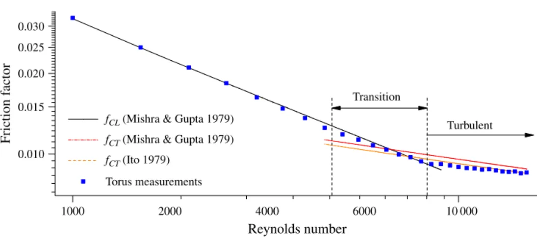
Figure21shows the Fanning friction factor

f =₂_ρUd ₂_1ϕ1p, (3.3)

determined from pressure-loss measurements (squares). The measurements are in good agreement with published data for helical pipes, particularly for the laminar regime. Deviations from the laminar friction factor fCL approximated by the power law of Mishra & Gupta (1979) become appreciable for Re & 2000, beyond which the measured friction factor decays more rapidly than the power law. This trend is alleviated by the onset of oscillations at Rec1, at which point the slope of the friction factor should change. However, we do not have enough data to resolve the change of the slope unambiguously. After a transitional range a further change of the slope of f _{can be clearly recognized at Re ≈ 8000. For Re & 8000 the measured data are in} reasonably good agreement with the correlation fCT of Ito (1959) for helical pipes.

4. Discussion

The torus experiment revealed an initial instability of the toroidal-pipe flow in the bulk to a travelling wave at Re = 4075. As the Reynolds number is increased from its critical value the amplitude of the fundamental Fourier mode grows continuously and

, on

30 May 2017 at 21:24:59

.

(25)

homogeneously, indicating a forward Hopf bifurcation. For Re & 4400 the fundamental frequency develops sidebands. We anticipate that the sidebands are caused by an incommensurate frequency. The travelling wave represents a large-scale structure occupying the full cross-section of the pipe. In addition, we find intermittent small-scale and nearly streamwise vortices which are localized in the wall layer in the vicinity of the impingement point C. For Re & 8000 the spectrum becomes broadband and the signal exhibits high-frequency fluctuations. The corresponding threshold Reynolds number bracketed by PIV was confirmed by pressure-drop measurements which revealed a continuous dependence of the pressure drop on Re with a sudden reduction of the slope at Re ≈ 8000.

Since flow instabilities in toroidal pipes have only been considered by Piazza & Ciofalo (2011), albeit for periodic boundary conditions, our results can only be further compared with the results for helical pipes of Sreenivasan & Strykowski (1983) and Webster & Humphrey (1993, 1997). Regarding the friction factor measurements in the transitional regime, we compare our results with those of Cioncolini & Santini (2006) for helical pipes. When comparing with helically coiled pipes it is tacitly assumed that the particular driving mechanism in the present experiment does not significantly modify the bulk flow, nor does the small pitch of the helical winding (see e.g. Berger et al. 1983; Piazza & Ciofalo 2011). Common to all these investigations, the loss of stability of the steady basic flow occurs in the range 4000 6 Rec16 6000 with a subsequent travelling wave regime for Re> Rec1.

Sreenivasan & Strykowski (1983) used a curvature ratio of _{δ = 17.2}−1 _{= 0.058} which is similar to the present value of _{δ = 0.049. Our quantitative results are in} good agreement with their qualitative observations. Sreenivasan & Strykowski (1983) detected periodic and quasi-periodic low-frequency oscillations near the inner wall of the pipe and high-frequency bursts near its outer wall. The signals were detected by two hot-wire probes in the midplane and at 0_{.125 d from the wall at points A and} C. The slightly larger critical Reynolds number of Re = 4200 obtained by Sreenivasan & Strykowski (1983) may be due to the small difference in δ and/or the small amplitude of the travelling wave at the loci of the hot-wire probes (cf. figure 14). Furthermore, the low-frequency signals measured by Sreenivasan & Strykowski (1983) at Re = 5000 have neither a constant amplitude nor a constant frequency. In fact, they are very similar to our result for the quasi-periodic regime (see e.g. P5 in figure 20). Also, the coexistence of a low-frequency modulated wave with short, high-frequency bursts in different regions of the flow for Re = 5870 is consistent with the present findings. As Sreenivasan & Strykowski (1983) did not specify any wavelengths or amplitudes, a more quantitative comparison cannot be made.

Webster & Humphrey (1993) investigated a nominally fully developed flow through a helically coiled pipe with a curvature ratio of _{δ = 18.2}−1 _{= 0.055 using LDV. The} curvature ratio is even closer to the present value. In the range 5060 6 Re 6 6330 the authors found periodic flow oscillations with a constant fundamental Strouhal number ˆf = 0.25 measured in the inner half of the pipe cross-section. This is qualitatively compatible with our result. However, we find a nearly linear variation of the fundamental frequency from ˆf_{(Re = 5060) = 0.32 to ˆf(Re = 6330) = 0.15.}

When comparing with the above investigations it must be noted that Sreenivasan & Strykowski (1983) used a long straight-pipe section before the inlet of the coiled pipe, whereas Webster & Humphrey (1993) used a ‘flow straightener’ in the straight-pipe section, about thirty pipe diameters upstream of the inlet of the curved pipe. For Reynolds numbers at which the flow is turbulent in the straight pipe two experiments

, on

30 May 2017 at 21:24:59

.

(26)

may represent quite different inlet conditions for the curved pipe. This could be the reason why the first critical Reynolds number Rec1= 5060 determined by Webster & Humphrey (1993) is well above the critical Reynolds number determined by Sreenivasan & Strykowski (1983), and also larger than the present critical Reynolds number Rec1= 4075.

The numerical simulations of Webster & Humphrey (1997) revealed that the amplitude of the travelling wave is very small near the midplane and that the maximum streamwise velocity perturbations arise in the centre of region I. This is confirmed by our measurements (compare figure 7 of Webster & Humphrey 1997

with figures 12 and 14). Wavelengths and phase velocities are of the same order of magnitude, even though differences remain.

The only study to date of the transition to turbulence in a torus is due to Piazza & Ciofalo (2011). For curvature ratios _{δ = 0.1 and δ = 0.3 they numerically simulated} the flow in a torus, driven by an artificial azimuthal body force, for periodic boundary conditions and several Reynolds numbers in the range from 3500 to 14 700. Upon an increase of the Reynolds number Piazza & Ciofalo (2011) found stationary, periodic, quasi-periodic and chaotic flows. The flow states found are in qualitative agreement with our experimental results. However, there are differences.

For _{δ = 0.3, a value much larger than the present curvature ratio δ = 0.049, Piazza} & Ciofalo (2011) reported a supercritical Hopf bifurcation at Rec= 4575, giving rise to a travelling wave along the Dean vortices. A second Hopf bifurcation between 5042_{< Re < 5270 led to a quasi-periodic flow where the additional frequency is} associated with oblique vortices located near the outer equator at C. While the sequence of bifurcations and the regions where the two waves have a sizable amplitude agree qualitatively with our results, the symmetry with respect to the midplane differs, because both modes found by Piazza & Ciofalo (2011) are anti-symmetric with respect to the equatorial plane.

For _{δ = 0.1, a value much closer but yet a factor of two larger than the present} curvature ratio, the periodic and quasi-periodic waves found by Piazza & Ciofalo (2011) are mirror-symmetric as in our measurements, but the first instability at Rec= 5175 is a saddle-node bifurcation associated with a subcritical Hopf bifurcation. In contrast, we find a supercritical Hopf bifurcation for _{δ = 0.049. This difference} might be attributed to the different curvature ratios investigated. It is also not precluded that the different boundary conditions lead to different finite amplitude flow patterns when different modes of the corresponding linear-stability problem are only weakly damped.

Piazza & Ciofalo (2011) have sketched a tentative map of flow states in the_(δ, Re)-plane (their figure 30). Accordingly, the range of chaotic flow is strongly stabilized as δ is increased from zero, giving way to symmetry-breaking bifurcations at larger δ. In order to elaborate their flow map, further experimental investigations for smaller δ would be desirable.

Despite the differences in the setup and the boundary conditions of the above studies on curved pipe flow, there exists no sharp jump in the friction factor upon transition to turbulence as is known from the flow in straight pipes. In the present toroidal pipe flow the flow changes gradually and the friction factor is a monotone function of Re. Thus no distinct onset of turbulence can be detected by pressure drop measurements. However, we found indications for an onset of chaotic motion at Rec2≈ 4400 and a clear change of the slope of f in the logarithmic friction factor diagram at Re ≈ 8000 which we could correlate, by PIV measurements, to the onset of irregular high-frequency fluctuations.

, on

30 May 2017 at 21:24:59

.