THREE METHODS TO CALCULATE THE PROBABILITY OF RUIN BY FRANCOIS DUFRESNE AND HANS U. GERBER
University of Lausanne, Switzerland
ABSTRACT
The first method, essentially due to GOOVAERTS and DE VYLDER, uses the connection between the probability of ruin and the maximal aggregate loss ran-dom variable, and the fact that the latter has a compound geometric distribu-tion. For the second method, the claim amount distribution is supposed to be a combination of exponential or translated exponential distributions. Then the probability of ruin can be calculated in a transparent fashion; the main problem is to determine the nontrivial roots of the equation that defines the adjustment coefficient. For the third method one observes that the probability, of ruin is related to the stationary distribution of a certain associated process. Thus it can be determined by a single simulation of the latter. For the second and third methods the assumption of only proper (positive) claims is not needed.
KEYWORDS
Probability of ruin; discretization; combination of exponentials; simulation. 1. INTRODUCTION
Traditionally, practitioners have approximated the probability of ruin by the expression e~Ru, where R is the adjustment coefficient (by some authors called
insolvency coefficient or Lundberg's constant) and u the initial surplus. From a technical point of view, the need for such an approximation has become less important; thanks to the arrival of efficient computers and even personal com-puters, the exact probability of ruin can be calculated. This has been demons-trated by several authors, i.a. THORIN and WIKSTAD (1976), SHIU (1988), MEYERS and BEEKMAN (1987), PANJER (1986), and indirectly by STRG-TER (1985).
In this paper we shall present three methods; they have the merit that they can be explained in elementary terms and they can be implemented numerically without any difficulty.
The method of upper and lower bounds (section 2) is a method of numerical analysis and is essentiallly due to GOOVAERTS and DE VYLDER (1984). The main drawback of this method is that it is limited to the situation where negative claims are excluded.
Method 2 (section 3) is analytical in nature (but it can be understood without extensive knowledge of complex analysis); it generalizes a method that has been proposed by BOHMAN (1971). If the claim amount distribution is a combination
of exponential or translated exponential distributions, the probability of ruin will be of the form as shown in formula (42). The main task is the numerical determination of the nontrivial (possibly) complex roots of the equation that defines the adjustment coefficient.
The probability of ultimate ruin can also be obtained by simulation (sec-tion 4), although this seems to be a paradoxical idea at first sight. If the claims are reinsured by (for example) an excess of loss contract, the distribution of retained claims cannot by approximated by a combination of exponential dis-tributions, and Method 2 cannot be applied. Method 3 is generally applicable and does not have the drawbacks of Method 1 (no negative claims) or Method 2 (no reinsurance).
2 . METHOD OF UPPER AND LOWER BOUNDS
2.1. Introduction
In this section we shall present a method that leads to the bounds that are due to
GOOVAERTS and DE VYLDER (1984); our derivation will be very similar to PAN-JER'S presentation (1986) and along the ideas of TAYLOR (1985).
2.2. The Model
In the following we shall use the model and the notation of continuous time ruin theory as it is explained in the text by BOWERS et al. (1986, sections 12.2, 12.5,
12.6). Thus
(1) U(t) = u + ct-S(t)
is the insurer's surplus at time t > 0. Here u > 0 is the initial surplus, c the rate at which the premiums are received, and S{t) the aggregate claims between 0 and t. It is assumed that S(t) is a compound Poisson process, given by the Poisson parameter X (claim frequency) and the distribution function P(x) of the indivi-dual claim amounts. In this section we assume that P{0) = 0 (no negative "claims"); afterwards this assumption will be dropped.
The mean claim size is denoted by px. Of course we assume that c exceeds
kpx, the expected payment per unit time. The relative security loading 6 is
defined by the condition that c = (1 + 6)Xpx.
We denote by y/(u) the probability of "ruin", i.e. that U(t) is negative for some t> 0. It is well known that y{0) = 1/(1 + 0). For notational convenience we denote this quantity by q.
The maximal aggregate loss,
(2) L= max iS(/)-ct},
THREE METHODS TO CALCULATE THE PROBABILITY OF RUIN 7 3
is a random variable of great interest, since
(3) 1 - y/(u) = Pr (L<u), u>0,
i.e. the probability of survival is the distribution function of L, see BOWERS et al. [1986, formula (12.6.2.)]. We can write L as a random sum,
(4) L = Ly+L2+ ... +LN,
see BOWERS et al. [1986, formula (12.6.5)]. Here TV is the number of record highs of the process S(t) — ct and has a geometric distribution:
(5) Pr(N=n) = (l-q)qn, n = 0 , 1 , 2 , . . . . The common distribution function of the L,'s is
(6) H(x) = — \ [l-P(y)]dy. Pi J o
Furthermore, the random variables N,Ll,L2,... are independent.
Thus L has a compound geometric distribution,
oo
(7) Pr(L<u)= 2 (l-q)q"H*"(u).
Together with (3) this yields the convolution formula for the probability of ruin, which is often attributed to BEEKMAN (1974, section 13.4), but can also be found in DUBOURDIEU (1952, p. 246).
2.3. Derivation of the bounds
Since H(x) is a continuous distribution function, the expression of the right hand side of (7) cannot be evaluated directly. According to PANJER (1986), the idea is to replace H(x) by one or several discrete distributions. Here we prefer to go one step back and use (4) as a starting point.
For the ease of presentation and notation we assume that the interval of dis-cretisation is the unit interval (in fact this means that the monetary unit is identical to the length of the interval of discretisation). Then we introduce two new random variables that are closely related to L:
(8) L/
and
(9) L" = [L,
Thus the idea is to round the summands in (4) to the next lower integer, which gives (8), or to the next higher integer, which gives (9). Clearly
(10) L'<L<LU,
(11) PT(L'>U)<PT(L>U)<PT(LU>U)
for all u. Since y/(u) = Pr(L > u) is a continuous function for u > 0, it follows that
(12) Pr(L< >u)<y/(u)<Pr(Lu>u), u>0.
Since the distributions of L1 and L" can be calculated recursively, these bounds are of a practical interest.
2.4. Numerical evaluation of the bounds
Let hlk denote the probability that a given summand in (8) is equal to k, i.e., that a given summand in (4) is between k and k+l. Thus
(13) h'k = H(k+l)-H(k), k = 0 , 1 , 2 , . . . .
Let h\ denote the corresponding probability for the summands in (9). Thus (14) h\ = H{k)-H(k-\), A: = 1 , 2 , 3 , . . . .
Here H{x) is given by formula (6). We want to calculate (15) tf=Pr(L' = i), i = 0 , 1 , 2 , . . . and (16) fiu = Pr(L" = i), i = 0 , 1 , 2 , . . . . Then d 7 ) i - 2 / ^ y ( w ) ^ i - 2 • / ; • " > " = o , i , . . . , i = 0 1 = 0 according to (12).
The probabilities (15) and (16) can be calculated recursively by the formu-las n«\ f>- l q (18) Jo -l
(19) y;.'
=_ « 2 / , '
ty / _
t, / = i ,
2 >. . .
l-qh'o k=\ and (20) fou=i-g, i/;" = 4 ] >
A " * / /1- * ,/ = i , 2 , . . . .
it=iTHREE METHODS TO CALCULATE THE PROBABILITY OF RUIN
(22) Pr(L' = i) = Pr(L' = /1 N = 0) • Pr(yV = 0)
75
= i N>\, [Lr] = k)-Pr(N> 1, [Lr] = k)
k=0
for / = 0, 1,2,.... Thus for i = 0 (23) /o' = 1 -which gives (18), and for / = 1, 2 , . . . (24) f!=Ql
which yields (19). For the derivation of (20) and (21) we simply replace the superscript " / " by " « " and observe that h"0 = 0.
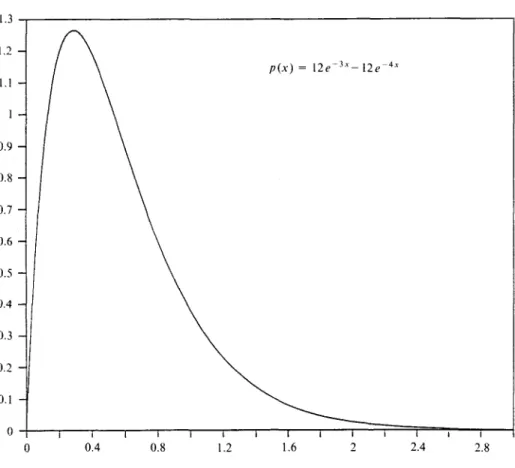
FIGURE 1. Combination of exponential densities.
TABLE 1
UPPER AND LOWER BOUNDS FOR THE PROBABILITY OF RUIN
u .0 .5 1.0 1.5 2.0 2.5 3.0 3.5 4.0 4.5 5.0 5.5 6.0 6.5 7.0 7.5 8.0 8.5 9.0 9.5 10.0
1
.583333 .373585 .226752 .136653 .082274 .049528 .029814 .017947 .010804 .006504 .003915 .002357 .001419 .000854 .000514 .000309 .000186 .000112 .000068 .000041 .000024 lower bounds .583333 .374626 .228198 .138040 .083424 .050410 .030461 .018406 .011122 .006720 .004061 .002454 .001483 .000896 .000541 .000327 .000198 .000119 .000072 .000044 .000026 .583333 .375144 .228921 .138736 .084002 .050855 .030788 .018639 .011284 .006831 .004135 .002504 .001516 .000918 .000555 .000336 .000204 .000123 .000075 .000045 .000027l_
1 1
.583333 .376177 .230367 .140132 .085165 .051753 .031449 .019110 .011613 .007057 .004288 .002606 .001583 .000962 .000585 .000355 .000216 .000131 .000080 .000048 .000029 .005 1 n 1 .02 upper bounds .583333 .376692 .231089 .140831 .085750 .052206 .031783 .019350 .011780 .007172 .004366 .002658 .001618 .000985 .000600 .000365 .000222 .000135 .000082 .000050 .000031 .583333 .377718 .232535 .142234 .086926 .053119 .032459 .019835 .012120 .007406 .004526 .002766 .001690 .001033 .000631 .000386 .000236 .000144 .000088 .000054 .000033length of interval of discretisation
REMARK: In order to keep the paper self-contained, we gave an elementary proof of the recursive formules (19) and (21). They could also have been obtai-ned from the observation that the compound geometric distribution is a special case of the family of the compound distributions considered by PANJER (1981). For the reader who is familiar with renewal theory formulas (19) and (21) are easy to understand. The solution of such a renewal equation is a compound geometric distribution. Thus in this particular context we use this relationship backwards, i.e., that a discrete compound geometric distribution can be inter-preted as the solution of a renewal equation.
2.5. Illustration
For a numerical illustration we assume a claim amount distribution with a pro-bability density function
(25) p(x) = I2(e-ix-e-4x), x>0,
which is shown in figure 1. Written as
it can be interpreted as a combination of exponential densities, where the coef-ficients are 4 and - 3 . The mean claim size is
,27, , , . 4 1 - 3 1 . 1 .
We assume further that X = c = 1; thus 0 = 5/7. From (26) we get
(28) P(x) = \-4e~3x+3e-4x, x>0.
Using (6) we obtain
(29) H{x)=\ e~3x + -e~4x, x>0.
The method of upper and lower bounds has been used for discretisation inter-vals with length .02, .01 and .005. The resulting bounds are displayed in table 1. (The first line, u = 0, shows the known exact value, q — 1/(1 + 0) = 7/12).
3 . COMBINATIONS OF EXPONENTIAL DISTRIBUTIONS AND THEIR TRANSLATIONS
3.1. Improper claims
In section 2 negative claims were excluded, P{0) = 0. If the claims can be nega-tive, 0 < P(0) < 1, the method of section 2 cannot be applied. (The basic formu-las (3) and (4) still hold; but the parameter q of the geometric distribution of N is unknown, as well as the common distribution of the L,'s). We shall present two methods for this more general situation. The first is for a particular family of claim amount distributions; the second will be dicussed in section 4.
3.2. A special family of claim amount distributions
We assume that the claim amount distribution is either a combination of expo-nentials, with probability density function of the form
n
(30) p(x)= ^ Aifiie-"", x>0,
/=i
or else a distribution that is obtained if a combination of exponentials is trans-lated by T > 0 to the left; then the probability density function is
(31) />(*)= 2 4-Ae-
AU+T)> x>-z.
i=i
The /J,'s are positive parameters; for simplicity we assume 0 < fi\ < fi2 < • • • < Pn •
(32) Al+A2+ ...+An=\.
If all the Aj's are positive, (30) is a mixture of exponential densities, and (31) is a translation of a mixture of exponential densities.
The family of combinations of exponentials is much richer (and therefore more useful) than the family of mixtures; note that for the latter the mode is necessarily at 0. In the following we shall treat (30) as a special case (T — 0) of (31). We shall show how the probability of ruin can be calculated, if the claim amount distribution has such a density.
3.3. A functional equation
By distinguishing according to time (say /) and amount (say x) of the first claim we see that the probability of ruin satisfies the following functional equation:
\
JO
(33) y/(u) = \ Xe~h\ y/(u + ct-x)dP(x)dt
O J
r
Jo
Jo
In a sense, this equation has a unique solution:
LEMMA: The functional equation
(34) g(u) = \ Xe~/•oo _ ^ ru+ctu \ g(u + ct—x) dP(x) dt
Jo J - T
f
Jo
' 0
has exactly one solution g(u), u>0, with the property that g(oo) = 0.
PROOF: Since t//(u) is a solution, such a solution exists. To show the uniqueness,
we assume that there are two different solutions g\(u) and g2(u) with
g{(oo) = g2(oo) = 0. Then their difference S(u) = gl(u)-g2(u) satisfies the
equation
= J
(35) S(u)=\ Xe'h\ S(u + ct-x)dP(x)dt.
Now let m = max I 8{u) I and let v be a point at which the maximum is
H>0
THREE METHODS TO CALCULATE THE PROBABILITY OF RUIN 7 9 (36) m = I 6(v) I < m I Xe~poo fv + ctXl \ dP(x) dt Jo J - i Too = m l Ae~A'P
Jo
which is impossible. Thus it is not possible that there are two different solutions that vanish at oo. Q.E.D.
The lemma provides us with a simple tool to determine the probability of ruin. If we can construct a function g{u) that satisfies (34) and vanishes at oo, we know that it is the function \//{u).
3.4. Construction of a solution
We try to solve (34) by an expression of the form
n
(37) g(u)= 2 C
ke~
rtU, u > 0 .
k=\
We substitute this and (31) into (34). After some calculations we obtain the condition that
i n n A R C 1
(38) 2 C
ke-**X 2
1=1 k=\ (Pi-rk)(X+rkc)
Comparison of the coefficients of Cke'rk" yields the condition that
(39) 1 =
But this means that r{,r2,..., rn must be roots of the equation
(40) A+cr = A 5 Ai——e-",
i=i 0?,—0
which is the equation that defines the adjustment coefficient.
XA-Now we compare the coefficients of !_£-&(«+*) in (38). This gives
(41) 2 — Q
= 1-*=i Pt-rk
Our preliminary result is the following: if ry, r2,..., rn are solutions of (40), and
if Q , C2,..., Cn satisfy (41) for / = 1, 2 , . . . , n, expression (37) is a solution of
(34). But how can we be sure that g(oo) = 0?
3.5. The probability of ruin
The function (37) vanishes at oo, if all the rks are positive or (if some are
complex) have a positive real part. Thus the question arises, if equation (40) has n such solutions. Two cases have to be distinguished.
1) If all the Aj's are positive (i.e. the claim amount distribution is a mixture or a translated mixture of exponentials) the answer is easy to obtain. The geome-tric argument of BOWERS et al. (1986, figure 12.7) can also be applied if x > 0. Thus in this case equation (40) has n positive solutions r{, r2,..., rn with
O o " ! = R</]l<r2</]2<...<rn<Pn.
2) If some of the ,4,'s are negative, the situation is more complicated, since some of the solutions of (40) may be complex. But even here one can show that equation (40) has exactly n solutions that are positive or have a positive real part; the interested reader is refered to DUFRESNE and GERBER (1988, Appendix). It is possible that some of the rk% coincide; in the following we
exclude this unlikely situation from our discussion.
Thus we have found the following result: The probability of ruin is
n
(42) .
W{u)= 2 Q«r
r*";
A r = lhere rx, r2, ...,rn are the n roots of equation (40) that are positive or have a
positive real part, and the coefficients C\,C2, ...,Cn are the solutions of the
system of linear equations
(43) 2 - ^ Q = 1, i = 1,2,...,n. *=i P—rk
(Such a system has a unique solution, which we shall determine in the following paragraph).
REMARK: CRAMER (1955, section 5.14) derived (42) for the case 1) above; howe-ver he did not give any explicit formulas for the Q's.
THREE METHODS TO CALCULATE THE PROBABILITY OF RUIN 8 1
3.6. The coefficients
To determine the coefficients we consider the rational function
n i n n / o
2
- n
^-rd n —
(44) Q(x)= ^ "V Pj
n (*-
rk)
k=\
We note that Qifij) = \/Pj,j— 1, 2 , . . . , « . By the principle of partial fractions there are unique coefficients D\,D2,..., Dn such that
(45)
2—^
= Q(x).k=\ x-rk
They can be determined by the condition that the expression on the two sides must be equal for n different values of x, for example for x = Pj U= 1,2,..., n):
(46) 2 -^- \
But this system is equivalent to (43), and we find as a first result that
(47) Ck = Dk, k= 1 , 2 , . . . , « .
Finally we determine these coefficients as follows. First we multiply (45) by
(x-r,,) to get
n j n
(48)
fc=i x—ru "
n (^-»
For x = rh this gives
« . «
(49) Dh=—^^
\ \ flj-fij
k=l k*h
REMARK: The case where c = 0 is of some unexpected interest: Then t//(u) can
be interpreted as the probability of ruin in a discrete time model in which the annual premium is T and the probability density function of the annual aggregate claims is given by (30).
3.7. The case x = 0
In the special case where the claim amount distribution is a combination of exponentials (without translation), there is an alternative and somewhat simpler expression for the coefficients.
First of all, there is an alternative way to get the rks. We replace A
by 1 + - ^
in (40), substract X on both sides, and divide the resulting equation by r to get the condition that
(50) c = X% . Then /"[, r2, • • •, rn are the roots of this equation.
Now consider the rational function
1
(51) Q(x) = B,-x
/=!
fii-where ^! = ^ -^//A- Since Q(x) has the same poles as Q{x) and since
we conclude that Q{x) is in fact identical to the function
Q{x). Thus we gather from (45) that
(52) 2 -^- = Q(x).
k=\ x-rk
THREE METHODS TO CALCULATE THE PROBABILITY OF RUIN 8 3
« A
(53,
*=i x-rk
<•=! A —
Now we let x-* rh. The the denominator of the expression on the right will tend
to the derivative of the function n J
1 V A>
X
Z
ci=l P~X
at x = rh. Thus in the limit we obtain from (53) the formula
(54) Dh =
2
'=1 \Pi-rh)
which (if T = 0) can be used instead of (49).
REMARK : A formula that is essentially identical to (54) has been given by BOH-MAN (1971) for the case of mixtures of exponentials. A result similar to (54) can be found in CRAMER (1955, section 5.14), see also SHIU (1984). The importance of combinations of exponentials has been recognized by THORIN and WIKS-TAD (1977) and GERBER, GOOVAERTS and KAAS (1987).
3.8. Illustration
We consider two examples:
a. For the first example we use the combination of exponential densities of section 2.5, where T = 0 and
(55) n = 2, A = 3, p2 = 4, AY = 4, A2= -3,
and assume, as before, X = c = 1. The solutions of (50) are r, = 1, r2 = 5.
Then we get from (54) and (47)
Cx = 5/8, C2= - 1/24 .
Thus the probability of ruin is given by the expression = -e-u-— e~5u.
TABLE 2
THE PROBABILITY OF RUIN FOR COMBINATIONS OF EXPONENTIAL DISTRIBUTIONS AND THEIR TRANSLATIONS b . 0 . 1 .0 .5 1.0 1.5 2.0 2.5 3.0 3.5 4.0 4.5 5.0 5.5 6.0 6.5 7.0 7.5 8.0 8.5 9.0 9.5 0.0 0.583333 .375661 .229644 .139433 .084583 .051303 .031117 .018873 .011447 .006943 .004211 .002554 .001549 .000940 .000570 .000346 .000210 .000127 .000077 .000047 .000028 0.584204 .365203 .219122 .130687 .077873 .046396 .027642 .016468 .009812 .005845 .003483 .002075 .001236 .000736 .000439 .000261 .000156 .000093 .000055 .000033 .000020
The numerical values are shown in table 2, column a., and confirm our findings of table 1.
b. For the second example we translate the probability density (26) by 0.1 to
the left. Thus the claim amount distribution is now given by x — 0.1 and (55). The mean size is now
px = 7/12-0.1 = 29/60.
We assume the same relative security loading as in the first example, 0 = 5/7. Thus, if for example c = 1, we assume k = 35/29. From (40) we find
rx = 1.035774, r2 = 4.817225.
From (49) and (47) we obtain
C, = 0.618102, C2 = -0.033898 .
Then the probability of ruin is given by the expression
THREE METHODS TO CALCULATE THE PROBABILITY OF RUIN 8 5
4 . SIMULATION
4.1. Introduction
If the probability of a certain event is to be found by simulation, the usual proceeding is to repeat the stochastic experiment a number of times and to see each time, if the event does or does not take place. Then the observed empirical frequency is used to estimate the probability of the event.
Obviously, this method of brute force is not very pratical, if we are to find the probability of ultimate ruin. Nevertheless the probability of ultimate ruin can be obtained by simulation, if the following two facts are kept in mind: Firstly, the probability of ruin is equivalent to the stationary distribution of a certain asso-ciated process, and secondly, this stationary distribution can be obtained by pathwise simulation.
4.2. Duality Let us introduce
(56) L(t) = S(t)-ct, t>0, the aggregate loss at time t, and
(57) M(t) = m a x L(z), t>0,
0<z</
the maximal aggregate loss in the interval from 0 to t. Then (58) \
i.e., the probability of survival to time t (a function of the initial surplus) is the distribution function of M{t). Note that (58) generalizes (3).
We shall also consider
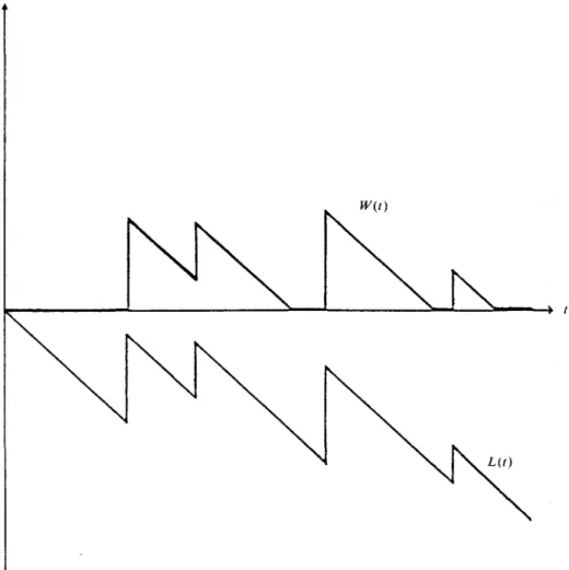
(59) W(t) = L(t)- min L(z). 0<z<l
The process { W(t)\ is obtained from the process [L{t)\ by introduction of a retaining barrier at 0. This is illustrated in figure 2.
Let
(60) F(x, t) = Pr(W(t)<x)
denote the distribution function of W(t). Now we rewrite (59) as follows (61) W{t) = max [L(t)-L(z)\.
FIGURE 2. Construction of the process j W(t)\.
W(t)
L(t)
Since the process \L(t)} has stationary and independent increments, it follows that W{t) and M(t) have the same distribution. Therefore
(62)
Let
(63)
\-y(u,t) =
F(x) = lim F(x, t)
denote the stationary distribution of the process j W{t)\. Then it follows from (62) that
THREE METHODS TO CALCULATE THE PROBABILITY OF RUIN 8 7
(64) \-W{U) = F{u).
It remains to show how F(u) can be obtained efficiently.
REMARKS: The fact that W(t) and M(t) are identically distributed is well known, see for example FELLER (1966, VI.9) or SEAL (1972).
4.3. Determination of the stationary distribution
The distribution F(x) can be obtained by pathwise simulation in the following fashion: For a particular value of x let D(x, t) denote the total duration of time that the process { W(z) \ is below the level x before time /. Then one can show that
(65) -> F(x) for t -> oo. t
This is essentially an application of the Strong Law of Large Numbers and can be found in HOEL, PORT and STONE (1972, section 2.3). From (64) and (65) we see that the probability of ruin can indeed be obtained by simulation, where the process { W(t)) has to be simulated only once.
4.4. Practical implementation
We simulate Tx, T2,..., the times when the claims occur, and XY,X2,..., the
corresponding claim amounts. Instead of keeping track of D(x, t), it is easier to keep track of Dn(x), the duration of the time that the process { W(t)\ is below
the level x before the time of the n-th claim. Then it follows from (65) and the fact that Tn -> oo for n -» oo that
n
(66) > F(x) for n -» oo.
Thus if n is sufficiently large, l-i//(u) = F(u) is estimated by the value of Dn(u)/Tn.
For a given value of x, Dn (x) can be computed recursively as follows. First
Di(x) = T{. Then for n = 1,2,...
(67) if Wn+Xn<x
w
" • if Wn + XH>x.
Here Wn denotes the value of W(t) immediately before the «-th claim. Thus
(Wn + Xn)+ is the value of W(t) just after the «-th claim. Therefore we can
calculate the W^s recursively according to the formula (68) = [(Wn + Xn)+-c(Tn+l-Tn)]+ ,
with starting value Wx = 0.
4.5. Illustration
We condider the two examples of section 3.8. Each time the simulation has been carried out through 1 million claims, and the results are shown in table 3a and table 3b. We note that in each column the estimators for the probability of ruin approach the exact value (taken from table 2) as simulation progresses. We note that the convergence is quite satisfactory, perhaps with the exception of the "large" values of u, where the probability of ruin is small. In any case, if one is not satisfied with the convergence, the simulation can be continued to obtain more precise results. Of course for this it would be advisable to do the simula-tion on a mainframe computer! (The simulasimula-tions above have been carried out on a PC).
u = 0
TABLE 3a
PROBABILITY OF RUIN BY SIMULATION
2 3 4 n 500 100000 150000 200000 250000 300000 350000 400000 450000 500000 550000 600000 650000 700000 750000 800000 850000 900000 950000 1000000 exact 0.588746 0.581629 0.581775 0.582200 0.583733 0.583160 0.582982 0.582879 0.582922 0.583052 0.583466 0.583861 0.583791 0.583743 0.583600 0.583540 0.583609 0.583758 0.583820 0.583951 0.583333 0.254429 0.221634 0.222313 0.223009 0.224995 0.224523 0.224037 0.223622 0.223279 0.223807 0.224405 0.224748 0.224570 0.224869 0.224708 0.224802 0.224789 0.225065 0.225186 0.225311 0.229644 0.127094 0.077008 0.077642 0.078331 0.079864 0.079211 0.079002 0.078979 0.078748 0.079288 0.079577 0.079699 0.079593 0.079917 0.079819 0.079999 0.079971 0.080087 0.080183 0.080232 0.084583 0.076168 0.027749 0.027530 0.027859 0.028884 0.028330 0.028149 0.028174 0.028017 0.028304 0.028410 0.028368 0.028316 0.028544 0.028493 0.028697 0.028726 0.028787 0.028808 0.028808 0.031117 0.028443 0.009953 0.009794 0.009804 0.010299 0.009968 0.009757 0.009790 0.009683 0.009855 0.010002 0.009971 0.009929 O.O1OO73 0.010052 0.010231 0.010262 0.010314 0.010274 0.010221 0.011447 0.011798 0.003666 0.003529 O.OO35O9 0.003720 0.003550 O.OO34O3 0.003423 0.003379 0.003432 0.003567 0.003535 0.003488 O.OO355O 0.003563 0.003646 0.003675 0.003707 0.003668 0.003613 0.004211 0.002875 0.001398 0.001290 0.001262 0.001387 0.001305 0.001233 0.001225 0.001186 0.001200 0.001309 0.001293 0.001261 0.001261 0.001284 0.001303 0.001334 0.001349 0.001321 0.001301 0.001549 0.000U9 O.OOO596 0.000486 0.000454 0.000503 0.000468 0.000450 O.OOO443 O.OOO421 0.000429 0.000494 0.000479 0.000457 0.000445 0.000465 0.000460 0.000436 0.000438 0.000481 O.OOO473 0.000570
THREE METHODS TO CALCULATE THE PROBABILITY OF RUIN 89 TABLE 3b
PROBABILITY OF RUIN BY SIMULATION
n 500 100000 150000 200000 250000 300000 350000 400000 450000 500000 550000 600000 650000 700000 750000 800000 850000 900000 950000 1000000 exact 0.593045 0.584593 0.583346 0.582293 0.582775 0.583533 0.584417 0.584564 0.584437 0.584456 0.584328 0.584500 0.584395 0.584397 0.584731 0.584664 0.584454 0.584524 0.584671 0.584531 0.584204 0.243940 0.214373 0.212020 0.211215 0.212572 0.213759 0.214489 0.214564 0.214486 0.214311 0.213919 0.214244 0.214239 0.214095 0.214306 0.214142 0.213887 0.213940 0.214196 0.214211 0.219122 0.091826 0.074654 0.072741 0.072141 0.073010 0.073920 0.074245 0.074286 0.074457 0.074225 0.073795 0.074049 0.074237 0.074108 0.074305 0.074188 0.074059 O.O74OO2 0.074177 0.074280 0.077873 0.034948 0.027335 0.026267 0.025765 0.026148 0.026537 0.026771 0.026818 0.027060 0.026841 0.026510 0.026507 0.026734 0.026711 0.026732 0.026633 0.026543 0.026448 0.026499 0.026556 0.027642 0.008195 0.010103 0.009432 0.009309 0.009469 0.009531 0.009687 0.009652 0.009865 0.009749 0.009533 0.009519 0.009640 0.009612 0.009607 0.009533 0.009460 0.009437 0.009438 0.009482 0.009812 0.000000 0.003662 0.003226 0.003361 0.003316 0.003335 0.003398 0.003421 O.OO35O7 0.003449 O.OO335O 0.003382 0.003467 0.003425 0.003393 O.OO334O 0.003308 0.003318 0.003325 0.003337 0.003483 0.000000 0.001404 0.001140 0.001177 0.001122 0.001153 0.001142 0.001131 0.001167 0.001122 0.001072 0.001111 0.001162 0.001144 0.001118 0.001084 0.001068 0.001089 0.001124 0.001123 0.001236 0.000000 0.000710 0.000527 0.000509 0.000453 0.000439 O.OOO4O3 0.000376 O.OOO395 0.000361 O.OOO337 0.000372 0.000393 0.000386 O.OOO373 0.000355 O.OOO353 0.000375 0.000405 0.000400 0.000439 REFERENCES
BEEKMAN, J.A. (1974) Two Stochastic Processes, Almqvist & Wiksell, Stockholm. BOHMAN, H. (1971) "The ruin probability in a special case", ASTIN Bulletin 7, 66-68.
BOWERS, N.L., JR., GERBER, H.U., HICKMAN, J.C., JONES, D. A. and NESBITT, C.J. (1986) Actuarial
Mathematics, Society of Actuaries, Itasca, Illinois.
CRAMER, H. (1955) "Collective Risk Theory — A survey of the theory from the point of view of the theory of stochastic processes", The Jubilee Volume of Skandia.
DUBOURDIEU, J. (1952) Theorie malhematique du risque dans les assurances de repartition, Gauthier-Villars, Paris.
DUFRESNE, F. and GERBER, H. U. (1988) "The Probability and Severity of Ruin for Combinations of Exponential Claim Amount Distributions and their Translations", Insurance: Mathematics &
Economics 7, 75-80.
FELLER, W. (1966) An Introduction to Probability Theory and its Applications, Volume 2, Wiley, New York.
GERBER, H.U., GOOVAERTS, M.J., and KAAS, R. (1987) " O n the Probability and Severity of Ruin",
ASTIN Bulletin, 17, 151-163.
GOOVAERTS, M. J. and DE VYLDER, F. (1984) " A Stable Algorithm for Evaluation of Ultimate Ruin Probabilities", ASTIN Bulletin, 14, 53-59.
HOEL, P. G., PORT, S. C. and STONE, C. J. (1972) Introduction to Stochastic Processes, Boston: Houghton Mifflin.
MEYERS, G., and J.A. BEEKMAN(1988) "An improvement to the convolution method of calculating (</(«)", Insurance: Mathematics and Economics, 6, 267-274.
PANJER, H. H. (1986) " Direct Calculation of Ruin Probabilities", The Journal of Risk and Insurance Vol. 53. Nr. 3, 521-529.
PANJER, H.H. (1981) "Recursive Evaluation of a Family of Compound Distributions", ASTIN
SEAL, H. L. (1972) "Risk Theory and the Single Server Queue", Journal of the Swiss Association of
Actuaries, 171-178.
SHIU, E.S.W. (1984) Discussion of "Practical Applications of the Ruin Function", Transactions of the
Society of Actuaries. 36, 480-486.
SHIU, E.S.W. (1988) "Calculation of the Probability of Eventual Ruin by Beekman's Convolution Series", Insurance: Mathematics and Economics, 7, 41-47.
STROTER, B. (1985) "The Numerical Evaluation of the Aggregate Claim Density Function via Integral Equation", Bulletin of the German Association of Actuaries 17, 1-14.
TAYLOR, G.C. (1985) "A Heuristic Review of Some Ruin Theory Results", ASTIN Bulletin, 15, 73-88.
THORIN, O., and N. WIKSTAD (1976) "Calculation and use of ruin probabilities", Transactions of the
20th International Congress of Actuaries, vol, III, 773-781.
THORIN, O., and N. WIKSTAD (1977) "Calculation of ruin probabilities when the claim distribution is lognormal", ASTIN Bulletin, 9, 231-246.
F. DUFRESNE and H. U. GERBER