HAL Id: lirmm-01794757
https://hal-lirmm.ccsd.cnrs.fr/lirmm-01794757
Submitted on 17 May 2018
HAL is a multi-disciplinary open access
archive for the deposit and dissemination of
sci-entific research documents, whether they are
pub-lished or not. The documents may come from
teaching and research institutions in France or
abroad, or from public or private research centers.
L’archive ouverte pluridisciplinaire HAL, est
destinée au dépôt et à la diffusion de documents
scientifiques de niveau recherche, publiés ou non,
émanant des établissements d’enseignement et de
recherche français ou étrangers, des laboratoires
publics ou privés.
Distributed under a Creative Commons Attribution| 4.0 International License
Pijus Simonaitis, Krister Swenson
To cite this version:
Pijus Simonaitis, Krister Swenson. Finding Local Genome Rearrangements. 17th International
Work-shop on Algorithms in Bioinformatics (WABI 2017), Aug 2017, Boston, United States. pp.24:1–24:13,
�10.4230/LIPIcs.WABI.2017.24�. �lirmm-01794757�
Pijus Simonaitis
1and Krister M. Swenson
21 ENS Lyon, Lyon, France [email protected]
2 LIRMM, CNRS – Université Montpellier, Montpellier, France; and Institut de Biologie Computationnelle (IBC), Montpellier, France [email protected]
Abstract
The Double Cut and Join (DCJ) model of genome rearrangement is well studied due to its math-ematical simplicity and power to account for the many events that transform genome architec-ture. These studies have mostly been devoted to the understanding of minimum length scenarios transforming one genome into another. In this paper we search instead for DCJ rearrangement scenarios that minimize the number of rearrangements whose breakpoints are unlikely due to some biological criteria. We establish a link between this Minimum Local Scenario (MLS) problem and the problem of finding a Maximum Edge-disjoint Cycle Packing (MECP) on an undirected graph. This link leads us to a 3/2-approximation for MLS, as well as an exact integer linear program. From a practical perspective, we briefly report on the applicability of our methods and the potential for computation of distances using a more general DCJ cost function. 1998 ACM Subject Classification G.2.1 Combinatorial Algorithms, G.2.2 Graph Algorithms, J.3 Life and Medical Sciences
Keywords and phrases genome rearrangement, double cut and join, maximum edge-disjoint cycle packing, Hi-C, NP-complete, approximation algorithm
Digital Object Identifier 10.4230/LIPIcs.WABI.2017.24
1
Overview
The problem of sorting genomes by a prescribed set of biologically plausible rearrangements has been a central problem in comparative genomics for roughly a quarter century. The Double Cut and Join (DCJ) model covers a diverse set of these possible rearrangements while being grounded in a very simple mechanism [15, 2]. An important step forward is the development of methodology to find plausible rearrangement scenarios using biological constraints.
We recently introduced a model for weighting DCJs that is suitable for representing certain biological constraints. The model groups breakpoint regions between adjacent genes (or syntenic blocks) into equivalence classes that are likely to participate in a rearrangement [14]. The 3D spacial proximity of breakpoint regions could be used as such, and the data is becoming increasingly available due to an experiment called Hi-C [9, 13]. (The pertinence of this model is discussed in Section 7.) The model colors adjacencies for use with a binary cost function, where a DCJ acting on adjacencies with the same color is of zero cost while those acting on different colors are of cost one. We showed that the problem of finding – out
This work is partially supported by the IBC (Institut de Biologie Computationnelle) (ANR-11-BINF-0002), by the Labex NUMEV flaship project GEM, and by the CNRS project Osez l’Interdisciplinarité.
© Pijus Simonaitis and Krister M. Swenson; licensed under Creative Commons License CC-BY
of all minimum length rearrangement scenarios – a scenario that minimizes the number of costly moves, takes polynomial time [14].
In this paper we disregard the length of the scenario and instead focus solely on the number of costly moves. We show that the Minimum Local Scenario problem is NP-Hard, while admitting a 3/2-approximation. This is done by exploiting a relationship to the Maximum Edge-disjoint Cycle Packing problem, a problem which was first linked to genome rearrangement in a different way by Alberto Caprara (sorting by unsigned reversals is NP-Hard [4]).
In our method, MLS is transformed into an edge elimination problem on a junction
graph, representing the transitions between colors encountered when traversing the connected
components of the adjacency graph. We give an exact formula for the number of costlyy moves based solely on the number of edges and the number of cycles in the MECP of the junction graph. We also propose an exact algorithm for MLS that is exponential in the number of colors and not in the number of genes and discuss an example where this algorithm is computationally feasible. Finally, we show how to bound the number of non-parsimonious moves when using a more general cost function.
The paper is organized as follows. Section 2 introduces basic definitions. In Section 3 our main result, relating MLS to MECP by way of the junction graph, is described in the simplified realm of sets of pairs. In this context, the junction graph is Eulerian. Section 4 extends the results to the general case where the junction graph is not Eulerian. Section 5 presents our algorithmic results. Finally, Section 6 discusses a more general cost function, while Section 7 reports on practical aspects of coloring adjacencies.
2
Genome and DCJ rearrangements
A genome consists of chromosomes that are linear or circular molecules partitioned into uniquely labeled directed genes (or equivalently syntenic blocks of genes) and intergenic regions separating them.
1
2
3
4
The genome depicted above consists of a linear and a circular chromosome each having two genes. Arrows in the picture indicate the head extremities of the genes. We can represent a genome by a set of adjacencies between the gene extremities and such a set for a genome from our example is){1h}, {1t,2t}, {2h}, {3h,4t}, {4h,3t}*. Here 1hdenotes the head extremity
of a gene 1. An adjacency is either an unordered pair of gene extremities that are adjacent on a chromosome, called internal adjacency, or a single gene extremity adjacent to one of the two ends of a linear chromosome, called an external adjacency.
IDefinition 1 (Double Cut and Join). DCJ move acts on one or two adjacencies as follows: 1. {a, b}, {c, d} æ {a, c}, {b, d} or {a, d}, {b, c}
2. {a, b}, {c} æ {a, c}, {b} or {b, c}, {a}
3. {a, b} æ {a}, {b}
We first treat a simplified instance of sets of pairs where all the adjacencies are internal and DCJs can only swap the elements between them in Section 3. Then in Section 4 we show how genomes can be extended to the sets of pairs and use the previously obtained results to solve the Minimum Local Scenario problem.
3
Minimum Local Scenario for sets of pairs
3.1 Cost of a DCJ scenario
Given two sets of pairs:
A=){1, 2}, . . . , {2n ≠ 1, 2n}*, and B=){q1, q2}, . . . , {q2n≠1, q2n}*,
with pairs being unordered and (q1, . . . , q2n) being a permutation of (1, . . . , 2n), our goal
is to transform A into B with a sequence of DCJ moves {a, b}, {c, d} æ {a, c}, {b, d} and {a, b}, {c, d} æ {a, d}, {b, c}.
A coloring of a set of pairs A over a set of colors is a function col : A æ partitioning
Ainto the subsets of different colors. A coloring is used to define the cost of a DCJ move. A
move is local and of zero cost if it acts on the pairs with equal colors and it is non-local and of cost 1 otherwise. The cost of a sequence of DCJ moves, a DCJ scenario, is the sum of the costs of its constituent moves.
A DCJ move A æ AÕtransforming a set of pairs A into AÕ will also transform col into
colÕ, a coloring of AÕ. This means that a DCJ scenario transforming A into B will transform
A’s coloring col into B’s coloring colB. For a pair p œ A we use notation (p, col(p)) of a
colored pair. Four different DCJ moves on colored pairs ({a, b}, x) and ({c, d}, y) are allowed
in our model giving four possible outcomes: ({a, c}, x), ({b, d}, y), or ({a, d}, x), ({b, c}, y), or
({a, c}, y), ({b, d}, x), or ({a, d}, y), ({b, c}, x).
The biological interpretation of this model is that intergenic regions are broken and repaired at their borders with the gene extremities. We discuss the applicability of such a model in Section 7.
In our previous work [14] we have treated the Minimum Local Parsimonious Scenario problem.
IProblem 1 (MLPS). For two sets of pairs A, B and a coloring of A find a minimum cost
scenario among the DCJ scenarios of minimum length transforming A into B.
We have shown that MLPS takes polynomial time, however the real evolutionary scenario might be non-parsimonious. In this paper we study the Minimum Local Scenario problem which asks for such non-parsimonious scenarios.
IProblem 2 (MLS). For two sets of pairs A, B and a coloring of A find a minimum cost
DCJ scenario transforming A into B.
MLS has the following combinatorial interpretation. Pairs of uniquely labeled balls (set of pairs A) are partitioned into the bins (coloring of A). Given a partition T of the balls into pairs (set of pairs B), find a minimum length sequence of ball swaps between the bins (DCJ moves) so that for all pairs {a, b} œ T, a and b end up in the same bin (A is transformed into B).
3.2 Adjacency and junction graphs
The Adjacency graph was introduced in [2] for the study of DCJ rearrangements. We introduce a transformation of the adjacency graph, called a junction graph, that incorporates the information on a coloring.
I Definition 2 (Adjacency graph). For two sets of pairs A and B the adjacency graph
AG(A, B) is defined as a bipartite multi-graph whose vertices are A fi B and for each p œ A
and q œ B there are exactly |p fl q| edges joining these two vertices.
IDefinition 3 (Junction graph). For two sets of pairs A, B and a coloring col of A over
we define a multi-graph J(A, B, col) = ( , E). For every pair {a, b} œ B we add an edge (x, y) to E such that x and y are the colors of the pairs of A adjacent to {a, b} in AG(A, B).
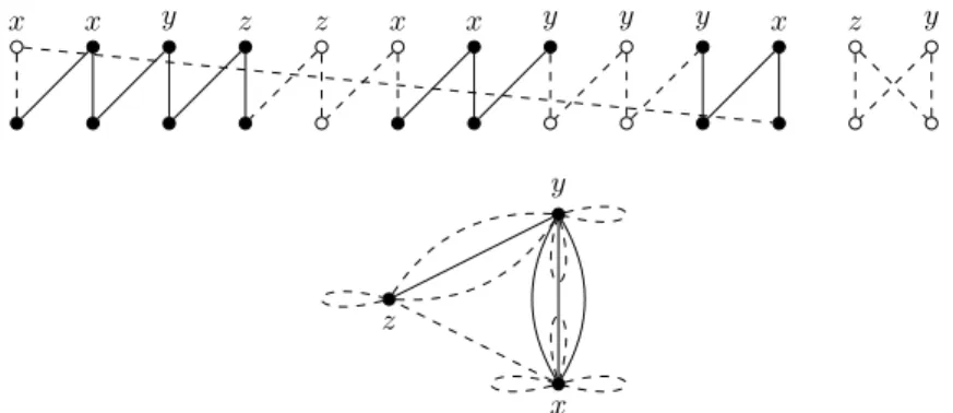
IExample 4. For two sets of pairs A, B and a coloring col of A we present below AG(A, B)
on the left and J(A, B, col) on the right.
A=)({1,2},t),({3,4},x),({5,6},y),({7,8},z),({9,10},x)* B=){2, 3}, {4, 5}, {6, 7}, {8, 1}, {9, 10}* A B t1 2 x3 4 y5 6 z7 8 x9 10 2 3 4 5 6 7 8 1 9 10 t x y z
A DCJ move ({1, 2}, t), ({5, 6}, y) æ ({5, 2}, t), ({1, 6}, y) transforming A into AÕtransforms
adjacency and junction graphs as follows.
AÕ B t5 2 x3 4 y1 6 z7 8 x9 10 2 3 4 5 6 7 8 1 9 10 t x y z
All connected components of AG(B, B) are cycles of length 2 thus at the end of a DCJ scenario transforming A into B we are left with a junction graph whose edges are all loops, we call such a graph terminal.
IDefinition 5 (A DCJ move on a graph). Edges (x, y) and (z, t) of a graph are deleted and
replaced by either (x, z) and (y, t) or (x, t) and (y, z).
ILemma 6. For a DCJ scenario of cost w transforming A into B there exists a DCJ
scenario of length at most w transforming J(A, B, col) into a terminal graph and vice versa.
Proof. From Example 4 it should be clear that for every DCJ move A æ AÕ we have that
a transformation J(A, B, col) to J(AÕ, B, colÕ) is a DCJ move on a graph. If a DCJ move
Aæ AÕ is of zero cost, then J(A, B, col) = J(AÕ, B, colÕ) and such moves will be omitted
from a DCJ scenario on a graph. This means that a DCJ scenario of cost w transforming A (and its coloring col) into (B and its coloring colB) provides us with a DCJ scenario of length
at most w on a graph transforming J(A, B, col) into a terminal graph J(B, B, colB). On
the other hand for every DCJ move on a graph J æ JÕ a DCJ move A æ AÕ can be found
J(A, B, col) into a terminal graph we obtain a DCJ scenario of length w, thus of cost at most w, transforming A and its coloring col into C and its coloring colC such that J(C, B, colC) is
terminal. This means that C’s pairs belonging to the same connected component of AG(C, B) are of the same color. A DCJ scenario transforming C into B and only acting on the pairs belonging to the same connected components of an adjacency graph can be easily found. Such a scenario is of zero cost and at the end we obtain a DCJ scenario transforming A into
Bof cost at most w. J
3.3 Linking DCJ scenarios and Maximum Edge-disjoint Cycle Packings
Using Lemma 6 we can shift our attention from a DCJ scenario on a set of pairs to a DCJ scenario on a junction graph J. From now on we will shorten “DCJ move on a graph” to “DCJ move”.
IDefinition 7 (Maximum disjoint Cycle Packing (MECP)). Maximum
Edge-disjoint Cycle Packing of a graph G is a largest set of edge-Edge-disjoint cycles in G. For a graph G = (V, E) we note E(G) = |E| and c(G) the size of its MECP. For a junction graph J we write w(J) to indicate the minimum length of a DCJ scenario transforming J into a terminal graph.
ITheorem 8. For a junction graph J we have w(J) = E(J) ≠ c(J).
Proof. It is easy to transform a cycle of length n > 1 into n loops in n≠1 DCJ moves. Given a cycle packing C of J we construct a DCJ scenario transforming J into a terminal graph while transforming all of its cycles separately. The length of such a scenario is E(J)≠|C|, and if we take a Maximum Edge-disjoint Cycle Packing we obtain w(J) Æ E(J) ≠ c(J).
Now take a scenario of m DCJ moves transforming J = J0 into a terminal graph Jm,
with Jkbeing the junction graph after k Ø 0 moves of the scenario. We enumerate J’s edges
E= {e1, . . . , eE(J)} and define their partition into singletons P0 = {{1}, . . . , {E(J)}}. A
move k of a scenario acts on two edges ei and ejof Jk≠1, deleting them and introducing
two new edges to give Jk. We call one of these edges ei and another ej, preserving the
enumeration of the edges of Jk. Let Siand Sjbe the subsets of a partition Pk≠1including
eiand ej respectively. We define a partition Pkof {e1, . . . , eE(J)} obtained from Pk≠1by
merging Siand Sjinto Sifi Sj. At the end we obtain a partition P
mof cardinality at least
E(J) ≠ m as there were at most m merges on the way. We will show that Pmis a cycle
packing of J.
For J’s vertices V , a subset S µ {e1, . . . , eE(J)} and k œ {0, . . . , m}, we define SJk = (V, S) a subgraph of Jk. For any graph G and its vertex v we denote dG(v) the degree of v in G.
ILemma 9. For k œ {0, . . . m}, a subset S in a partition Pk, and a vertex v of J we have
dSJ(v) = dSJk(v).
Proof. J0= J, thus the equality is true for k = 0. We suppose that equality is true for every
Sand v with k ≠ 1 and proceed by induction on k. We fix a vertex v and a subset S œ Pk.
The k-th move of a scenario acts on the edges eiand ej that by construction belongs to the
same subset S՜ P
k. There are three possibilities:
1. (SÕ”= S) In this case S œ P
k≠1and SJk = SJk≠1, as the edges in S are unaffected by a
DCJ move. Using the inductive hypothesis we obtain
2. (SÕ= S and S = Sifi Sj with Siand Sj being the different subsets in P
k≠1including ei
and ej respectively) SJk is obtained from SJk≠1 via a DCJ move and, as a DCJ move
does not affect the degrees of the vertices we obtain, we use the inductive hypothesis and the fact that S = Sifi Sj to get
dSJk(v) = dSJk≠1(v) = dSi
Jk≠1(v) + dSjJk≠1(v) = dS i
J(v) + dSJj(v) = dSJ(v) .
3. (SÕ= S and e
i, ejalready present in the same subset S of Pk≠1) SJk is obtained from
SJk≠1 via a DCJ move which does not affect the degrees of the vertices and thus we
obtain (using inductive hypothesis)
dSJk(v) = dSJk≠1(v) = dSJ(v) .
As equality is preserved by a DCJ move and true for k = 0 we obtain the result by
induction. J
All edges of Jmare loops, thus for every subset S in Pmand vertex v of J, dSJm(v) is even and so, using Lemma 9, we know that dSJ(v) is even as well. This means that the connected components of SJ are Eulerian and thus S is a union of J’s cycles. As Pmcontains
at least E(J) ≠ m subsets, we know that it partitions the edges of J into at least E(J) ≠ m cycles. If we take a scenario of length w(J) we obtain the inequality c(J) Ø E(J) ≠ w(J), which ends the proof of Theorem 8. J
4
Minimum Local Scenario for genomes
4.1 Cost of a DCJ scenario
Given two genomes with enumerated extremities
A=){1, 2}, . . . , {2n ≠ 1, 2n}, {2n + 1}, . . . , {2n + 2m}*, B=){q1, q2}, . . . , {q2l≠1, q2l}, {q2l+1}, . . . , {q2n+2m}*,
and (q1, . . . , q2n+2m) being a permutation of (1, . . . , 2n + 2m). Our goal is to transform A
into B using DCJ moves defined in Definition 1. As in the case of pairs-only, we define a coloring col : A æ which is transformed by DCJ moves as follows:
1. ({a, b}, x), ({c, d}, y) æ ({a, c}, x), ({b, d}, y) or ({a, d}, x), ({b, c}, y) or ({a, c}, y), ({b, d}, x) or ({a, d}, y), ({b, c}, x)
2. ({a, b}, x), ({c}, y) æ ({a, c}, x), ({b}, y) or ({a, c}, y), ({b}, x) or ({b, c}, x), ({a}, y) or ({b, c}, y), ({a}, x)
3. ({a, b}, x) æ ({a}, x), ({b}, z) or ({a}, z), ({b}, x) with any color z
4. ({a}, x), ({b}, y) æ ({a, b}, x) or ({a, b}, y)
The cost of a DCJ move is equal to 0 if z = x or x = y, 1 otherwise.
4.2 Genome extensions
A genome can be extended into a set of pairs by adding artificial gene extremities that represent telomeres marking the ends of each linear chromosome.
IDefinition 10 (Genome extensions). For a genome A we define a set A+of the sets of pairs that are genome extensions of A. ˆAœ A+ is of a form:
)
{1, 2}, . . . , {2n ≠ 1, 2n}, {2n + 1, ¶1}, . . . , {2n + 2m, ¶2m}, {¶2m+1,¶2m+2}, . . . , {¶2m+2l≠1,¶2m+2l}*
with l œ N and (¶1, . . . ,¶2m+2l) being a permutation of (2n + 2m + 1, . . . , 2n + 4m + 2l).
A pair {i, j} with i, j > 2n + 2m will be called a telomeric pair. By construction, adjacencies of a genome and non-telomeric pairs of a genome extension can be mapped one to one as internal adjacencies of a genome are present in the genome extension, and external adjacencies are simply complemented by an artificial gene extremity. A coloring col of A can be trivially extended to a coloring ˆcolof ˆAœ A+by keeping the same colors for the non-telomeric
pairs and choosing any colors for the telomeric ones. For every DCJ move A æ AÕacting on
two adjacencies of a genome there is an induced DCJ move ˆAæ ˆAÕof the same cost with ˆAÕœ
AÕ
+acting on the corresponding pairs of a genome extension. For example ({a}, x), ({b}, y) æ
({a, b}, x) induces ({a, ¶1}, x), ({b, ¶2}, y) æ ({a, b}, x), ({¶1,¶2}, y) and ({a, b}, x)({c}, y) æ ({a, c}, x), ({b}, y) induces ({a, b}, x), ({c, ¶1}, y) æ ({a, c}, x), ({b, ¶1}, y). A DCJ move of
the form ({a, b}, x) æ ({a}, x), ({b}, z) or ({a}, z), ({b}, x) acting on a single adjacency is different, as in this case we need a telomeric adjacency of color z to be present in a genome extension. For example ({a, b}, x) æ ({a}, x), ({b}, z) induces ({a, b}, x), ({¶1,¶2}, z) æ ({a, ¶1}, x), ({b, ¶2}, z) on a genome extension including ({¶1,¶2}, z).
ILemma 11. For a DCJ scenario transforming genome A into B and a coloring of A there
exist genome extensions ˆAœ A+, ˆBœ B+ and a scenario of the same cost transforming ˆA
into ˆB.
Proof. In a DCJ scenario there is a certain number l of the DCJ moves acting on a single adjacency. We take a genome extension ˆAœ A+ with l telomeric pairs. Every DCJ move
({a, b}, x) æ ({a}, x), ({b}, z) or ({a}, z), ({b}, x) will induce a move acting on a different telomeric pair of a genome extension and its color will be a color z required by that DCJ move on a genome. In this way every DCJ move on a genome will induce a move on a genome extension and after a scenario of cost w we will end up with ˆB, an extension of genome
B. J
ILemma 12. For a DCJ scenario transforming ˆAœ A+ into ˆBœ B+ and a coloring of A
there exists a DCJ scenario of the same cost or smaller transforming A into B.
Proof. We start with a couple (A, ˆA) and apply a scenario transforming ˆAinto ˆBstep by
step, transforming A on the way. After the first k moves of a scenario whose cost is wk
we get a couple (Ak, ˆAk) with ˆAkœ Ak
+and Ak obtainable from A by a scenario of cost at
most wk. A couple (Ak+1, ˆAk+1) is constructed as follows. The k + 1st move of a scenario is
ˆ
Akæ ˆAk+1.
1. If ˆAk+1œ Ak
+, then output (Ak, ˆAk+1). 2. If ˆAk+1œ A/ k
+, then we can easily find a genome C such that ˆAk+1œ C+ and there is a
DCJ move Akæ C of the same cost as ˆAkæ ˆAk+1. Output (C, ˆAk+1).
Now ˆAk+1œ Ak+1
+ and the scenario transforming A into Ak+1is of cost at most wk+1. We
continue until we obtain (B, ˆB) with a scenario transforming A into B of cost at most w. J
IDefinition 13 (Adjacency graph). For two genomes A and B the adjacency graph AG(A, B)
is defined as a bipartite multi-graph whose vertices are A fi B and for each p œ A and q œ B there are exactly |p fl q| edges joining these two vertices.
IDefinition 14 (Junction graph). For two genomes A, B and a coloring col of A over we define a multi-graph J(A, B, col) = ( , E). For every internal adjacency {a, b} œ B we add an edge (x, y) to E such that x and y are the colors of the pairs of A adjacent to {a, b} in
AG(A, B).
We define an Eulerian extension of a graph to be an Eulerian graph obtained from the initial one by adding some edges. By construction J( ˆA, ˆB, ˆcol) is an Eulerian extension of J(A, B, col). We close this section by relating Eulerian extensions of J(A, B, col) to the
junction graphs of genome extensions, the proof is provided in the appendix.
ILemma 15. For every Eulerian extension JÕof J(A, B, col) there exists genome extensions
ˆ
Aœ A+ and ˆBœ B+ such that J( ˆA, ˆB, ˆcol) and JÕ have exactly the same non-loop edges. We say that such graphs are loop-equal.
4.3 Minimum Local Scenario
ITheorem 16. The minimum cost w of a DCJ scenario transforming genome A into B is
E(J) ≠ c(J) with J = J(A, B, col).
Proof. For a cycle packing C of J of cardinality c(J) we define an Eulerian extension JÕ
with every edge of J not belonging to C duplicated, we denote the number of such edges by k. A union of C and k cycles of length 2 created by the added edges will be a cycle packing CÕ of JÕ. Using Theorem 8 we obtain a DCJ scenario of length E(JÕ) ≠ |CÕ| =
E(J) + k ≠ c(J) ≠ k = E(J) ≠ c(J) transforming JÕ into a terminal graph. Using Lemma 15
we obtain the sets of pairs ˆAœ A+and ˆBœ B+ such that J( ˆA, ˆB, ˆcol) is loop-equal to JÕ.
Using Lemma 6 we obtain a DCJ scenario of cost at most E(J) ≠ c(J) transforming ˆAinto
ˆ
Bfrom which we obtain a DCJ scenario of cost at most E(J) ≠ c(J) transforming A into B
while using Lemma 12, meaning that w Æ E(J) ≠ c(J).
For a DCJ scenario of cost w transforming A into B we use Lemma 11 to obtain the sets of pairs ˆAœ A+and ˆBœ B+, and a scenario of cost w transforming ˆAinto ˆB. This leads to
a DCJ scenario transforming JÕ = J( ˆA, ˆB, ˆcol) into a terminal graph in at most w moves
using Lemma 6. Theorem 8 gives us a cycle packing CÕ of JÕ such that w Ø E(JÕ) ≠ |CÕ|.
We then define C to be the union of the cycles in CÕ consisting entirely of the edges of
J= J(A, B, colA). While counting edges and cycles we obtain
wØ E(JÕ) ≠ |CÕ| = E(J) ≠ |C| + E(JÕ) ≠ E(J) ≠ |CÕ\ C|.
Due to the construction of C every cycle in CÕ\ C admits at least one edge from JÕ not
belonging to J and thus E(JÕ) ≠ E(J) Ø |CÕ\ C|. So we have inequality w Ø E(J) ≠ |C| Ø
E(J) ≠ c(J), which ends the proof. J
5
Algorithms for MLS
5.1 NP-completeness of MLS
ITheorem 17. The decision version of Minimum Local Scenario is NP-complete.
Proof. The decision version of MLS is clearly in NP. We reduce the decision version of MECP on Eulerian graphs, which is NP-hard [7] (and APX-hard [5]), to MLS. Without loss of generality, take an instance G = (V, E) and a bound k of MECP, where G is Eulerian
and connected. Consider an Eulerian cycle u1, u2, . . . , un, u1 of G and construct genomes
A=){1, 2}, {3, 4}, . . . , {2n ≠ 1, 2n}*,and B=){2, 3}, {4, 5}, . . . , {2n, 1}*,
and a coloring col over the set V such that col!{2i ≠ 1, 2i}" = ui for all i œ {1, . . . , n} to
obtain J(A, B, col) = G. Theorem 16 says that an optimal solution to MLS of cost w(G) implies the existence of a cycle packing of size E(G) ≠ w(G). Thus there is an MECP of size k if and only if E(G) ≠ w(G) Ø k. J
5.2 3/2-approximation for MLS
For a graph G we denote the number of edges by E(G), the number length one and two cycles by L(G) and B(G) respectively. A simple counting argument leads to the following theorem proved in the appendix.
ITheorem 18. For genomes A, B and a coloring col of A, the cost wMLS of a MLS transforming A into B respects
wMLSØ23E(J) ≠13B(J) ≠23L(J), where J = J(A, B, col).
In Theorem 16 we have shown how a cycle packing C of J = J(A, B, col) gives a DCJ scenario of cost w Æ E(J) ≠ |C| transforming A into B. If we take C consisting of B(J) pairwise edge-disjoint cycles of length two and L(J) loops, we obtain a scenario of cost
wÆ E(J) ≠ B(J) ≠ L(J) = wÕ. Using Theorem 18 we have
wMLSØ23E(J) ≠13B(J) ≠32L(J) =23(wÕ+12B(J)) and obtain –= w wMLS Æ 3 2wÕ+w1 2B(J) Æ 3 2.
5.3 An exact algorithm for MLS
Consider a junction graph J with L(J) loops and B(J) length two cycles. A simple observation that there exists a MECP of J that includes all of these cycles allows us to simplify the problem by removing them from J. This leaves us with a simple graph ¯J such that the cost
of MLS is equal to E(J) ≠ L(J) ≠ B(J) ≠ c( ¯J). A straightforward way to compute c( ¯J) is
to take all of ¯J’s simple cycles and solve the Maximum Set Packing problem on their sets
of edges formulated as an integer linear program. The number of simple cycles might be exponential, but it depends on the size of a simple graph ¯J having | | vertices and not the
number of genes. We see in Section 7 that our algorithm solves MLS on instances between
drosophila melanogaster and yakuba.
6
Towards a more general cost function
Our work opens the door to the development of a more general model for genome rear-rangements with positional constraints, where local moves are attributed nonzero cost. In such a model the costs of local and non-local moves would be respectively ÊL and ÊN with
number of non-local, and local moves respectively. We categorize the different DCJ problems based on the cost pair (ÊL, ÊN) with 0 Æ ÊLÆ ÊN where we look for a fl that minimizes the
cost function Ê(fl) = ÊLL(fl) + ÊNN(fl):
(0, 1) is the Minimum Local Scenario problem, (1, 1) is the traditional Double Cut and Join problem,
(ÊL, ÊN) with ÊNÊ≠ÊLL> n, where n is the number of adjacencies, is the Minimum Local
Parsimonious Scenario problem,
(ÊL, ÊN) with 0 < ÊL< ÊN is the problem that we consider in this section.
It is clear that for positive k the cost pairs (ÊL, ÊN) and (kÊL, kÊN) define the same
minimum scenarios, thus for 0 < ÊL< ÊN it suffices to treat the normalized pair (1, 1 + –)
with a positive –. For a scenario fl we denote ”(fl) = N(fl) + L(fl) ≠ dDCJ the difference of
its length and the length of a parsimonious DCJ scenario. If ” were small we would have an algorithmic tool in the search for the genomic distances. For (ÊL, ÊN) = (1, 1 + –), we have
Ê(fl) = L(fl) + N(fl) + N(fl)– = ”(fl) + dDCJ+ N(fl)–,
By dM LP S and dM LS we denote the numbers of non-local moves in Minimum Local
Parsimonious Scenario and Minimum Local Scenario respectively. For a scenario flú
minimizing the cost L(fl)+(1+–)N(fl) we have dDCJ+dM LP S–Ø Ê(flú) as dDCJ+dM LP S–
is the cost of a MLPS and subtracting dDCJ we obtain dM LP S–Ø ”(flú) + N(flú)–. By
definition N(flú) Ø d
M LSand thus we obtain
(dM LP S≠ dM LS)– Ø ”(flú).
In general dM LP S≠ dM LScan be large. For the experiments in Section 7, however, it was
found to be smaller than 0.8 on average. This means that finding a scenario of minimum cost among those with a small ”, for example ” = 1, might be of interest in practice.
7
The practice of coloring adjacencies
In this section we address the applicability of our model that colors adjacencies. We summarize our experimental results on drosophila melanogaster and yakuba reported in [12].
We use the Hi-C data for drosophila as a similarity function on the pairs of the adjacencies of a genome. We generate colorings using a centroid-based clustering [10]; the adjacencies are clustered based on Hi-C similarity, and two adjacencies get the same color if they are in the same cluster. Weights are assigned to the colorings based on how well they respect the within-clusters similarity. MLS is then computed on the colorings.
The first positive result reported in [12] is that, despite the NP-hardness of the Minimum Local Scenario problem, it can be computed exactly (using our algorithms from Section 5.3) for all of the colorings encountered between drosophila melanogaster and yakuba (the DCJ distance being roughly 90).
We find that colorings created uniformly at random have high MLS cost, while colorings created using the Hi-C data have low MLS cost. As we introduce randomness to the good colorings, a significant correlation between MLS and the weights of the colorings is observed no matter how many clusters are created. Indeed, the Pearson’s correlation is better than 0.77 for all reasonable k, and is as high as 0.92 in some cases.
A significant correlation is also found between the differences dM LP S≠ dM LS, and the
weights of the colorings. Further, for the colorings that were optimized on the similarity function this difference never exceeded 4, and no matter the number of colors assigned, it is
less than 0.8 on average for both species. The implication is that in many cases MLPS is an optimal solution for both MLS and the problem considered in Section 6. In all cases ¯J has
less than 25 simple cycles on average, and never more than 300. The hope is that MLS will remain tractable for the more distant genomes.
8
Conclusion and further work
Aside from problems that consider rearrangement length, little is known about weighted rearrangement problems [3, 11, 8, 1, 6]. In [14], we showed that with a simple cost function based on a partition of the adjacencies of one of the genomes into equivalence classes, one can choose – from the exponentially large set of shortest scenarios – a scenario that minimizes the number of moves acting across classes. In this paper we showed that the genome rearrangement problem with an objective function based solely on the cost of DCJs is NP-Hard, even for a simple binary cost function. We gave a 3/2-approximation derived from bounds on the sizes of cycles in a cycle packing of the junction graph. We also presented an exact algorithm and found that an exact solution can be computed between drosophila. This work opens the door to the development of more complex models of genome rearrangement with positional constraints, where local moves would be attributed nonzero cost. To this end we established a useful link between the weighted distance, and the difference between Minimum Local Parsimonious Scenario and Minimum Local Scenario. Experimental results indicate that a problem of finding a minimum cost scenario among those of length only slightly greater than that of a parsimonious scenario might be of practical interest, however further experiments must be conducted to confirm this.
References
1 M. A. Bender, D. Ge, S. He, H. Hu, R. Y. Pinter, S. Skiena, and F. Swidan. Improved bounds on sorting by length-weighted reversals. J. of Comp. and System Sciences, 74(5):744–774, 2008.
2 Anne Bergeron, Julia Mixtacki, and Jens Stoye. A Unifying View of Genome
Rearrange-ments, pages 163–173. Springer Berlin Heidelberg, Berlin, Heidelberg, 2006.
3 M. Blanchette, T. Kunisawa, and D. Sankoff. Parametric genome rearrangement. Gene, 172(1):GC11–GC17, 1996.
4 Alberto Caprara. Sorting by reversals is difficult. In Proceedings of the First Annual
International Conference on Computational Molecular Biology, RECOMB ’97, pages 75–
83, New York, NY, USA, 1997. ACM.
5 Alberto Caprara, Alessandro Panconesi, and Romeo Rizzi. Packing cycles in undirected graphs. J. of Algorithms, 48(1):239–256, 2003.
6 G. R. Galvão and Z. Dias. Approximation algorithms for sorting by signed short reversals. In Proc. of the 5th ACM Conf. on Bioinformatics, Comp. Biology, and Health Informatics, pages 360–369. ACM, 2014.
7 Ian Holyer. The NP-completeness of some edge-partition problems. SIAM Journal on
Computing, 10(4):713–717, 1981.
8 J.-F. Lefebvre, N. El-Mabrouk, E. R. M. Tillier, and D. Sankoff. Detection and validation of single gene inversions. In Proc. 11th Int’l Conf. on Intelligent Systems for Mol. Biol.
(ISMB’03), volume 19 of Bioinformatics, pages i190–i196. Oxford U. Press, 2003.
9 Erez Lieberman-Aiden, Nynke L. van Berkum, Louise Williams, Maxim Imakaev, Tobias Ragoczy, Agnes Telling, Ido Amit, Bryan R. Lajoie, Peter J. Sabo, Michael O. Dorschner, Richard Sandstrom, Bradley Bernstein, M. A. Bender, Mark Groudine, Andreas Gnirke,
John Stamatoyannopoulos, Leonid A. Mirny, Eric S. Lander, and Job Dekker. Compre-hensive mapping of long-range interactions reveals folding principles of the human genome.
Science, 326(5950):289–293, Oct 2009.
10 Hae-Sang Park and Chi-Hyuck Jun. A simple and fast algorithm for k-medoids clustering.
Expert Systems with Applications, 36(2, Part 2):3336 – 3341, 2009.
11 R. Y. Pinter and S. Skiena. Genomic sorting with length-weighted reversals. Genome
Informatics, 13:103–111, 2002.
12 Sylvain Pulicani, Pijus Simonaitis, and Krister M. Swenson. Rearrangement scenarios guided by chromatin structure. Uploaded to bioRxiv, 2017.
13 Tom Sexton, Eitan Yaffe, Ephraim Kenigsberg, Frédéric Bantignies, Benjamin Leblanc, Michael Hoichman, Hugues Parrinello, Amos Tanay, and Giacomo Cavalli. Three-dimensional folding and functional organization principles of the drosophila genome. Cell, 148(3):458–472, Feb 2012.
14 Krister M. Swenson, Pijus Simonaitis, and Mathieu Blanchette. Models and algorithms for genome rearrangement with positional constraints. Algorithms for Molecular Biology, 11(1):13, 2016.
15 S. Yancopoulos, O. Attie, and R. Friedberg. Efficient sorting of genomic permutations by translocation, inversion and block interchange. Bioinformatics, 21(16):3340–3346, 2005.
A
Proof of Lemma 15
Proof. We will demonstrate with a help of an example how to obtain such ˆAœ A+ and
ˆ
Bœ B+. We will augment AG(A, B) with adjacencies to obtain a graph AGÕ which at the
end will turn out to be AG( ˆA, ˆB). Our working example will consist of the following graphs:
x y x y A B x y z x y z x y z
Figure 1 AG(A, B), J(A, B, col) = J and JÕ.
We first include into AGÕevery cycle of AG(A, B). Other connected components of AG(A, B)
are paths and to these we add new adjacencies at their end points copying their colors to obtain the paths for AGÕ. In our example AG(A, B) has no cycles and its three paths give
paths for AGÕ
x x y z z x x y y y y x x
For graphs GÕ= (V, E fi EÕ) and G = (V, E) we will note GÕ≠ G = (V, EÕ). We take an
Eulerian subgraph H of JÕ≠ J such that F = (JÕ≠ J) ≠ H is a forest. For H we create
a union of cycles in AGÕ giving H as its junction graph. F can be partitioned into paths
joining the vertices of an odd degree and for each path in F we create a path consisting of new adjacencies of corresponding colors in AGÕ. In our example H is a cycle (z, y, z) and F
has a single path (z, x) and these add a cycle and a path to AGÕ.
The vertices of JÕ have even degrees as it is an Eulerian graph. This guarantees that for
every color the number of the pairs added at the ends of the paths in AGÕis even. We can
group these pairs at the ends of the paths into monochromatic couples and merging these couples we obtain an AGÕ which is an Eulerian extension of AG(A, B) giving a junction
graph loop-equal to JÕ. A possible grouping of the added end points into monochromatic
couples and their merge leads to AGÕ
x x y z z x x y y y x z y
x y
z
Figure 2 A junction graph obtained from AGÕis loop-equal to JÕ.
Now it is easy to reconstruct ˆB œ B+, ˆA œ A+ and its coloring ˆcol such that AGÕ = AG( ˆA, ˆB, ˆcol), which guarantees that J( ˆA, ˆB, ˆcol) is loop-equal to JÕ. J
B
Proof of Theorem 18
Proof. For a cycle packing C, we denote the number of loops in it by L(C), the number of the cycles of length 2 by B(C) and the number of longer cycles by R(C). We start by proving Lemma 19
ILemma 19. For every Eulerian graph G
w(G) Ø23E(G) ≠13B(G) ≠23L(G).
Proof. Using Theorem 8 we obtain a cycle packing C of G such that w(G) = E(G) ≠ |C|. We have |C| = L(C) + B(C) + R(C) and E(G) Ø L(C) + 2B(C) + 3R(C) and from this we get w(G) ≠2 3E(G) = 1 3E(G) ≠ |C| Ø ≠ 1 3B(C) ≠ 2 3L(C), so w(G) Ø23E(G) ≠13B(C) ≠23L(C) Ø23E(G) ≠13B(G) ≠23L(G). J
Now we take a MECP C of J. It covers an Eulerian subgraph JÕof J. Using Theorem 16
we have wMLS= E(J) ≠ |C| and by counting edges and using Theorem 8 we obtain
wMLS= E(J) ≠ |C| = E(JÕ) ≠ |C| + E(J) ≠ E(JÕ) = w(JÕ) + E(J) ≠ E(JÕ)
from which using Lemma 19 and a simple counting argument we obtain