Could Global Warming Affect Space Weather?
Case Studies of Intense Ionospheric Plasma
Turbulence Associated with Natural Heat Sources
by
Rezy Pradipta
B.S. Physics, Massachusetts Institute of Technology (2006)
Submitted to the Department of Nuclear Science and Engineering
in partial fulfillment of the requirements for the degree of
Master of Science in Nuclear Science and Engineering
at the
MASSACHUSETTS INSTITUTE OF TECHNOLOGY
September 2007
@
Massachusetts Institute of Technology 2007. All rights reserved.
Author
...
...
Department of Nuclear Science and Engineering
SAugust
27, 2007
Certified b
Prof. Min-Chang Lee
Head, Ionospheric Plasma Research Group
Plasma Science and Fusion Center
Thesis Supervisor
R ead by
...
...
/
/
P
1of. Jeffrey P. Freidberg
Associate Director, Plasma Science and Fusion Center
Department of Nuclear Science and Engineering
d
A
n
AThesis Reader
Accepted by...
...
|
'
Prof. Jeffrey A. Coderre
OFTEASSACHNS sChairman, Committee for Graduate Students
JUL
2
4 2008
Department of Nuclear Science and Engineering
LBRARES
2008
Could Global Warming Affect Space Weather?
Case Studies of Intense Ionospheric Plasma Turbulence
Associated with Natural Heat Sources
by
Rezy Pradipta
Submitted to the Department of Nuclear Science and Engineering on August 27, 2007, in partial fulfillment of the
requirements for the degree of
Master of Science in Nuclear Science and Engineering
Abstract
We report on observations of a series of highly-structured ionospheric plasma turbu-lence over Arecibo on the nights of 22/23 and 23/24 July, 2006. Incoherent scatter measurements by Arecibo radar, airglow measurements using MIT PSFC's all-sky imaging system (ASIS), together with TEC measurements from GPS satellite net-work provide well-integrated diagnostics of turbulent plasma conditions. Two kinds of turbulent structures were seen as slanted stripes and filaments/quasi-periodic echoes on the range-time-intensity (RTI) plots of radar measurements. Detailed analyses of radar, airglow, and GPS data allow uis to determine the drift velocity/direction, the orientation/geometry, and the scale lengths of these plasma turbulence structures. They are large plasma sheets with tens of kilometer scale lengths, moving in the form of traveling ionospheric disturbances (TIDs) southward within the meridional plane or westward in zonal plane at tens of meter per second. The signatures of observed TIDs indicate that they were triggered by internal gravity waves that had reached the altitudes of ionospheric F region. All possible sources producing gravity waves have been examined. We rule out solar/geomagnetic conditions which were quiet, and the atmospheric weather anomalies which were absent, during the period of time for our experiments. It is found that the heat wave fronts, which occurred in US, were plausible sources of free energy generating intense gravity waves and triggering large plasma turbulence over Arecibo. In other words, anomalous heat sources can be responsible for the occurrence of intense space plasma turbulence all over the world. The reported research suggests that global warming may affect the space weather conditions significantly. Further GPS data analysis is outlined as our future efforts to verify some predictions based on the current research outcomes. Simulation experi-ments can be conducted at Gakona, Alaska using the powerful high-frequency active auroral research programs (HAARP) heating facility, to generate gravity waves for the controlled study of concerned intriguing phenomenon.
Thesis Supervisor: Prof. Min-Chang Lee
Title: Head, Ionospheric Plasma Research Group Plasma Science and Fusion Center
Acknowledgments
First of all, I would like to thank Professor Min-Chang Lee as my thesis supervi-sor for his selfless support, guidence, and encouragement for me to accomplish this work. For many years, Professor Lee has been extraordinarily supportive to all of his undergraduate and graduate students. Many thanks also to my fellow students Joel Cohen, Laura Burton, and Anna Labno for their teamwork and invaluable help during Arecibo and/or HAARP experiments in the past years. They have been very pleasant to work and exchange ideas with. Finally, I would like to thank Professor Jeffrey P. Freidberg for becoming my thesis reader.
In addition, I would like to thank Dr. David L. Byers and Dr. Kent L. Miller from the Air Force Office of Scientific Research (AFOSR) for their generous and continuous support to our space/ionospheric plasma research program here at MIT PSFC. This thesis work has been sponsored by the Air Force Office of Scientific Research (AFOSR) through the AFOSR grant FA9550-05-1-0091 [Program managers: Dr. David L. Byers and Dr. Kent L. Miller (earlier)].
The Arecibo Observatory is the principal facility of the National Astronomy and Ionosphere Center, which is operated by the Cornell University under a cooperative agreement with the National Science Foundation.
Contents
1 Introduction 17
1.1 Background and Motivations ... . . . . . ... . . .. . 17
1.2 Summary of The Observed Phenomena . ... . . . . 19
1.3 Proposed Hypothesis ... ... 23
2 Ionospheric Disturbances: An Overview 25 2.1 Internal Gravity Waves ... 25
2.2 Sporadic-E Plasma Layer and Kelvin-Helmholtz Instability ... 28
2.3 Ionospheric Disturbances Induced by Gravity Waves ... 32
3 Airglow Diagnostics 35 3.1 Ionospheric Plasma Diagnostics Through Airglow Measurement . 35 3.2 All-Sky Airglow Measurement on The Night of 22/23 July 2006 . 38 3.3 All-Sky Airglow Measurement on The Night of 23/24 July 2006 . 40 3.3.1 Observation of a Southward Airglow Motion ... 40
3.3.2 Observation of a Westward Airglow Motion . ... 42
4 Incoherent Scatter Radar Diagnostics 45 4.1 Overview of ISR Measurement Basics . ... 45
4.2 ISR Measurement on 22/23 July 2006 . ... 47
4.2.1 Observation of Slanted Stripe Structure . ... 48
4.2.2 Observation of a Train of Turbulent Filaments ... . 50
4.3.1 Observation of Slanted Stripe Structures . ... 52 4.3.2 Observation of Filament Structures/ Quasi-Periodic Echoes .. 54
5 GPS TEC Diagnostics 57
5.1 The Basics of TEC Measurement using GPS Network ... 57 5.2 TID Signatures on GPS TEC Signals for 22/23 July 2006 and 23/24
July 2006 ... .. .. . ... ... . 59
5.3 Detailed Analysis of GPS TEC Signal from GPS Satellite #8 on 23/24
July 2006 ... ... 62
6 Data Discussion 67
6.1 Combined Analysis of Airglow and ISR
Diagnostics ... .. ... 67
6.1.1 Train of Turbulent Filaments on The Night of 22/23 July 2006
- Westward Airglow Motion . ... 69
6.1.2 Slanted Stripes on The Night of 23/24 July 2006 - Southward
Airglow Motion ... ... ... 70
6.1.3 Filament Structures on The Night of 23/24 July 2006 -
West-ward Airglow Motion ... ... 71
6.2 The Search for Possible Gravity Wave Sources . ... 72
7 Conclusion and Future Research 79
A Geocoordinate Transformations for All-Sky Imaging Data 83
A.1 Data Array Manipulations ... .. . . 83
A.2 Determining Center Pixel and Image Radius . ... 87
List of Figures
1-1 Sheet-like ionospheric plasma irregularities generated by Arecibo HF heater during the 1997 heating experiment. From Lee et al. [1998]. 18 1-2 The observed slanted stripes on the RTI display of Arecibo ISR
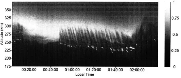
backscat-ter power data on the night of 23/24 July 2006. A dense and wavy sporadic E layer was also observed on that night. . ... . . 20
1-3 All-sky imager data for 6300
A
airglow emission recorded on the night of 23/24 July 2006, indicating a plasma structure drifting southward. 21 1-4 Summer 2006 North American heat waves as mapped by NASA'sClouds and the Earth's Radiant Energy System (CERES). The heat waves swept across from the Northwest toward the Southeast. Figure taken from Atmospheric Science Data Center [2006]. . ... 23
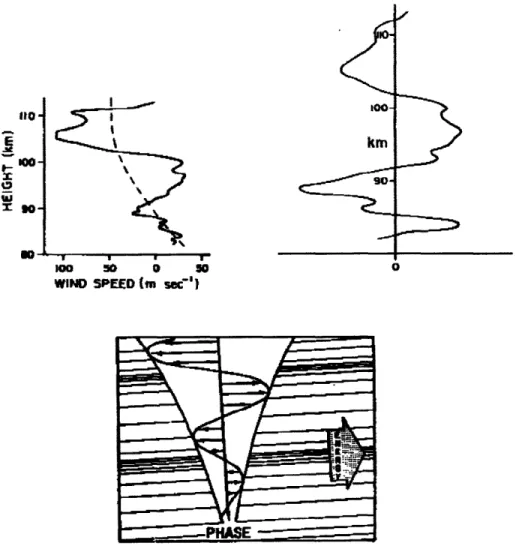
2-1 Neutral wind speed fluctuations associated with internal gavity waves at meteor heights (upper left & upper right). A pictorial illustration of internal gravity wave amplitude growth and its phase/energy
prop-agation (bottom). After Hines [1960]. ... 26
2-2 (a) A diagram showing the direction of ion motion under the influence of neutral wind in a collisional magnetized plasma. (b) Schematic illustration of the wind shear mechanism for sporadic E layer formation.
Adapted from Kelley [1989]. ... 30
2-3 Examples of Kelvin-Helmholtz billows that could develop in the spo-radic E plasma layer due to a strong wind shear. . ... 31
2-4 Sample contour plots that describe the induced plasma density fluctu-ations during the passage of internal gravity waves in the ionosphere for two different orientations of wavevector relative to the magnetic
field. Taken from Hooke [1968]. ... .. 33
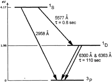
3-1 A portion of energy level diagram for atomic oxygen showing spe-cific transitions that give rise to the 5577
A
and 6300A
OI emission, which is commonly used for airglow diagnostics of ionospheric plasmas.Adapted from Carlson and Egeland [1995]. . ... 36
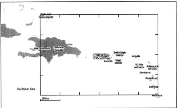
3-2 A map of Puerto Rico and the surrounding islands in the Caribbean area. The 1200 km x 800 km frame represents the coverage area of 6300
A
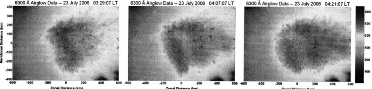
airglow measurement using ASIS at Arecibo Observatory. . . 37 3-3 Three airglow intensity maps from the night of 22/23 July 2006 whichwere recorded at 03:29:07 LT, 04:07:07 LT, and 04:21:07 LT. These airglow structures had an approximately westward direction of motion
during this time period. . ... ... 38
3-4 Airglow structure tracking analysis for the -westward moving airglow on the night of 22/23 July 2006. The airglow speed was calculated to
be 46.3 ± 2 m/s. ... ... 39
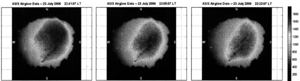
3-5 Three airglow intensity maps from the night of 23/24 July 2006 which were recorded at 22:41:07 LT, 23:05:07 LT, and 23:23:07 LT. These airglow structures had an approximately southward direction of motion
during this time period. ... 40
3-6 Airglow structure tracking analysis for the -southward moving airglow on the night of 23/24 July 2006. The airglow speed was calculated to
be 97.3 ± 7 m/s. ... ... ... 41
3-7 Three airglow intensity maps from the night of 23/24 July 2006 which were recorded at 02:13:07 LT, 02:53:07 LT, and 03:17:07 LT. These airglow structures had an approximately westward direction of motion
3-8 Airglow structure tracking analysis for the -westward moving airglow on the night of 23/24 July 2006. The airglow speed was calculated to
be 67.3 ± 5 m/s. ... .. ... 43
4-1 A schematic illustration of incoherent scatter frequency spectrum. 46 4-2 A sample ISR backscatter power profile together with the derived
iono-spheric plasma density profile. Signatures of plasma structures can be seen as dips/depletions (marked by the red arrows) in both backscatter power and plasma density profile. Note that the signatures can be seen better in the backscatter power profile. . ... . . 47
4-3 RTI plot of radar backscatter power during time period 22:30 LT -23:30 LT on the night of 22/23 July 2006, showing a slanted stripe structure at ionospheric F region altitudes. . ... 48 4-4 RTI plot of net backscatter power pertubations that correspond to
the slanted stripe structures observed on the night of 22/23 July 2006 during time period 22:30 LT - 23:30 LT. . ... 49 4-5 RTI plot of radar backscatter power during time period 01:30 LT
-03:30 LT on the night of 22/23 July 2006. A train of turbulent filaments in the F region can be seen from this data set. . ... 50 4-6 Detailed look at a specific portion of the turbulent filaments. ... 51 4-7 RTI plot of radar backscatter power during time period 22:00 LT
-23:00 LT on the night of 23/24 July 2006, showing some of the observed
slanted stripes ... 52
4-8 RTI plot of net backscatter power pertubations on the night of 23/24 July 2006 during time period 22:00 LT - 23:00 LT. In this RTI plot, four slanted stripe structures can be identified. . ... 53 4-9 RTI plot of radar backscatter power during time period 03:40 LT
-04:00 LT on the night of 23/24 July 2006, where filament structures/
4-10 RTI plot of net backscatter power pertubations on the night of 23/24 July 2006 during time period 03:40 LT - 04:00 LT. The filaments/ quasi-periodic echoes can now be seen much more clearly. Red arrow marks a particular filament that we used for slope estimation. .... 55 5-1 A diagram showing the geometry of total electron content (TEC)
mea-surements made by pairs of GPS satellite and receiver station. ... 58
5-2 Several selected plots of GPS TEC measurement made by the GPS receiver station in Isabella, PR on 23 July 2006 UTC in which TID
signatures (wavelike fluctuations in the TEC signal) were seen. ... 60
5-3 Several selected plots of GPS TEC measurement made by the GPS receiver station in St. Croix, USVI on 24 July 2006 UTC in which TID signatures (wavelike fluctuations in the TEC signal) were seen. 61 5-4 Absolute TEC measurement on 24 July 2006 UTC from GPS
satel-lite #8 by Isabella GPS receiver station (upper panel). The corre-sponding TEC perturbation (TECP) from this measurement after the background signals were removed (lower panel). . ... 63 5-5 A comparison between TECP signals from GPS receiver station in
Isabella, PR (upper panel) and St. Croix, USVI (lower panel). The red arrows mark the corresponding TID signatures that can be identified
in both TECP signals. ... ... 64
5-6 Trajectory lines of GPS satellite #8's ionospheric piercing points that correspond to TEC measurements made by Isabella and St. Croix GPS receiver stations, respectively. Also shown along these trajectories are the locations where each of the corresponding TID signatures A-E (Isabella station) and A'-E' (St. Croix station) were detected. .... 65 6-1 The geometry of plasma density striations when the TID structures
are progressing southward. . ... .... 69
6-2 The geometry of plasma density striations when the TID structures
6-3 Summary plots of space weather condition on 21-27 July 2006 from NOAA's Space Physics Interactive Data Resource (SPIDR) database [2006]. Low values of Ap and K, indices show that the geomagnetic condition was quiet during our experiment. . ... . . 72 6-4 Hurricane track map for the 2006 Atlantic hurricane season [National
Hurricane Center, 2006]. No major hurricane had passed near Puerto
Rico during our experiment. ... .. 74
6-5 The progression of summer 2006 North American heat waves on 20-25 July 2006. Data from the National Climatic Data Center, NOAA
[2006]. ... 76
7-1 North American and West European heat waves during summer 2006 as mapped by the Moderate Resolution Imaging Spectroradiometer
(MODIS) on NASA's Terra satellite [2006]. . ... . 80
A-1 A schematic description of the first two steps of the required array manipulations before a more intensive analysis can be performed on
the ASIS airglow data. ... 84
A-2 Transformations from the top-view array A3 into the geographical ar-ray G. Matrix element A3(i,j) from top-view arar-ray will become matrix element G(i',j') in geographical array. . ... 85 A-3 Basic geometry relating the height of airglow layer to the horizontal
extent of airglow measurement using an all-sky imager. . ... 86 A-4 Contour map of a sample airglow intensity data recorded using ASIS.
The image edge is located at the transition between the area where the contour is clean and the area where clusters of random dark noise start to develop. Center pixel and image radius is determined through analytical curve fitting of the image edge. . ... 88 A-5 Curve fitting results of ASIS image edge for the lower arc (left) and for
B-1 Basic schematics of the airglow structure tracking procedures. The distinctive part of airglow structure is "locked-on" first in Datafile #1. We will then locate the new position of this structure in Datafile #2 onwards by scanning the "lock-on" frame around, looking for the
best-matched pattern. ... ... .. ... 92
B-2 A sample likelihood surface plot that was obtained after scanning an ASIS snapshot. In each ASIS snaphots following the reference snap-shot, the tracked airglow structure position is found by locating the coordinate (Xi, Y) where the likelihood is maximum. . ... 93 B-3 A plot of the tracked airglow structure positions from a number of
ASIS snaphots following a particular reference snapshot. This airglow trail is the end result of the first stage in our tracking procedures. .. 94 B-4 A sample linear regression result in determining the overall airglow
motion direction from the airglow trails. Also shown in the figure is a schematic illustration of the reference point and the null point that are used in the "projection" procedures as a preliminary step for determining the speed of airglow motion. . ... 95 B-5 Determining the airglow motion speed through curve fitting. Most of
the time, we only need linear regression since the airglow motion speed
List of Tables
1.1 Arecibo ISR observation summary for our experiment on the night of
22/23 and 23/24 July 2006. ... ... 22
1.2 ASIS airglow observation summary for our experiment on the night of
22/23 and 23/24 July 2006. ... 22
A. 1 The values for the center pixel and the image radius that were obtained from the curve fitting of the image edge. Shown are the individual fitting parameter results from upper and lower arc, together with the weigthed average of the two results. . ... 89
Chapter 1
Introduction
On 21 March former US Vice President Al Gore delivered his testimony for the US House of Representatives regarding the issue of global warming and climate crisis
[Gore, 2007]. There have been indications that higher atmospheric temperatures
associated with global warming may cause various ecological effects such as the oc-currences of more intense weather anomalies and the rise of sea levels due to melting of polar cap ice. These are a few examples of observable effects on the Earth's surface (litosphere/hydrosphere) and in the lower atmosphere (troposphere). We can now ask another question: are there any effects that global warming may impose on space plasmas? This would involve regions even farther away from the Earth's surface (e.g. upper atmosphere, ionosphere, and probably magnetosphere). This thesis will dis-cuss our observation of intense ionospheric plasma disturbances that could have been closely linked to the summer 2006 US heat wave-one of the most recent indication of global warming.
1.1
Background and Motivations
Plasma turbulence is a topic of great interest in both space plasma and fusion research. In most cases, plasma turbulence is something that we want to avoid because it can pose serious problems (e.g. radio communication blackouts due to space plasma disturbances, disruptions in fusion processes). Therefore, it is important for us to
E lo
ti
td
0.75 0.5 0.25 n Local TimeFigure 1-1: Sheet-like ionospheric plasma irregularities generated by Arecibo HF heater during the 1997 heating experiment. From Lee et al. [1998].
study the nature and the source of plasma turbulence. With a good understanding on this subject matter, we would be able to prevent any potential problems from occurring.
In general, space plasma turbulence can be excited by either natural or man-made sources. Artificial space plasma disturbances are often generated during controlled-studies of space plasma using ground-based radio frequency (RF) heater, as an attempt to study various aspects of physics involved in the plasma turbulence. During the 1997 experimental campaign at the Arecibo Observatory, sheet-like plasma den-sity irregularities were formed at ionospheric F region altitudes as a result of injection of powerful high-frequency (HF) heater waves [Lee et al., 1998]. These parallel-plate structures were succesfully detected by the Arecibo incoherent scatter radar (ISR) as they drifted westward. In the radar backscatter power data, these parallel-plate structures appeared as slanted stripes, as depicted in Figure 1-1.
While Arecibo HF heater could generate artificial parallel-plate plasma structures, we also had observed a few cases of highly-structured naturally-occurring ionospheric plasma disturbances over Arecibo in our most recent (July 2006) experiments. Some of these natural ionospheric plasma disturbances were detected by the Arecibo ISR as slanted stripes, which means that they were also sheet-like plasma structures-just
like the heater-generated plasma irregularities in 1997 Arecibo heating experiment. More interestingly, these highly-structured ionospheric plasma turbulence were ob-served during geomagnetically quiet nights. It is thus a challenge for us to pinpoint the source of these disturbances. On the bright side, however, we might be able to identify new interesting sources that had not been noticed before.
1.2
Summary of The Observed Phenomena
During our experimental campaign at the Arecibo Observatory on 21-27 July 2006, we observed a very turbulent ionosphere on some of the nights. Based on the data from our diagnostics instruments, there had been some indications of a turbulent plasma state at the beginning of our experiment, prior to the occurrence of fully-developed turbulent plasma structures.
First, ionosonde measurement shows that the ionospheric F region peak plasma frequency early in the evening was quite high (around 8 MHz or so) on most nights. This was unusual because we are currently in the solar minimum. High plasma density early in the evening indicates that recombination process in the F region was very slow at that time. From the all-sky imager data, we also observed a post-twilight enhancement for the 6300
A
airglow emission on those nights, which confirmed that the recombination rate in the ionospheric F region was indeed very slow at that time. High plasma density in general will lower the threshold for various plasma instabilities in the ionosphere.Second, shortly after the F region peak plasma frequency fall into its normal nighttime value (around 3-4 MHz) later in the evening, sharp density gradients often formed at the bottomside ionosphere. This will enhance the possibility for the (gener-alized) Rayleigh-Taylor instability to develop. Following the formation of this sharp density gradient, often there was also some intermediate (peel-off) plasma layers that separated and descended from ionospheric F region into E region altitudes.
Finally, we also observed intense sporadic E plasma layers around an altitude of 110-120 km, with wavelike structures embedded in those layers. This would be an
in-450 400 350 E S300 250 200 150 100
Arecibo ISR Backscatter Power Profile (RTI Display) Date: 23/24 July 2006
22:00 22:30 23:00 23:30 00:00 00:30
Local Time (hours)
Figure 1-2: The observed slanted stripes on the RTI display of Arecibo ISR backscat-ter power data on the night of 23/24 July 2006. A dense and wavy sporadic E layer was also observed on that night.
dication of a strong neutral wind shear which formed the layer and excite the wavelike structures via Kelvin-Helmholtz instability. The presence of such strong neutral wind shear also implies an intense perturbation in the neutral atmosphere, most likely in the form of internal gravity waves, that could even couple into ionospheric F region plasmas and produce some traveling ionospheric disturbances (TID).
One of the most prominent plasma structures that we observed was the slanted stripe pattern that appeared on the night of 23/24 July 2006, as shown in the Range-Time-Intensity (RTI) plot of Arecibo ISR data (Figure 1-2). These slanted stripes, which appeared for almost 3 hours in the Arecibo ISR data, were downward-sloping. Such slanted stripe pattern is typically caused by sheet-like plasma structures that move across the radar beam. Since plasma density irregularities must be field-aligned and because the radar beam was pointed vertically during our experiment, then we may deduce that these sheet-like plasma structures were tilted following the magnetic
1400 t200 1000
800 200
Figure 1-3: All-sky imager data for 6300 A airglow emission recorded on the night of 23/24 July 2006, indicating a plasma structure drifting southward.
dip angle (-50' at Arecibo) while drifting southward and downward perpendicularly across the magnetic field lines. This is one of the simplest configuration that will result in downward sloping stripes in the RTI plot of Arecibo ISR data.
The above conjecture was also consistent with the airglow measurement made by our all-sky imager. In the 6300
A
airglow data, we observed an airglow structure which moved in the -southward direction during the time period of interest. Depicted in Figure 1-3 is a sequence of all-sky imager data that shows this southward airglow motion. The 6300 A airglow emission originates from altitude range of 250-300 km, which largely coincides with the altitude range of the observed slanted stripes.There are a few other cases of turbulent plasma structures that we had observed during our July 2006 campaign at the Arecibo Observatory, as well. We are going to discuss them in detail in later chapters of this thesis. The data presentation of these turbulent plasma structures is going to include both airglow diagnostics (Chapter 3) and ISR diagnostics (Chapter 4). A short summary of radar and airglow observation that we are going to report in this thesis can be found in Table 1.1 and Table 1.2, respectively.
In addition, we are also going to present some GPS TEC data from these two nights in Chapter 5. The GPS TEC diagnostics is particularly useful for identifying TID signatures, and can be extended to provide 2-D map of ionospheric plasma disturbances [Rideout and Coster, 2006; Nicolls et al., 2004]. The results from each diagnostics are finally going to be reconciled and combined to provide a complete picture of these plasma disturbances. The combined analysis is going to be presented
A•lfi•,4~nl~· u~-)~* rtll - •t.hi 9• 13 •.4.r7 ASlK Airniautw nsJlr--•Jul•t 1 •3•671 A•I• Airnlaw Irlt -- 9ul••*"2ýn7 dL T
Table 1.1: Arecibo ISR observation and 23/24 July 2006.
summary for our experiment on the night of 22/23
Date / Time Period Description ASIS Data Supportt
NIGHT OF 22/23 JULY 2006
22:30 LT - 23:30 LT Slanted stripe NO
01:30 LT - 03:30 LT Train of turbulent filaments YES
NIGHT OF 23/24 JULY 2006
21:30 LT - 00:45 LT Slanted stripes YES
03:40 LT - 04:00 LT Quasi-periodic echoes/filaments YES
tThis indicates whether any recognizable airglow structure motion was seen in the ASIS airglow data.
Table 1.2: ASIS airglow observation summary for our experiment on the night of 22/23 and 23/24 July 2006.
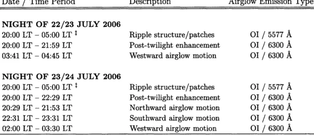
Date / Time Period Description Airglow Emission Type
NIGHT OF 22/23 JULY 2006
20:00 LT - 05:00 LT t Ripple structure/patches OI / 5577 A
20:00 LT - 21:59 LT Post-twilight enhancement OI / 6300
A
03:41 LT - 04:45 LT Westward airglow motion OI / 6300
A
NIGHT OF 23/24 JULY 2006
20:00 LT - 05:00 LT ' Ripple structure/patches OI / 5577
A
20:00 LT - 22:29 LT Post-twilight enhancement OI / 6300
A
20:29 LT - 21:53 LT Northward airglow motion OI / 6300
A
22:31 LT - 23:31 LT Southward airglow motion OI / 6300 A
02:00 LT - 03:30 LT Westward airglow motion OI / 6300
A
North American Heat Waves (July 2006 - Ai
Ou1gong LongoWa Rodiin (wim)2
160 320
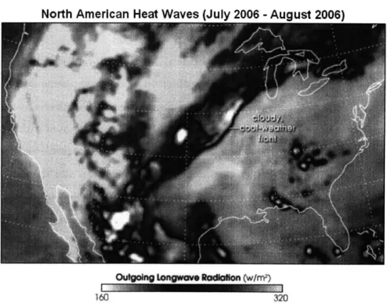
Figure 1-4: Summer 2006 North American heat waves as mapped by NASA's Clouds and the Earth's Radiant Energy System (CERES). The heat waves swept across from the Northwest toward the Southeast. Figure taken from Atmospheric Science Data
Center [2006].
in Chapter 6 of this thesis.
1.3
Proposed Hypothesis
We strongly believe that the observed ionospheric plasma turbulence must have been caused by internal gravity waves that had reached ionospheric F region altitudes. One reason is that, as briefly discussed in the previous section, we had also observed some wavy sporadic E plasma layers during our July 2006 experiment. This observation indicates a strong perturbation in neutral atmosphere during that period of time, which is very likely to be in the form of internal gravity waves. Thus, our task has finally been narrowed down to finding the source of these gravity waves.
As also briefly mentioned before, the geomagnetic condition was generally quiet during our July 2006 Arecibo experiment. This implies that auroral activity cannot
possibly be the source of these gravity waves. Hence, we have to look for gravity wave source that is either terrestrial or meteorological in origin.
We suspect that the summer 2006 US heat wave was the responsible source of gravity waves that subsequently excite the observed ionospheric plasma disturbances over Arecibo. As it swept across the United States from the Northwest toward the Southeast, there had been reports on severe weather events associated with the heat wave. It is thus possible that upon leaving the shore, the heat wave then further seeded more atmospheric disturbances over the Gulf of Mexico and the Caribbean. Figure 1-4 shows the summer 2006 US heat wave, based on the amount of long wave radiation from the Earth's surface, as mapped by NASA's Clouds and the Earth's Radiant Energy System (CERES) [ASDC, 2006].
It should be noted that no other nearby weather anomalies could have been re-sponsible for the observed ionospheric plasma disturbances. First of all, there was no close encounter of hurricanes near Puerto Rico around the time of our observation. Furthermore, there was no other major catastrophic weather event such as volcano eruptions, earthquakes, or tsunamis-which had been known as powerful source of strong gravity waves in the Earth's atmosphere. The absence of such "conventional" gravity wave sources leads us to focus our attention to the summer 2006 US heat wave, which was the most relevant weather anomaly in terms of its timing and lo-cation. Detailed discussion on the search of the responsible gravity wave source is presented in Chapter 6 of this thesis.
The above speculation has the implication that global warming-related events might have real and significant effects on space plasmas, even though this type of plasmas are located very far away from the Earth's surface. This certainly warrant further investigation and scrutiny. An outline of planned future work to further investigate this phenomenon is given in Chapter 7 along with the conclusion of the current work.
Chapter 2
Ionospheric Disturbances:
An Overview
This chapter is going to provide some background information on gravity waves and the related ionospheric plasma disturbances. This is particularly relevant for our current study of ionospheric plasma turbulence in the mid-latitude regions, because gravity waves are often the cause of plasma turbulence there.
Gravity waves are important in mid-latitude ionospheric studies for the follow-ing reason. Unlike in polar or equatorial regions, magnetic field configuration in mid-latitudes is not conducive to the Rayleigh-Taylor instability and auroral current usually does not reach that far except during severe substorms. Thus, other types of source mechanism usually drive plasma turbulence in mid-latitudes. When there exist some disturbances in the neutral atmosphere, internal gravity waves could pro-vide coupling between neutral atmosphere and the ionosphere. By carrying energy away from lower atmosphere and dissipate it in the ionosphere, gravity waves would subsequently trigger plasma turbulence [Lastovicka, 2006].
2.1
Internal Gravity Waves
Gravity waves are disturbances in the atmosphere that usually appear as neutral wind fluctuations. The magnitude of these wind fluctuations might not be very
00 -WJ X 90 IN o0-km - 1o 1WI 50 0 50
WIND SPEED (m seC')
Figure 2-1: Neutral wind speed fluctuations associated with internal gavity waves at meteor heights (upper left & upper right). A pictorial illustration of internal gravity wave amplitude growth and its phase/energy propagation (bottom). After Hines
[1960].
significant near the ground, but they could be far more noticeable when they had reached the upper atmosphere. The two upper graphs in Figure 2-1 show an example of horizontal neutral wind speed fluctuation at meteor heights due to internal gravity waves. It should be noted that even in the absence of gravity waves, a background wind velocity profile/shear could still exist in the upper atmosphere (shown as dashed lines in the upper left graph of Figure 2-1). Thus, background wind profile and the wind fluctuations due to gravity waves will typically be superposed on top of each other. The upper right graph in Figure 2-1 shows the net wind fluctuations associated with the gravity waves, without the background wind profile contribution.
I> r
t
Roughly speaking, atmospheric gravity waves can be divided into two categories: (1) internal gravity waves and (2) surface waves. The difference between the two lies in their capability of having vertical propagation [Hines, 1960; Yeh and Liu, 1972]. Internal gravity waves could support a substantial vertical propagation, while surface waves are evanescent along vertical direction. Internal gravity waves are the ones of interest to us because we will be dealing with coupling processes between neutral atmosphere and the ionosphere. We shall next look into some defining features of internal gravity waves.
There are several important features of internal gravity waves [Hines, 1960; Nappo, 20021. First of all, internal gravity waves need to have wave periods larger that a cer-tain characteristic value given by -r, _ 2 Otherwise, the internal wave will become evanescent. Here c, denotes the speed of sound; g is the gravitational accel-eration; and 7 is the ratio of specific heats. Furthermore, the amplitude of internal gravity waves tends to increase (oc exp[•j]) as they propagate upwards because at-mospheric density generally decreases with altitudes. This is a direct consequence of energy flux conservation during gravity wave passage in the atmosphere. Another interesting feature of internal gravity wave is that the direction of phase propagation is nearly perpendicular to the direction of energy propagation (i.e., phase velocity is -perpendicular to group velocity). Some of these features are illustrated in the bottom graph of Figure 2-1: The growth of gravity wave oscillation amplitudes can be seen from the enveloped arrows of wind velocity vectors. In the case shown here, the energy propagation is obliquely upwards and the phase propagation is almost vertically downward.
A dispersion relation that describes internal gravity waves has been derived by
Hines [1960], and it is given by (assuming an isothermal atmosphere):
w4 _ 2c (k + k ) (Y _ 1)g2k -) = 0 (2.1)
where c, is the sound speed; g is the gravitational acceleration; - is the ratio of specific heats; w is the wave frequency; and kx (k,) denotes the horizontal
(verti-cal) wavenumber, respectively. The roots of the above quartic equation in w di-vide this wave mode into two regimes: a high-frequency branch and a low-frequency branch. The high-frequency branch has wave frequencies w > w, - 7g/2c8, and is
termed acoustic waves. Meanwhile, the low-frequency branch has wave frequencies
w < Wb =- - g/cs, and it is the internal gravity waves. For any intermediate fre-quencies Wb < w < wa, no internal gravity wave modes are allowed. The characteristic frequency wb is known as the Brunt-Vaisala frequency, which is the natural frequency for air parcels in the atmosphere to oscillate up and down due to buoyancy [Kelley,
1989; Yeh and Liu, 1972].
The dissipation of internal gravity waves primarily depends on two atmospheric properties: viscosity and thermal conductivity [Hines, 1960; Yeh and Liu, 1972]. Dissipation generally becomes important at greater heights, such as in the upper atmosphere or the ionosphere. This is where internal gravity waves finally break apart and dissipate energy after growing in amplitudes. Furthermore, the dissipation turned out to be more severe for internal gravity waves with smaller scale/wavelength. In other words, internal gravity waves with smaller scale/wavelength would be dissipated at lower altitudes compared to larger-scale gravity waves.
2.2
Sporadic-E Plasma Layer and Kelvin-Helmholtz
Instability
Sporadic E layers are thin, patchy, yet dense plasma layers in the ionospheric E re-gion at around 100-120 km altitudes. In the mid-latitudes, sporadic E layers are formed by neutral wind shear in the upper atmosphere. Typically, zonal (east-west) wind shear is more effective in creating sporadic E layers compared to meridional (north-south) wind shear [Kelley, 1989]. The wind shear itself might be due to in-ternal gravity waves, which makes the presence of sporadic E layers an indication of gravity wave occurrences. Furthermore, if the wind shear is strong enough, plasma structures/irregularities could subsequently develop in the sporadic E layer
[Bern-hardt, 20021. This is likely due to a type of magnetohydrodynamic (MHD) instability
known as the Kelvin-Helmholtz instability.
We will now discuss the wind shear mechanism for sporadic E layer formation. We begin the analysis by writing down the ion momentum equation (for a particular
ion species j):
P
a.
+(V13 .V) 3)=-Vp+pj + njqj(E + vj xB)--•pjVjk(fj- -Vk) (2.2)t k
where pj denotes the ion mass density, p is the pressure, ' is the gravitational accel-eration vector, nj is the ion number density, qj is the ionic charge, E is the electric field, B is the magnetic field, and vik is the collision frequency between species j and
k. Assuming steady-state condition, we can set the LHS of Equation 2.2 to be zero.
Furthermore, we will only consider collisions with neutral particles (i.e., the index k will represent the neutral particles). We will also ignore pressure gradient, gravity, and any electric field. We then have:
o
=o
+
nie(O + i x B) - piVin(( - n)Pivin(i -Un) = nie(i B x ) (2.3)
where Un represent the background neutral wind velocity, and we have assumed singly-ionized ions. The background magnetic field is assumed to be constant and uniform everywhere. Meanwhile, the neutral wind velocity is chosen to be flowing perpendic-ularly to the magnetic field lines, and have no time dependence.
We will adopt a coordinate system where the magnetic field is pointing in the i direction, and the background neutral wind is flowing along the i direction. Then the vector quantities can be written explicitly as n, = [Un, 0, 0]; B = [0, 0, B]; and
i = [vix, vi7, viz]. Let us define n - eB/Mivin where Mi is the ion mass. Also recall
NEUTRAL WIND , B® - f
foNS
B( U -_ PLASMA () M NU SU x ACCUMULATIONS Vi 0 IONS, / / . NEUTRAL WIND Y (a) (b)Figure 2-2: (a) A diagram showing the direction of ion motion under the influence of neutral wind in a collisional magnetized plasma. (b) Schematic illustration of the wind shear mechanism for sporadic E layer formation. Adapted from Kelley [1989].
definition, we will obtain:
n[2vy, -vi,, 0] = [vi, - U), vi, viz] (2.4)
which forms a system of equations for vij, viy, and viz. Solving these coupled
equa-tions, we will have:
Un
Un
vi = -1+ 2 ; = 2 vi =0 (2.5)
for the ion velocity components. The results given in Equation 2.5 thus give a general idea on how the ions will move as a response to a constant background neutral wind in a collisional magnetized plasma.
Figure 2-2(a) give a graphical illustration of the resulting ion motion as described by Equation 2.5. As shown in this figure, the ions will be dragged by the neutral wind, but because of the magnetic Lorentz force, the ion motion will be deflected sideways from the original neutral wind direction. For opposite neutral wind directions, the direction of the resulting ion motion will be reversed as well. Now consider a case where neutral wind at two different altitudes are in opposite directions (an example of wind shear) as depicted in Figure 2-2(b). In the configuration shown here, ions from higher altitudes will be deflected downwards and vice versa. As a consequence, the ions will be accumulated at the center-in between these sheared streams. The electrons will subsequently follow the ions to accumulate there, thus maintaining the overall charge neutrality. This is the wind shear mechanism for the formation of
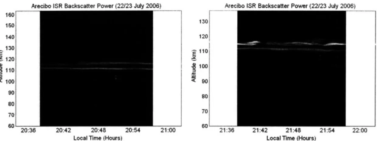
160 150 140 130 120 110 100 90 80 70 an
Arpaihn IRR R ak-cattpr Power (21/23 July 2001S
20:36 130 120 110 * 100 90 80 70 an 21:00 21:36 21:42 21:48 21:54 22:00
Local Time (Hours) Local Time (Hours)
Figure 2-3: Examples of Kelvin-Helmholtz billows that could develop in the sporadic E plasma layer due to a strong wind shear.
sporadic E plasma layers in mid-latitude regions [Kelley, 1989].
If we have a sufficiently strong wind shear, some wave structures might also develop in the sporadic E layers due to Kelvin-Helmholtz instability. This instability is driven by velocity shear and it could develop in neutral fluids as well as in plasmas.
An analysis of Kelvin-Helmholtz instability in plasmas using incompressible ideal MHD equations had been discussed by Siscoe [1983]. The analysis considered two plasma regions that are separated by a tangential discontinuity in fluid velocity, den-sity, and magnetic field. Wave fluctuations in the boundary/interface could grow via Kelvin-Helmholtz instability if a threshold condition is satisified:
(Ai. k)2> -
1
[(B1.)
+ (B2 2" ] (2.6)where AV' is the difference in plasma fluid velocity across the interface; k denotes the wavevector of the fluctuations; p1 (P2) denotes the mass density in region 1 (region 2); and B1 (B2) denotes the magnetic field in region 1 (region 2), respectively. Once the instability is excited and eventually saturates, there would be a dominant wavenumber that determine the characteristic wavelength of the fully-developed Kelvin-Helmholtz modes. During experiments, we would typically see this characteristic wavelength only.
Figure 2-3 shows some examples of wavy and intense sporadic E layers that we
-I Arecibo ISR Rankqeatter Power (2•013 0July M061·~,
-observed during the July 2006 experimental campaign at the Arecibo Observatory. Wavelike fluctuations in those plasma layers are presumably Kelvin-Helmholtz modes that were driven by a strong wind shear. The neutral wind fluctuations causing the shear might have been associated with internal gravity waves. Thus, the existence of wavy and intense sporadic E layers on that night was probably an early indication of strong internal gravity waves entering the ionosphere from the lower atmosphere.
2.3
Ionospheric Disturbances Induced by Gravity
Waves
In addition to neutral wind fluctuations, there are also neutral density and pres-sure fluctuations associated with internal gravity waves. Due to interactions between plasma and neutral particles, some plasma density fluctuations in the ionosphere could be generated as gravity waves propagate through. The induced plasma fluctu-ations are usually referred to as traveling ionospheric disturbances (TID). It should be noted, however, that wavefronts of the induced TID might not necessarily coincide with wavefronts of the gravity waves. The movement of TID might also be different from the propagation direction of the inertial gravity waves. This is because charged particle motions are restricted by the Earth's magnetic field while neutral particles are not. Since TIDs are plasma disturbances, their movement will generally follow
Ex B drift.
Fluctuations in neutral particle density and pressure could significantly affect ion production rate and plasma recombination rate in the ionosphere. This is the main reason for the formation of plasma density perturbations in the ionosphere during the passage of internal gravity waves. An early theoretical foundation for this process was carried out by Hooke [1968]. This basic model for the gravity wave-induced TIDs had implemented the above ideas on how neutral density perturbation affects ion production and recombination.
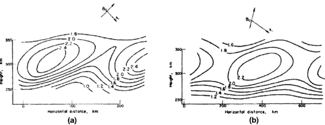
/; Ae -3O I '2~N .~ L4 ...
"irnfiol 4'tarnce. km Wwrzonfol ditsaiCe. km
(a) (b)
Figure 2-4: Sample contour plots that describe the induced plasma density fluctua-tions during the passage of internal gravity waves in the ionosphere for two different orientations of wavevector relative to the magnetic field. Taken from Hooke [1968].
The expression for the induced electron plasma density fluctuation as calculated by Hooke [1968] is given by:
6Ne(x, y, z, t) = Neo(Z) Ub(zo) sin I exp[k,,,m(z - zo)] A ,) s n \)
x exp i wt - kx - ky - kz + - tan- sin I (_k_ b
+
k~)2 NoO
+k,
where zo is an arbitrary reference height; Ub is the amplitude of wind fluctuations along the magnetic field; I is the magnetic dip angle; kb -- - B is the projection of
gravity wave wavevector along the magnetic field; and subscripts Re (Im) indicates the real (imaginary) part, respectively. Figure 2-4 shows two examples of the cal-culated plasma density perturbations based on this model. Both cases describe the situation for mid-latitude regions where the neutral wind fluctuations is in the order of -100 m/s. Figure 2-4(a) is the case where the wavevector is exactly perpendicular to the magnetic field lines, whereas Figure 2-4(b) is the not-exactly-perpendicular case.
As one can see, the resulting plasma density perturbations might not be exactly aligned with the gravity wave wavefronts. Nonetheless, if the overall phase progression of gravity waves had a downward component then typically so did the plasma density
VE
2rO
striations. The TID configuration therefore would mimic the phase progression of inertial gravity waves to some extent. Hence, judging from their configuration, TIDs with geometry of slanted plasma sheets/stripes are probably the ones triggered by inertial gravity waves from neutral atmosphere.
Chapter 3
Airglow Diagnostics
Presented in this chapter are the results of airglow measurement using MIT All-Sky Imaging System (ASIS) performed on the night of 22/23 and 23/24 July 2006 at Arecibo Observatory, Puerto Rico. There was no (or very few) clouds on these two nights, thus giving us an opportunity to utilize airglow diagnostics using an all-sky imager to its fullest potential. This chapter is going to begin with a brief overview of using airglow measurement to diagnose ionospheric plasma turbulence, followed with a thorough data presentation from the two nights of succesful airglow measurements.
3.1
Ionospheric Plasma Diagnostics Through Airglow
Measurement
Lights that are emitted by atoms/molecules from the Earth's atmosphere can in principle be observed, and they are known as airglows. Although airglow is difficult to observe during the daytime, the nighttime airglow can be observed much more easily and we can obtain a good diagnostics on ionospheric plasma turbulence by looking at airglow structures using an all-sky imager. Airglow measurement using an all-sky imager has a great advantage due to its capability to map the turbulent ionospheric structures in 2-D, giving us a clear picture of the situation.
AXI 4.17 1.96 n 1D 363 A
Figure 3-1: A portion of energy level diagram for atomic oxygen showing specific tran-sitions that give rise to the 5577
A
and 6300A
OI emission, which is commonly used for airglow diagnostics of ionospheric plasmas. Adapted from Carlson and Egeland[1995].
inside atoms/molecules. Thus, specific emission lines usually characterize specific re-gions of the ionosphere where the population density of a particular atomic/molecular species is dominant, and where a particular energy level transition occurs at a signif-icantly fast rate. The two commonly used emission lines for diagnosing ionospheric plasma are the 5577 A (green) and 6300 A (red) OI (neutral atomic oxygen) emis-sion. The 5577 A OI emission mainly originated from -90 km altitude, around the ionospheric E-region, whereas the 6300
A
OI emission comes from the ionospheric F-region (around 250-300 km altitude). Figure 3-1 illustrates the specific energy level transitions inside neutral atomic oxygen that give rise to the 5577 A and 6300A
OI emission.The 6300 A emission is mainly caused by a chain of chemical reactions in the ionospheric F-region, started with molecular ion formation through [Chamberlain,
1961]
0+ + 02 -- O + O (3.1)
and followed by dissociative recombination process
O+ + e- --, O* + O* (3.2)
Figure 3-2: A map of Puerto Rico and the surrounding islands in the Caribbean area. The 1200 km x 800 km frame represents the coverage area of 6300
A
airglow measurement using ASIS at Arecibo Observatory.where O* indicates neutral atomic oxygen in its excited state. The excited O* then relaxes to a lower energy state, emitting the 6300
A
photon. Alternatively, the molec-ular ion formation can also occur in a different way [Chamberlain, 1961]:0+ + N2--+ NO + + N (3.3)
which is then followed by the following dissociative recombination:
NO++ e- -+ N* + O* (3.4)
Meanwhile, the origin of 5577
A
OI emission is the reaction [Chamberlain, 1961]O + O + O -, 02 + O(
1S)
(3.5)and it is suppressed by collisional de-excitation through the reaction
4 3 -2
ii
I
I
i0 400 1200 100Zornd •81€o |km) Z DismW (k) Zod DWrro (km)
Figure 3-3: Three airglow intensity maps from the night of 22/23 July 2006 which were recorded at 03:29:07 LT, 04:07:07 LT, and 04:21:07 LT. These airglow structures had an approximately westward direction of motion during this time period.
where N2 is left in a vibrational excited state.
In this thesis, we will be focusing on the 6300
A
airglow emission for the diagnos-tics of ionospheric F-region plasma turbulence. Figure 3-2 schematically shows the geographical area that is covered by the all-sky imager's field of view for the 6300A
airglow measurement. All airglow intensity maps presented in this chapter have been transformed into geographic coordinates with linear distances (kilometers) along zonal and meridional directions. The detailed description of coordinate tranformation from an all-sky image into a geographic airglow map can be found in Appendix A of this thesis.
3.2
All-Sky Airglow Measurement on The Night
of 22/23 July 2006
During the night of 22/23 July 2006, the sky was overall clear even though there were a few cloud patches right after sunset and shortly before sunrise. On this night, an overall westward motion of airglow was observed during time period 03:41 LT - 04:45 LT. Figure 3-3 shows three sequential airglow intensity maps recorded by ASIS at 03:29:07 LT, 04:07:07 LT, and 04:21:07 LT which illustrate this westward motion.
A further analysis to track the motion of the observed airglow structures was also performed to determine its actual speed and direction of motion. The detailed procedures for the airglow structure tracking can be found in Appendix B of this
50 0 -50 -100 -150 -200 -250
ASIS Airglow Structure Tracking 22/23 July 2006
-150 -100 -50
X (km)
100
Figure 3-4: Airglow structure tracking analysis for the -westward moving airglow on the night of 22/23 July 2006. The airglow speed was calculated to be 46.3 ± 2 m/s.
thesis. Figure 3-4 shows the result of this analysis. The fitted straight-line trajectory tells us that the airglow motion was toward the 281.30 direction (11.3' north of west). The airglow strutures started to spread apart toward north and south as it progressed westward, thus causing more uncertainty in the exact direction of airglow. Nonetheless, a result of overall -westward direction was established from this analysis. The speed of this airglow motion was determined to be approximately 46.3 m/s, with an uncertainty of -2 m/s. 03:41:07 LT _______Ia El _ Ell M ---.- -04:45:07 LT . . . . . . . . . . . ar . ..r m ,t a• rr r r
I
I
000 · 00 100 00 00 SooZo"n W o (kin) Zoed JWuo. (kin) Zono Dloboo (km)
Figure 3-5: Three airglow intensity maps from the night of 23/24 July 2006 which were recorded at 22:41:07 LT, 23:05:07 LT, and 23:23:07 LT. These airglow structures had an approximately southward direction of motion during this time period.
3.3
All-Sky Airglow Measurement on The Night
of 23/24 July 2006
During the night of 23/24 July 2006, a richer airglow motion pattern was observed. The sky condition was also much better than the night before, with absolutely no cloud patches interrupting our observations. Presented in this section are the analysis of two different airglow structures that were observed at two distinct period of time. Earlier that night, a southward airglow motion was observed; whereas later that night, a westward airglow motion was observed.
3.3.1
Observation of a Southward Airglow Motion
During the night of 23/24 July 2006, a -southward motion of airglow was observed during time period 22:31 LT - 23:31 LT. Figure 3-5 shows three sequential airglow intensity maps recorded by ASIS at 22:41:07 LT, 23:05:07 LT, and 23:23:07 LT which illustrate this southward motion.
A further analysis to track the motion of the observed airglow structures was again performed to determine its actual speed and direction of motion. Figure 3-6 shows the result of this airglow tracking procedures. From the fitted straight-line trajectory,
we found that the airglow motion was toward the 170.10 direction (9.90 east of south).
The airglow motion was quite firm, so that only a relatively small uncertainty of -0.450 was affecting the result for the direction of motion. The speed of this southward
"cnfl LUU
150
100
50
..
0
-50
-100
-150
ASIS Airglow Structure Tracking 23/24 July 2006
-150
-100
-50
0
50
100
150
200
X (km)
Figure 3-6: Airglow structure tracking analysis for the '-southward moving airglow on the night of 23/24 July 2006. The airglow speed was calculated to be 97.3 ± 7 m/s.
airglow motion was determined to be approximately 97.7 m/s, with an uncertainty of -7 m/s. This value of airglow motion speed is the largest one of all three airglow structure motion analysis that are discussed in this thesis. In fact, this southward airglow motion coincides with the observation of a train of slanted stripes/ parallel plate structures on the Arecibo ISR backscatter power profile.
I
I
700 300 200 100ZonlW Dse (km) on D tM o J(km) Zad owco ("In)
Figure 3-7: Three airglow intensity maps from the night of 23/24 July 2006 which were recorded at 02:13:07 LT, 02:53:07 LT, and 03:17:07 LT. These airglow structures had an approximately westward direction of motion during this time period.
3.3.2
Observation of a Westward Airglow Motion
During the night of 23/24 July 2006, a 'westward motion of airglow was observed during time period 02:00 LT - 03:30 LT. Figure 3-7 shows three sequential airglow intensity maps recorded by ASIS at 02:13:07 LT, 02:53:07 LT, and 03:17:07 LT which illustrate this westward motion.
The airglow structure tracking analysis was also performed for this period of time to determine the airglow's actual speed and direction of motion. Figure 3-8 shows the result of the airglow tracking procedures. From the fitted straight-line trajectory,
we found that the airglow motion was toward the 256.50 direction (13.50 south of
west). The tracking procedures did not work too well for this set of data, and a large uncertainty of - 110 is affecting this result. From linear regression of the data points, the speed of this westward airglow motion was determined to be approximately 67.3 m/s, with an uncertainty of -5 m/s. This westward-moving airglow coincides with the observation of some filament structures/ quasi-periodic echoes from the ionospheric F-region as shown in the Arecibo ISR backscatter power profile data.
ASIS Airglow Structure Tracking 23/24 July 2006 02:17:07 LT 03:13:07 LT i % m MI i . ... .. . . 0 50 100 150 200 250 300 X (km) Figure 3-8: Airglow structure
the night of 23/24 July 2006.
tracking analysis for the -westward moving airglow on The airglow speed was calculated to be 67.3 ± 5 m/s. 300
200
100
-100
Chapter 4
Incoherent Scatter Radar
Diagnostics
This chapter will be dealing with ionospheric plasma diagnostics using incoherent scatter radar (ISR) that had been used at the Arecibo Observatory, Puerto Rico. We will begin with a brief overview regarding the basics of this diagnostics. Then, we are going to discuss the result of our ISR observation at the Arecibo Observatory on the night of 22/23 July 2006 and 23/24 July 2006 when turbulent plasma structures in the form of slanted stripes/parallel plates and filaments were observed.
4.1
Overview of ISR Measurement Basics
In diagnosing ionospheric plasmas, an incoherent scatter radar (ISR) relies primarily on the scattering of radio waves by plasma density fluctuations that are associated with ion-acoustic and Langmuir waves. In laboratory/ fusion plasmas, this type of diagnostics is usually referred to as the collective Thomson scattering diagnostics. Nonetheless, the terminology incoherent scatter is retained in space plasma commu-nity for various reasons.
The frequency spectrum of typical backscattered radar signals is schematically shown in Figure 4-1. Portion of the backscattered signals due to ion-acoustic waves is called the ion line, and it shows up as the double-humped part of the spectrum
PLASMA LINE Density PLASMA LINE Ion Accoustic Frequency SElectron Plasma Frequency \ Frequency Shift
Figure 4-1: A schematic illustration of incoherent scatter frequency spectrum.
(Doppler spreading due to thermal motion of ions). Meanwhile, the other portion due to Langmuir waves is called the plasma line, and it will show up as a sharper peak at around the electron plasma frequency. The right hand part of the graph (positive Doppler frequency shift) corresponds to scattering by electrostatic waves that propagate downward (towards the radar), and the left hand part of the graph is due to the upgoing electrostatic waves. Most of the backscattered power comes within the ion line spectrum, and a much smaller amount of power is contained in the plasma line spectrum [Dougherty and Farley, 1960; Farley, Dougherty and Barron, 1961; Bauer, 1975].
For determining ionospheric plasma density profile, one will only need the ion line portion of the incoherent scatter spectrum (since most of the backscattered power is contained there). This type of ISR operation is known as backscatter power measure-ment. The required radar receiver bandwidth for backscatter power measurement is fairly small because the width of the ion line itself is only a few ion-acoustic frequen-cies. The signal-to-noise ratio in the ion line signals is also quite high, so we only need a relatively short integration time for backscatter power measurement. The Arecibo 430 MHz ISR typically requires -10 seconds integration time for each backscatter power profile.
Shown in the left part of Figure 4-2 is a sample backscatter power measurement using Arecibo ISR on the night of 22/23 July 2006. Note that the received radar power will fall as the square of altitude/range, so that a range-squared correction will