Continuous relaxation to over-constrained temporal plans

Continuous Relaxation to Over-constrained

Temporal Plans

by

Peng Yu

B.Eng., Hong Kong University of Science and Technology (2010)

Submitted to the Department of Aeronautics and Astronautics

in partial fulfillment of the requirements for the degree of

Master of Science in Aeronautics and Astronautics

at the

MASSACHUSETTS INSTITUTE OF TECHNOLOGY

February 2013

c

Massachusetts Institute of Technology 2013. All rights reserved.

Author . . . .

Department of Aeronautics and Astronautics

January 25, 2013

Certified by . . . .

Brian C. Williams

Professor

Thesis Supervisor

Accepted by . . . .

Eytan H. Modiano

Chairman, Department Committee on Graduate Theses

Continuous Relaxation to Over-constrained Temporal Plans

by

Peng Yu

Submitted to the Department of Aeronautics and Astronautics on January 25, 2013, in partial fulfillment of the

requirements for the degree of

Master of Science in Aeronautics and Astronautics

Abstract

When humans fail to understand the capabilities of an autonomous system or its environmental limitations, they can jeopardize their objectives and the system by asking for unrealistic goals. The objective of this thesis is to enable consensus be-tween human and autonomous system, by giving autonomous systems the ability to communicate to the user the reasons for goal failure and the relaxations to goals that archive feasibility. We represent our problem in the context of temporal plans, a set of timed activities that can represent the goals and constraints proposed by users. Over-constrained temporal plans are commonly encountered while operating autonomous and decision support systems, when user objectives are in conflict with the environment. Over constrained plans are addressed by relaxing goals and or con-straints, such as delaying the arrival time of a trip, with some candidate relaxations being preferable to others. In this thesis we present Uhura, a temporal plan diagnosis and relaxation algorithm that is designed to take over-constrained input plans with temporal flexibility and contingencies, and generate temporal relaxations that make the input plan executable. We introduce two innovative approaches within Uhura: collaborative plan diagnosis and continuous relaxation. Uhura focuses on novel ways of satisfying three goals to make the plan relaxation process more convenient for the users: small perturbation, quick response and simple interaction.

First, to achieve small perturbation, Uhura resolves over-constrained temporal plans through partial relaxation of goals, more specifically, through the relaxation of schedules. Prior work on temporal relaxations takes an all-or-nothing approach in which timing constraints on goals, such as arrival times to destinations, are com-pletely relaxed in the relaxations. The Continuous Temporal Relaxation method used by Uhura adjusts the temporal bounds of temporal constraints to minimizes the perturbation caused by the relaxations to the goals in the original plan.

Second, to achieve quick responses, Uhura introduces Best-first Conflict-directed Relaxation, a new method that efficiently enumerates alternative options in best-first order. The search space of alternative options to temporal planning problems is very large and finding the best one is a NP-hard problem. Uhura empirically demonstrates fast enumeration by unifying methods from minimal relaxation and conflict-directed

enumeration methods, first developed for model based diagnosis. Uhura achieves two orders of magnitude improvement in run-time performance relative to state-of-the-art approaches, making it applicable to a larger group of real-world scenarios with complex temporal plans.

Finally, to achieve simple interactions, Uhura presents to the user a small set of preferred relaxations in best-first order based on user preference models. By using minimal relaxations to represent alternative options, Uhura simplifies the options presented to the user and reduces the size of its results and improves their expres-siveness. Previous work either generates minimal relaxations or full relaxations based on preference, but not minimal relaxations based on preference. Preferred minimal relaxations simplify the interaction in that the users do not have to consider any irrel-evant information, and may reach an agreement with the autonomous system faster. Therefore it makes communication between robots and users more convenient and precise.

We have incorporated Uhura within an autonomous executive that collaborates with human operators to resolve over-constrained temporal plans. Its effectiveness has been demonstrated both in simulation and in hardware on a Personal Transportation System concept. The average runtime of Uhura on large problems with 200 activities is two order of magnitude lower compared to current approaches. In addition, Uhura has also been used in a driving assistant system to resolve conflicts in driving plans. We believe that Uhura’s collaborative temporal plan diagnosis capability can benefit a wide range of applications, both within industrial applications and in our daily lives.

Thesis Supervisor: Brian C. Williams Title: Professor

Acknowledgments

I would like to express my gratitude to all who have supported me in the completion of this thesis.

First of all, I would like to express my gratitude towards my supervisor, Professor Brian C. Williams, for his endless support and encouragement in the past two years. I came to MIT without any background in Model-based autonomy and artificial intel-ligence. He introduced me to the field, pointing in the right direction for my research and has provided invaluable feedback through numerous meetings and conversations, without with my thesis would not have been possible.

I would like to thank everyone in the MERS group for their insightful comments and discussions throughout my thesis writing, and for their support in my research in the past two years. Specifically, I thank David Wang, for his tireless help and answers to all my problems and questions, saving me from many frustrating situations. Eric, Steve, Andrew, Simon, Pedro, Shannon, Wesley, Larry and Bobby, thank you for helping me get up to speed in my research and get familiar with MIT. I am grateful to all of you for making my experience at MERS exciting and technically engaging. I would also like to thank all of my collaborators at Boeing Research & Technology for their guidance in the Personal Transportation System Project. A big thanks goes to Scott Smith and Ronald Provine for providing me many interesting ideas and valuable suggestions for my research directions.

Most importantly, I’d like to thank my parents Cui Jie and Yu Zhihe for their endless support and love throughout my life. Even though I am ten thousand kilo-meters away from home, you always encourage me to pursue my goals, whatever and wherever they may be. I also thank my girlfriend, Zhang Zhuo, for her love and guidance that helps me to overcome the difficulties in my life. Without their help, there is no way for me to come to MIT, pursuing my dream and finally completing this thesis.

Finally, I would like to thank my sponsor, the Boeing Company, for their generous support in the pass two years that makes this thesis possible. This project is supported

under Boeing Company grant MIT-BA-GTA-1. Additional support was provided by the DARPA meta program, under contract number 6923548.

Contents

1 Introduction 17

1.1 Motivation: Over-subscribed Problems are Everywhere . . . 19

1.1.1 Planning a Trip Home Using the Personal Transportation System 21 1.2 Related Work and Challenges . . . 26

1.2.1 The Search Space is Enormous . . . 26

1.2.2 The Number of Resolutions is Far Beyond Human Reasoning Capability . . . 27

1.2.3 Perturbations to the User Goals Must Be Minimized . . . 27

1.3 Thesis Layout . . . 29

2 The Problem of Continuous Plan Relaxation 31 2.1 Modeling User Goals using Qualitative State Plans . . . 34

2.2 Modeling Solutions to User Goals as Temporal Plan Networks (TPNs) 37 2.2.1 Encoding One Solution using Temporal Plans . . . 37

2.2.2 Encoding Multiple Contingent Solutions using Temporal Plan Networks . . . 42

2.3 Failure When Generating Complete and Consistent Plans . . . 47

2.3.1 Defining the Feasibility of Qualitative State Plans . . . 47

2.3.2 Outputs of a Planner Given an Infeasible QSP . . . 48

2.4 Resolving Infeasible Problems By Relaxing Goals . . . 51

2.4.1 The Relaxation Problems for QSP . . . 51

2.4.2 Temporal Relaxation for QSP . . . 52

3 Relaxing Inconsistent Temporal Problems using Conflict-directed

Diagnosis 57

3.1 Modeling Temporal Plan Networks using Optimal Conditional Simple

Temporal Networks (OCSTNs) . . . 59

3.1.1 The Definition of an OCSTN . . . 59

3.1.2 OCSTN Consistency . . . 62

3.1.3 Encoding a TPN using an OCSTN . . . 64

3.2 Discrete Relaxation Problems . . . 68

3.2.1 Discrete Relaxations for OCSTNs . . . 68

3.2.2 Minimal Discrete Relaxations for OCSTNs . . . 69

3.2.3 The Discrete Relaxation Problem for an OCSTN . . . 70

3.3 Enumerating Temporal Relaxations using Best-first Conflict-Directed Relaxation (BCDR) . . . 71

3.4 Related Work . . . 75

3.4.1 Conflict-directed A* . . . 75

3.4.2 Dualize & Advance . . . 77

3.5 Generating Candidate Relaxations from Conflicts . . . 79

3.5.1 Generating the Constituent Relaxation of a Conflict . . . 79

3.5.2 Generating the Constituent Relaxations of Multiple Conflicts Incrementally . . . 80

3.6 Selecting Preferred Candidates . . . 85

3.6.1 Selecting the Most Preferred Candidate . . . 85

3.6.2 Modeling Preference using Metric Costs . . . 89

3.7 OCSTN Consistency and Conflict Detection . . . 92

3.7.1 Consistency Checking as Negative Cycle Detection . . . 92

3.7.2 Extracting Conflicts . . . 95

3.8 Chapter Summary . . . 102

4 Continuous Temporal Relaxations 103 4.1 Problem Statement . . . 105

4.1.1 Continuous Preference Models Over Temporal Constraints . . 106

4.1.2 Minimal Continuous Temporal Relaxations to OCSTNs . . . . 112

4.2 Conflict-directed Enumeration of Continuous Relaxations . . . 116

4.2.1 An Overview of Continuous BCDR . . . 116

4.2.2 Proving the Correctness of Continuous BCDR . . . 119

4.3 Generating Candidates from Conflicts . . . 122

4.3.1 Resolving Conflicts Using Constituent Relaxations . . . 122

4.3.2 Incrementally Updating Candidate Relaxations . . . 123

4.4 Generating Preferred Continuous Relaxation Candidates . . . 128

4.4.1 Selecting the Most Preferred Candidate . . . 128

4.4.2 Proving the Optimality of Continuous BCDR . . . 131

4.5 Chapter Summary . . . 138

5 Experimental Results 139 5.1 Generating Discrete Relaxations . . . 140

5.1.1 Experiment Setup . . . 140

5.1.2 Analysis of Scalability . . . 145

5.1.3 Analysis of Performance on Difficult Problems . . . 148

5.2 Generating Continuous Relaxations . . . 151

5.2.1 Analysis of Scalability . . . 151

5.3 Chapter Summary . . . 155

6 Summary and Future Work 157 6.1 Future Work . . . 158

6.1.1 Open Questions Within the Current Approach . . . 158

6.1.2 New Capabilities and Applications . . . 160

List of Figures

1-1 The Personal Air Vehicle simulated using X-Plane . . . 22

1-2 The Transition flying car (Courtesy Terrafugia) . . . 23

1-3 The AIDA robot (Courtesy MIT Media Lab [1]). . . 25

2-1 The Qualitative State Plan of John’s trip . . . 35

2-2 An example of episodes . . . 35

2-3 A Simple Temporal Constraint . . . 36

2-4 Special Simple Temporal Constraints . . . 36

2-5 A schedule for a temporal plan . . . 40

2-6 An over-constrained temporal plan . . . 41

2-7 The Temporal Plan Network for John’s trip . . . 44

2-8 One temporal plan for John’s trip . . . 46

2-9 Plan failure caused by insufficient options . . . 49

2-10 Plan failure caused by conflicts between temporal constraints and ac-tivities . . . 50

2-11 A discrete temporal relaxation to a John’s trip . . . 53

2-12 A continuous temporal relaxation to a John’s trip . . . 55

3-1 John’s trip modeled as a Temporal Plan Network . . . 65

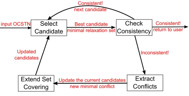
3-2 John’s trip modeled as an Optimal Conditional Simple Temporal Network 65 3-3 The program flow of Conflict-directed Relaxation Enumeration . . . . 73

3-4 Cascaded inverters with different rates of failure . . . 75

3-5 Duality between minimal conflicts and minimal relaxation sets . . . . 78

3-7 A minimal conflict in John’s trip plan . . . 82

3-8 Another minimal conflict in John’s trip plan . . . 82

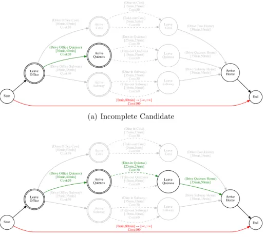
3-9 Examples of expanding incomplete candidates . . . 88

3-10 A real valued objective function for John’s trip plan TPN . . . 90

3-11 The real valued cost for a minimal relaxation set . . . 91

3-12 Convert a simple temporal constraint to arcs in a distance graph . . . 93

3-13 A negative cycle in a distance graph . . . 94

3-14 John’s trip without the temporal goal of duration . . . 96

3-15 Examples of splitting negative cycles with a common vertex . . . 99

3-16 An OCSTN with a conflict . . . 99

4-1 Examples of continuous relaxations to a temporal constraint . . . 105

4-2 Examples of semi-convex preference functions (a)-(c) and non-semi-convex functions (d)-(e) . . . 109

4-3 An inconsistent OCSTN . . . 110

4-4 Cost functions over constraints TimeConstraint and Dinner at Cosi110 4-5 Discrete temporal relaxations for John’s trip . . . 111

4-6 Continuous temporal relaxations for John’s trip . . . 112

4-7 Cost after continuously relaxing TimeConstraint and (dine-in Cosi) . 113 4-8 Examples of discrete relaxations . . . 113

4-9 Examples of continuous relaxations . . . 114

4-10 The program flow of Continuous BCDR . . . 118

4-11 Two steps in the generation of constituent relaxations . . . 123

4-12 Examples of continuous temporal relaxations . . . 135

4-13 Continuous preference functions over the constraints . . . 136

5-1 20-constraint test case: 2 decisions with 10 constraints . . . 142

5-2 20-constraint test case: 10 decisions with 2 constraints . . . 142

5-3 20-constraint test case: 80% over-constrained . . . 144

5-4 Runtime on randomly generated temporal problems with different num-bers of constraints . . . 147

5-5 Runtime of Uhura (using BCDR) on temporal problems with different

numbers of choices . . . 148

5-6 Runtime of Uhura (using BCDR) on temporal problems with different

over-constrained levels . . . 150

5-7 Runtime of continuous BCDR on relaxation tests . . . 152

List of Tables

5.1 Specification of benchmark Optimal Conditional Simple Temporal

Net-works . . . 143

Chapter 1

Introduction

As the performance of temporal planning algorithms improves over time, they have been incorporated into many planning and scheduling applications. However, a plan that can satisfy all of the user goals does not always exist. For example, a Mars rover may encounter an unexpected battery failure, leaving little time to complete its exploration task. Usually, planners will signal the user that a feasible plan that can satisfy all the goals cannot be found. However, it is not enough for the system to just signal a failure. When the complexity of the problem and plan increase, it becomes extremely difficult for humans to identify the resolutions. Therefore, the autonomous system or decision aid should explain the situation and propose alternative plans so that the engaged human operator can find a more informed resolution without too much effort. Specifically, the decision tool should offer key insights into the cause of failure and preferred plan repair options to the operator. For example, in the context of a Mars rover with a failed battery, we would expect the system to tell us which goals need to be dropped in order to guarantee a safe return to the base

This thesis develops Uhura, a temporal plan relaxation algorithm and system that addresses these issues. Uhura takes a mixed initiative approach that generates

preferred minimal relaxations to over-subscribed temporal planning problems. It

works with the human collaboratively towards the diagnoses of faulty plans. Uhura has three significant features compared to previous approaches: quick response, simple interaction and small perturbations. To support these features, we developed three

new methods in this thesis:

• First, Uhura minimizes the perturbation of relaxations to the original planning problem by continuously relaxing its goals specified by temporal constraints, which preserves all the plan elements in the output relaxed problem. For ex-ample, instead of about the mission completely, the rover informs the operator about an extended completion time.

• Second, Uhura resolves over-subscribed temporal planning problems through a conflict-directed diagnostic process, making it very efficient for relaxing large scale applications. A conflict can be viewed as a summary of cause of failure. In the Mars rover scenario, there is a conflict between the mission goals and limited battery power that makes the problem infeasible. To resolve a conflict, one must relax at least one goal in it, such as extending the mission completion time. A valid relaxation restores the feasibility of a planning problem by resolving all its conflicts.

• Third, Uhura only enumerates minimal relaxations, a compact representation of relaxations to over-subscribed planning problems. It reduces the size of results by orders of magnitude and significantly improves the run-time performance. For example, the rover will only asks the operator for either an extended mission time or a reduced set of goals, but not both.

We first provide an overview of the features and desired behaviors of Uhura through the trip planning problem of a Personal Transportation System, which is a form of robotic air taxi, in Section 1.1. Section 1.2 presents the current approaches to each claim and the technical challenges of their implementations. Finally, we describes the structure of the thesis in Section 1.3.

1.1

Motivation: Over-subscribed Problems are

Ev-erywhere

Nowadays, autonomous planning systems have been widely used in people’s lives, especially in the fields of transportation and manufacturing. They have been used to generate the routes and schedules of flights, trains, buses and cars, and for generating work plans. Modern planning algorithms have demonstrated superior capabilities, especially for large scale problems that are beyond human decision making capabil-ities. For example, a planning and scheduling algorithm, O-Plan, has been used to generate production plans for Hitachi [6]. Their implementations have significantly reduced the workload of human operators and for optimizing operation efficiency .

A significant open challenge is to decide what to do when the situation is over-subscribed. For example, a Mars rover encounters an unexpected battery failure, leaving insufficient power for the rest of its mission. If a problem is over-subscribed, that is, no plan exists that can satisfy all the goals and requirements imposed by either human operators or the environment, these planners cannot help resolve such a problem. In this thesis, we introduce a novel approach to the over-subscribed problem based on the metaphor of collaborative diagnosis. Handling over subscription through collaborative diagnosis is based on two central claims:

• Handling over subscription is inherently a collaborative process. The operator knows the relative importance of different goals. It is unreasonable to expect that the operator will have presented this preference information to the planner a priori, and hence the planner will be able to decide the appropriate relaxation alone. Conversely, the human will need the planning tool to help explore the space of possible goal relaxations. The planner will have expertise and brute computational power that is better suited to this task.

• For the human to make informed decisions, the planner should be able to sum-marize the results of its reasoning processes to the human decision maker, as it pertains to the decisions that the human needs to make. This includes

diag-nostic information, such as why a set of goals cannot be feasibly achieved, and why a proposed relaxation addresses each of these identified concerns.

• We claim that over subscription can often be addressed with minimal disruption by relaxing constraints partially. We refer to this as continuous relaxation. The motivation is that the users usually want to minimize the perturbation to their goals and constraints made by the resolutions. Resolving over-subscribed problems by completely suspending user goals is unnecessary in most situations.

A better way would be to adjust the user goals accordingly. For example,

a student realizes that he cannot complete his problem set on time due to an approaching exam. Instead of giving up the exam or the problem set, he chooses to ask for an extension for his problem set, thus preserves his goals to the maximum.

The vision of this thesis is to provide an autonomous system that can detect the cause of failures in over-subscribed temporal plans, engage the human operators and provide suggestions for the repairs. The following three features are necessary for resolving over-subscribed problems: quick response, simple interaction, and small perturbation.

Quick response

The algorithm implemented in the diagnosis system should be efficient. Usu-ally, people would expect an instant resolution coming out from the system if their plans are known to be broken, say within 1 to 2 seconds. Efficient algo-rithms help to implement quick response, and hence make the diagnosis process convenient for the users.

Simple interaction

The resolutions generated by the system must be compact and concise so that they can be communicated to the users easily. For example, in the Mars rover scenario, the operator would be more interested in the few goals that have to be dropped, not the ones that remain achievable. If multiple resolutions are

available, the system should be able to select the leading candidates preferred by the operator. Otherwise, it may take a long time for the operator to look through the long list of possible resolutions to a large scale problem. Moreover, the preference models should be easy to construct and evaluate.

Small perturbation

The resolutions generated by the system must minimize the perturbations made to the original problem. In other words, if an over-subscribed temporal planning problem can be resolved by removing one goal, the system should not suggest the user to remove more than that.

Collaborative diagnosis supports the first two features. It enables autonomous systems to provide quick response and simple user interaction. The extension to continuous relaxation enables user goals to be preserved to the maximum degree possible in the resolution to over-subscribed problems. We present a scenario in the following subsection to demonstrate the challenges and our approaches to the solution.

1.1.1

Planning a Trip Home Using the Personal

Transporta-tion System

Throughout this thesis, discussion will center around the example of the Personal Transportation System, a joint project between the Model-based Embedded and Robotic System group at MIT, the Boeing Company and the Center for the Study of Language and Information at Stanford University. This project aims at demon-strating the concept of an autonomous Personal Air Vehicle (PAV, Figure 1-1), and possibly on a vehicle similar in spirit to the Transition (Figure 1-2), in which the passenger interacts with the vehicle in the same manner that they interact with a taxi driver. To interact with a PAV, the passenger describes his/her goals and con-straints in English. The autonomous system on-board the PAV checks the map and weather conditions, generates a safe plan and flies the vehicle to the destination. If there is a change in the weather condition or the destination airport is closed due

to flow control, the system can automatically adjust the original plan to achieve the passenger’s goals.

The Temporal Plan Relaxation system, Uhura1_{, is developed as he part of the}

project that supports collaborative diagnosis of over-constrained temporal plans. The state and temporal goals provided by the passenger may not be consistent for all times. Both the lack of knowledge about the vehicle and changes in environment constraints may cause inconsistency between the user’s goals. However, the scale and complexity of the temporal plans are usually very large, making it difficult for a human being to detect the cause of failures and to find resolutions. Uhura is developed to work with the users collaboratively to resolve problems through schedule relaxations, similar to a travel agent. Uhura will propose alternatives to the user when an over-subscribed problem is identified, and negotiate with the user until an agreement is reached.

Figure 1-1: The Personal Air Vehicle simulated using X-Plane

Suppose that the passenger, John, just finished his work in the office and needs to be home in 60 minutes for a friend’s birthday party. On his way back home, he would like to have dinner at a sandwich restaurant. The restaurant options he has are Cosi, Quiznos and Subway. Each restaurant has different waiting and dinner times, and the driving distances required by them are different as well. With the integration of a natural language dialog system developed by CSLI Stanford University [38], Uhura

Figure 1-2: The Transition flying car (Courtesy Terrafugia)

can interact with the user and capture all the goals through a simple conversation:

John: This is John.

PAV: Authorization Confirmed.

John: I want to go home in 60 minutes.

PAV: OK.

John: I want to stop at a sandwich restaurant for dinner.

PAV: OK. I found three sandwich restaurants on your way back: Cosi,

Quiznos and Subway. Do you want to dine-in or take-out?

John: Both are fine.

PAV: Ok...

PAV: I cannot find a plan for you.

PAV: Your goal of arriving home in 60 minutes can not be achieved.

There appear to be three good options, given your preferences. First, can you relax your goal to 85 mins?

John: No.

PAV: Then can you go home directly without having dinner?

John: No.

say 40 mph?

John: Ok, I think I can accept it this time.

PAV: OK, I have found a feasible plan for you.

John: Thank you PAV.

First, the planning algorithm of Uhura detects that no plan exists that can sat-isfy all of John’s goals. Uhura then identifies the cause of failure: the temporal goal proposed by John (60 minutes) is too tight to complete all the tasks. Based on this conflict, collaborative diagnosis starts enumerating resolutions and engages John to negotiate for an alternative plan. For example, the PAV presents John an option that changes the trip duration. John rejects its proposal and Uhura continues the enumeration and looks for the next schedule relaxation that resolves the prob-lem. Collaborative diagnosis continues proposing new resolutions until it reaches an agreement with John.

To make the collaborative process efficient, that is, reaching an agreement with the user as soon as possible, user preference models are used in the collaborative diagnosis algorithm. The end goal is for the user to select a relaxation that best meets the user’s needs. Typically the space of feasible options is too large for the human to consider; instead the human would like to be presented with few good options. To do this the collaborative diagnostic algorithm needs to know the passengers’ preferences. To address this requirement, Uhura generates a list of preferable repair options based on a metric cost function that encodes the passengers’ preference over restaurant choices and the relaxations of schedule constraints. The user-preferred relaxations will be generated and presented first, hence shorten the negotiation process.

Second, the continuous relaxation algorithm post-processes the resolutions gen-erated by the collaborative diagnosis algorithm and tries to preserve the user goals as much as possible. For example, the PAV notices that removing the duration con-straint (60 minutes) can resolve the conflict in John’s plan. Continuous relaxation then computes the minimal amount of adjustment to this constraint that is sufficient to resolve John’s over-subscribed problem, without completely suspending this

dura-tion constraint. In this case, the constraint is relaxed from 60 minutes to 85 minutes, which is the resolution with the minimal perturbation.

In addition to the Personal Transportation System, Uhura has also been tested within many other applications, including a robotic driving assistant system, AIDA (for Affective Intelligent Driving Agent), that provides suggestions to help drivers resolve timing conflicts in their trip plans (Figure 1-3).

(a) The AIDA Robot. (b) User interface of AIDA.

1.2

Related Work and Challenges

We outlined three goals for Uhura: quick response, simple interaction, and small perturbation, in Section 1.2. To address these goals, we introduce two innovative ap-proaches to resolve over-subscribed temporal planning problems: Best-first Conflict-Directed Relaxation (BCDR) and continuous relaxation. In this section we present the technical challenges of implementing the approaches to satisfy these goals, and related work in the literature.

1.2.1

The Search Space is Enormous

Planning problems are generally very hard to solve due to the large numbers of possible states and activities, and their possible combinations. The same problem exists during the resolution of over-subscribed temporal planning problems. The number of possible resolutions is exponential: every state and temporal goal in the plan may be relaxed. For example, the temporal planning problem of booking a trip from Boston to Detroit has around 30 planning steps, and the number of possible

resolutions can be as large as 1010.

This enormous search space imposes a huge challenge to resolving over-subscribed temporal problems efficiently and to providing a quick response to the users. In fact, the problem of finding all the resolutions to an over-subscribed temporal planning problem is NP-Complete [29], assuming that a polynomial algorithm exists that can check if a temporal plan is executable.

Many techniques, especially the techniques developed to solve constraint satisfac-tion problems, have been implemented to speed up the search for resolusatisfac-tions, includ-ing standard and domain specific ones, such as forward checkinclud-ing, conflict-directed back jumping, Dualize & Advance [4], removal of subsumed variables [27] and seman-tic branching [3] (the last two techniques only apply to temporal problems). Temporal planning problems can be encoded using CSP formulations, hence enable the use of these techniques. One other approach is to give up the requirements on the com-pleteness of the results and use a local search algorithm, like [5]. This approximate

approach usually runs much faster than the systematic methods, however, cannot guarantee the optimality or completeness of the results.

1.2.2

The Number of Resolutions is Far Beyond Human

Rea-soning Capability

The large numbers of results is also an issue for the users: facing thousands or even millions of resolutions, it is difficult for a human to select the correct one from them. This imposes a big challenge to resolving a problem through simple and efficient human machineinteraction. The autonomous system must be able to filter out un-necessary and less-preferred resolutions and only present a few preferred ones to the user, in order to let the user make an informed decision. In [29], an approach is presented to reduce the amount of resolutions generated by generating representa-tive plan relaxations. It is based on the notion of representarepresenta-tive set, in which all resolutions generated cannot be dominated by any other resolutions in the set.

In addition, most approaches choose to implement preference models to help re-solve this issue. In [30], a real-valued cost function is associated with all the plan goals in order to evaluate and prioritize the resolutions generated by the algorithm. However, its preference function is restricted to discrete domain variables, in which constraints are either preserved or suspended. For continuously relaxed constraints, the preference function is more complex, since the relaxation has infinite numbers of states. For example, John’s preference over the relaxation of duration constraint may depend on its extent. If the constraint is slightly relaxed, the relaxation is indifferent for John. On the other hand, if the constraint is relaxed by 100%, John may give up the whole trip due to his limited amount of time.

1.2.3

Perturbations to the User Goals Must Be Minimized

As stated before, the user would like to preserve his/her goals to the maximum, if possible, in the resolutions to an over-subscribed temporal planning problem. This challenge corresponds to the third requirement: small perturbation. As a valid

reso-lution, it must relax some of the user’s goals on states and temporal constraints, like delaying the arrival time or removing way points from the trip. The perturbation to the user’s goals is unavoidable.

Most of the previous work takes an all-or-nothing approach, in which user goals are suspended in order to resolve the over-subscription problem [16, 5, 31]. However, suspending goals can perturb a problem a significant amount, and is often unneces-sary. For example, in John’s trip, it would be unnecessary if the PAV asks him to remove his constraint on trip duration, since slightly relaxing the duration is enough to make his plan executable.

In [30], temporal relaxation is divided into several levels. For example, John’s constraint on trip duration may be relaxed to 70, 80 or 90 minutes, depending on the over-subscription and John’s preference. This approach preserves more plan elements than complete constraint relaxation, however, the quality of its resolutions highly depends on the discretization of the domain of users’ goals.

1.3

Thesis Layout

This thesis presents two innovations that address the three challenges. First, we present the collaborative diagnosis algorithm, Best-first Conflict-directed Relaxation (BCDR), used in Uhura that enumerates minimal temporal relaxations and nego-tiates alternative options to over-subscribed temporal planning problems with the user. Through the implementations of conflict-directed best-first enumeration and minimal temporal relaxations, BCDR addresses the second and third requirements we presented in Section 1.1: simple interaction and small perturbation. It improves the efficiency of enumerating relaxation by two orders of magnitude compared to previous approaches. In addition, BCDR generates minimal relaxations, a compact representation of all relaxations to over-constrained temporal planning problems. The use of minimal relaxations significantly reduces the size of the search space and the results.

We present the algorithm in two steps: first we present a simpler version of BCDR that generates discrete relaxations. Then we present the continuous version of BCDR that maximizes the preservation of user goals. Unlike discrete relaxations to tem-poral constraints, continuous relaxations do not suspend any temtem-poral constraint. Instead, it adjusts temporal constraints continuously until an executable plan can be generated. It can find the ’minimal’ relaxation that is necessary for resolving over-subscribed problems, hence minimizes the perturbation to the users’ goals.

In this thesis, we relax over-subscribed temporal planning problems. We achieve this by encoding them as inconsistent conditional temporal constraint networks, and by relaxing these constraints continuously. We demonstrate that the relaxation to the schedule of a planning problem is in fact equivalent to relaxing constraints in its equivalent temporal constraint problem, since each schedule constraint in the planning problem can be mapped to a unique temporal constraint in the constraint problem. BCDR is developed as a general constraint programming algorithm that can resolve any inconsistent conditional CSPs with discrete and continuous variables. It takes in an inconsistent problem and resolve all of its conflicts, by relaxing one or more of its

constraints.

In Chapter 2, we defines the related concepts used in this thesis, including the description of user goals (Qualitative State Plans), solutions (Temporal Planning Networks), cause of failure (Conflicts) and resolutions (Temporal Relaxations). In Chapter 3, we present the Best-first Conflict-directed Relaxation algorithm that enu-merates minimal discrete relaxations to over-subscribed temporal problems. In Chap-ter 4, we describe the continuous version of BCDR and its integration with Uhura. In Chapter 5, we present the experimental results of BCDR on various benchmark prob-lems. Finally, in Chapter 6 we summarize our work and discuss possible extensions to Uhura for future work.

Chapter 2

The Problem of Continuous Plan

Relaxation

As discussed in Chapter 1, this thesis presents a general method for collaborative plan relaxation through diagnosis, and a more general, underlying method for contin-uously relaxing constraints on both discrete and real-valued variables. This method is demonstrated in the context of user interaction with a robotic air taxi. This chapter develops the problem statement, defines key supporting concepts and demonstrates each in the context of the Personal Transportation System scenario from Chapter 1. As humans we are often inclined to do too much, and as a result discover that there is no way to achieve all of our goals. When this occurs, we consciously or unconsciously relax some of those goals until what remains is do able. Our problem is to provide an algorithm that aids a user in systematically exploring the space of goal relaxations. To turn this into a formal problem statement, we need to make precise the terms: goal, executable, relaxation and preference.

In our approach we view both goals and their executions as a form of temporal plan comprised of a set of activities to perform, such as go to the store, and constraints on their timing, such as depart in the next 30 minutes, and return within an hour. The difference between the plans used to describe goals and executions is their specificity. Goal plans provide general guidelines that are important to the user, such as have groceries in a hour, while an executable plan specifies concrete activities that we know

how to perform, such as turn in the car engine.

Given the central role of plans in goal relaxation, we begin by making precise these different concepts of plan and their execution. In a general planning problem, the goal is to generate a set of actions that can achieve all desired goals given a description of the environment, allowed actions and initial state. Usually, a planning problem involves three basic elements: A Planning Domain, A set of Goals and A Plan.

• A Planning Domain specifies a set of legal states and actions allowed in the planning problem.

• The initial states specify the status of the agents at time t=0.

• The Goal of a planning problem is a set of desired states at different times. • A Plan is the solution to a planning problem, which involves a set of legal

actions that, starting in the initial state, generate a set of states at different times that entails the Goal.

In this thesis, we use Qualitative State Plans (QSP) [24] to describe time evolved goal states given by the user. A QSP uses episodes and temporal constraints to specify the user goals, where episodes are constraints on state trajectories, over a bounded interval of time. An episode is our general term for an activity, whether it is abstract or concrete. We assume that an algorithmic temporal planner is used that takes a planning domain, initial states and a QSP as input, and returns a plan or a set of plans if one exists, or a signal indicating that no plan exists.

We use Executable Temporal Plans (Temporal Plans for short) to represent the solution to a planning problem. A temporal plan contains a set of activities, which represent action sequences that can generate state trajectories to satisfy the goals specified in QSPs. We say that a plan is complete if it logically entails all goals in the QSP, and consistent if the plan itself is logically consistent, that is, all the preconditions and maintenance conditions of all activities are satisfied. A planning problem is feasible if a complete and consistent plan exists for it. In addition, we use

Temporal Plan Networks [22] to encode a candidate set of temporal plans that may be used to satisfy a QSP.

A planning problem is infeasible if no consistent temporal plan that entails all goals in the QSP exists. That is, no plan can satisfy all the goals described in the QSP. The cause of failure is the conflicts between the goals and planning domains, that is, the allowed actions and states in the plan are insufficient for satisfying the goals. For an inconsistent planning problem, there is either no complete plan that entails the QSP, or all complete plans that entail the QSP are inconsistent.

To resolve an infeasible temporal planning problem, we need to remove or change some of the goals in the QSP so that a complete and consistent plan can be generated. In this thesis, we focus on restoring the consistency of an inconsistent temporal plan by modifying some goals in the QSP. Such a modification is called a relaxation to a QSP, and can be applied to either goals on states that are specified by episodes, or goals on temporal relations that are specified by temporal constraints. More specifi-cally, we focus in this thesis on schedule relaxations, which relax the users’ temporal constraints, in this thesis.

In Section 2.1, we present the definition of the goal specifications in temporal plan-ning problems using QSPs. In Section 2.2, we describe the solutions using temporal plans and TPNs. Then we discuss the causes of infeasible temporal planning prob-lems in Section 2.3. Finally, in Section 2.4, we present relaxations as the resolutions to infeasible temporal planning problems.

2.1

Modeling User Goals using Qualitative State

Plans

This section introduces a representation that captures the users’ desired goals in a planning problem. In the PTS scenario, the passenger, John, propose a set of goals he would like to achieve throughout his trip. These include his requirements on time, such as Arrive home in 80 minutes, and requirements on the locations, like Dinner at a sandwich restaurant. In general, all the goals and requirements of a user can be described explicitly using a set of time evolved states and temporal constraints. The desired evolution of goal states can be represented as a Qualitative State Plan (QSP):

Definition 1. A Qualitative State Plan (QSP) is a tuple < E , E PS, T C, estart, eend >>

where:

• E is a set of events. Each event e ∈ E can be assigned a non-negative real value, and denotes a distinguished point in time.

• EPS is a set of episodes. Each episode specifies one or more allowed state trajectories between a starting and an ending event.. They are used to represent

the state constraints. An episode is a tuple < eS, eE, l, u, SC > where eS and

eE in E are the start and end events of possible state trajectories, l and u are

lower and upper bounds on the time duration of the episode and SC is a set of state constraints that must be true over the duration of the episode. In this thesis, the set of state constraints SC is represented by a conjunction of PDDL predicates.

• T C is a set of simple temporal constraints between events E. It is used to repre-sent the temporal constraints in the QSP. A simple temporal constraint [12] is

a tuple < eS, eE, LB, U B > where: eS and eE in E are the start and end events

of the temporal constraint. LB and U B represent the lower and upper bounds

of the duration between events eS and eE, where LB ∈ R∪−∞, UB ∈ R∪+∞

• estart and eend ∈ E are two distinct events that represents the first and last events in the QSP.

For example, the QSP of John’s trip is summarized in (Figure 2-1).

Start Leave Office (at Home) End [0min,80min] Arrive Food Service Leave Food Service (have sandwich)

[5min,35min] ArriveHome (at Home)

Figure 2-1: The Qualitative State Plan of John’s trip

The events in the graph are represented by circles, and episodes and temporal constraints are represented by arrows. The QSP is a goal specification, comprised of two types of constraints: state constraints and temporal constraints. They are represented by episodes and simple temporal constraints. In (Figure 2-1), the episodes are represented by blue arrows with a label indicating the state constraint. A state constraint is a conjunction of propositions, where each proposition is a predicate applied to one or more variables and constraints, such as location and temperature. There are three types of state constraints that are allowed:

• Constraints on the states of the agents in a QSP, like locations, temperature and velocity.

• Instantiations of primitive PDDL operators, like movements and deformation. • A program which can be expanded to a QSP.

For example, (Figure 2-2) shows an example of a QSP episode that constrains the location, which represents the user’s requirement of not staying at the office.

e_S (not (at office)) e_E

In John’s QSP, there are three episodes, specifying his three state constraints: the trip starts from his home (at John home), needs to include a sandwich place for dinner (have sandwich John) and finally returns home (at John home).

In addition, there are two temporal constraints: the dinner should last between 5 and 35 minutes, and the trip duration should be less than 80 minutes. These specify the relation that John would like to achieve between his state constraints. Temporal constraints in a QSP are described by Simple Temporal Constraints.

e

[LB,UB]

e

Figure 2-3: A Simple Temporal Constraint

A simple temporal constraint is represented by labeled red arrows in the graph

(Figure 2-3). The constraint arrow starts from the start event (eS) and points to the

end event (eE). The lower bound of a simple temporal constraint is unconstrained

if it is set to LB = −∞. Similarly, its upper bound is unconstrained if U B = +∞. There are several special forms of simple temporal constraints that are commonly used while describing real world scenarios (Figure 2-4):

e

[-infinity,0]

e

(a) eE no later than eS

e

[0,+infinity]

e

(b) eE no earlier than eS

e_S [6min,+infinity] e_E

(c) eE at least 6 mins later than eS

e_S [-infinity,+infinity] e_E

(d) Constraint suspended

2.2

Modeling Solutions to User Goals as Temporal

Plan Networks (TPNs)

This section reviews the representation of solutions to a temporal planning problem. As mentioned in the intro section, the solution to a planning problem is a temporal plan, which is a set of activities that satisfies all the state and temporal constraints in a QSP. We present two key concepts that define a valid plan in this section: Completeness and Consistency.

2.2.1

Encoding One Solution using Temporal Plans

A Temporal Plan is a formalism that specifies a set of activities that can satisfy all state and temporal constraints in a QSP, which is a specification of users’ goals. Its form is similar to that of QSPs, but the episodes in a QSP are restricted to activities. Formally, a Temporal Plan is defined as:

Definition 2. A Temporal Plan is a tuple < E , ACT , T C, estart, eend > where:

• E is a set of events. Each event e ∈ E is assigned a non-negative real value, and denotes a specific instant in time. This is the same concept as event in QSPs.

• ACT is a set of activities between events. It is a specialization of an episode. An activity is an episode in which its state constraint is expressed by an operator

instantiation. An activity is a tuple < eS, eE, l, u, act >. Each activity has a

start event eS, an end event eE, a minimal duration l, a maximum duration

u and an action act. In this thesis, act is an action that represents a state transition, through its preconditions and its effect. More generally, an activity represents a state trajectory over its duration. The duration of the activity will be restricted by the temporal bounds, [l,u]. If u > l, this activity is a partial operator instantiation since the duration of this activity is flexible. Otherwise this activity is a full operator instantiation.

• T C is a set of simple temporal constraints. Like QSPs, simple temporal con-straints in temporal plans specify the allowed durations between events. In ad-dition, T C and ACT entail the temporal constraints in the QSP.

• estart and eend∈ E are two distinct events that represent the first and last events

in the temporal plan. We assume that the time assigned to estart, testart is

al-ways 0. estart and eend are always connected by activities or simple temporal

constraints, or a combination of both.

Temporal plans share the same structure as qualitative state plans. The difference is that a temporal plan contains a set of activities, instead of episodes, that can satisfy the required state trajectories stated in the QSP. In other words, a QSP contains a set of goals and a temporal plan contains activities that will achieve those goals. For example, if a state constraint in a QSP imposes a transition between two locations, (at office) and (at home), then an activity, (Drive office home), may be found in the temporal plan that satisfies this constraint.

Each activity in a temporal plan implies a fully or partially instantiated state trajectory that entails some of the episodes in QSPs. This is because the start time of each activity may be fully specified or flexible, depending on the temporal constraints. If the activity has a firm start time and duration, then it will generate a set of fully

instantiated state trajectories. The temporal constraints in a plan represent the

temporal relations between activities, and entail the temporal constraints in its QSP. A temporal plan is a feasible solution to a planning problem if it is Complete and Consistent. A Complete temporal plan logically entails all the goals, which are specified by state and temporal constraints in the QSP.

Definition 3. [Completeness of Temporal Plans] A temporal plan P for a QSP Q, is complete if the activities and temporal constraints in P entail Q, P |= Q. In other words, all the state and temporal constraints in Q can be satisfied by P.

A temporal plan is state complete if all the state constraints E PS in Q are entailed by all activities and temporal constraints in P.

A temporal plan is temporally complete if all the temporal constraints T C in Q, are entailed by all activities and temporal constraints in P.

A temporal plan is complete if it is both spatially and temporally complete.

On the other hand, even though a complete plan achieves all the goals specified in the QSP, it may not be a valid solution due to its inconsistency. The consistency of a temporal plan is about the consistency of the elements in it. It is necessary in order for the plan to be executed.

Definition 4. [Consistency of Temporal Plans] A temporal plan P is consistent if the activities ACT and temporal constraints T C in P are logically consistent. In other words, no logical contradiction can be derived from P.

A temporal plan is spatially consistent if all the activities ACT ∈ P, are con-sistent. That is, two actions do not threaten each other. This correspond is enforced through mutual exclusions.

A temporal plan is temporally consistent if all the temporal constraints T C ∈ P, are consistent and are satisfied by the durations of ACT .

The consistency of a temporal plan indicates whether it can be correctly executed. In most cases, the state and temporal consistency of a plan are coupled, since the preconditions and maintenance conditions of an activity may hold only during a certain period of time. For example, assume that drinking a bottle of soda requires

two activities: Opening the bottle and Drinking. Then a temporal plan of these

activities is spatially consistent if and only if the temporal constraints allow Opening the bottle to be executed prior to Drinking. In [25], a method is presented to check the spatial consistency of activities with flexibility in execution time. In this thesis, we assume that a set of temporal constraints has been introduced by the planner to guarantee that the sequence of activities satisfy the pre- and maintenance conditions of all activities at the times required.

In order to execute a temporal plan correctly, the activities of a temporal plan must be executed at proper times that satisfy all temporal constraints in the plan. The dispatch time of an activity is the same as the time assigned to its start event,

and the duration of the activity is the difference between the time assigned to its start and end events. The time that activities are executed is specified by a schedule for the temporal plan.

Definition 5. (Schedule for a Temporal Plan) A consistent schedule T for a temporal plan P is a set of time assignments to all its events, E , such that all the temporal constraints and activity durations in P are satisfied. Each event, e ∈ E , is

assigned a time point te. For each temporal constraint and activity duration in P, the

time assignments to its start and end events satisfies: T CLB ≤ tend− tstart ≤ T CU B.

T CLB and T CU B are the lower and upper bound of an activity duration or temporal

constraint.

For example, one temporal plan that can satisfy John’s goals is shown in (Figure 2-5). He may drive to Quiznos for dinner after he leaves his office. There are three ac-tivities in this plan: ’Drive from Office to Quiznos’, ’Take-out sandwich from Quiznos’ and ’Drive from Quiznos to Home’, represented by green arrows in the graph. The duration of each activity is different: ’Take-out Quiznos’ is fully instantiated and the duration is fixed to 10 minutes, while the other activities are partially instantiated. Driving from office to Quiznos may take any time between 30 and 40 minutes. The definition of entailment between temporal plans and QSPs is presented in [25].

There is a temporal constraint that specifies the overall time requirement of the QSP: [0min, 80min]. It connects the first and last events in the temporal plan and restricts the duration of the whole trip. Similar to QSPs, temporal constraints are represented by red arrows in temporal plan graphs.

Start Leave Office t=0min End [0min,80min] Arrive Quiznos t=30min

(Drive Office Quiznos)

[30min,40min] _QuiznosLeave

t=40min

(Take-out Quiznos)

[10min,10min] Arrive_Home

t=75min

(Drive Quiznos Home) [35min,50min]

Figure 2-5: A schedule for a temporal plan

The time marked on each event shows a schedule for John’s trip plan back home: • Leave home right now (0 minute).

• Arrive at Quiznos 30 minutes from start.

• Ask for take-out and leave Quiznos 40 minutes from start. • Arrive home 75 minutes from start.

It can be seen from the graph that all the temporal constraints and activity durations are satisfied by this consistent schedule: John spends exactly 10 minutes having dinner at Quiznos and the time assigned to two driving activities falls into the allowed durations. For any temporal plan, we can use the existence of a schedule to check its temporal consistency.

Definition 6. [Temporally Consistent Plans] A temporal plan P is temporally con-sistent if there exists at least one concon-sistent schedule, T to P. That is, there is at least one set of time assignments to all events, E in P such that all the temporal constraints, including activity durations, are satisfied.

For example, the temporal plan in (Figure 2-5) is temporally consistent, since it has a consistent schedule that satisfies all temporal constraints. However, if John reduces his expected arrival time from 80 minutes to 60 minutes (Figure 2-6), then no consistent schedule can be found. Such a temporal plan is not consistent, and more specifically, is defined as an over-constrained temporal plan.

Start Leave Office End [0min,60min] Arrive Quiznos

(Drive Office Quiznos)

[30min,40min] Leave

Quiznos

(Take-out Quiznos)

[10min,10min] _Arrive

Home

(Drive Quiznos Home) [35min,50min]

Figure 2-6: An over-constrained temporal plan

Definition 7. [Over-constrained Temporal Plan] A temporal plan P is over-constrained if P does not have a consistent schedule. In other words, it is complete with regards to a QSP, but there are no time assignments to the events in P such that all its temporal constraints, including activity durations, can be satisfied.

2.2.2

Encoding Multiple Contingent Solutions using

Tempo-ral Plan Networks

For a QSP, there might be more than one plan that is complete and consistent: several temporal plans may be found to satisfy the goals in one QSP. Usually, this is a result of two reasons:

• The goal specification in a QSP may be instantiated in different ways. For example, in John’s scenario, the QSP only specifies his requirement of (Having Dinner at a Sandwich Place), but does not indicate which restaurant to go to. This episode can be instantiated with any sandwich restaurant that is on his way back home, such as ’Dinner at Subway’. Therefore, a QSP may represent multiple consistent executions if not all episodes in it are fully grounded. • There may be multiple ways to satisfy one state constraint. For example, John

may ask the planner to find a plan back home from his office. The planner identifies several different ways to commute: (Drive Office Home), (Taxi Office Home) and (Bike Office Home). A temporal plan can be generated based on each mode of commuting, hence multiple plans may be available to solve John’s problem.

To represent a set of candidate plans that satisfy a QSP, we use the concept of Temporal Plan Networks (TPN), a compact representation of multiple temporal plans introduced by [22].

Definition 8. A Temporal Plan Network (TPN) is a tuple < E , SP, T C, DE , estart, eend >

where:

• E is a set of conditional events. Each event e ∈ E is a plan element that can be assigned to a specific point in time. A conditional event, e, may belong to different sub plans. e will only occur and be scheduled if any of those sub-plans are selected and executed.

• SP is a set of sub-plans. Each sub-plan is either a temporal plan, or a TPN.

The start and end events of a sub-plan belongs to E , that is, es and ee ∈ E.

• T C is a set of simple temporal constraints. Like temporal plans, simple temporal constraints in TPNs specify the allowed temporal durations between events, and entail the temporal constraints of the QSPs.

• DE is a set of decision events in the TPN, and is a subset of E. A decision event, de, is an event followed by a subset of sub-plans: only one of them can be selected at a time. Its domain, DSP, is the set of all sub plans whose start event is de.

• estart and eend∈ E are two distinct events that represent the first and last events

in the TPN. We assume that the time assigned to estart, testart is always 0. Both

events are always connected by sub plans or simple temporal constraints, or a combination of both.

A TPN is a nested set of non-deterministic choices between alternative sub plans [23]. It is a compact representation of multiple temporal plans using choices: the activation of sub plans depends on the choices made to the decision events. In this thesis, we use TPNs to represent a combination of a (possibly incomplete) set of candidate plans that may satisfy the users’ goals in a planning problem.

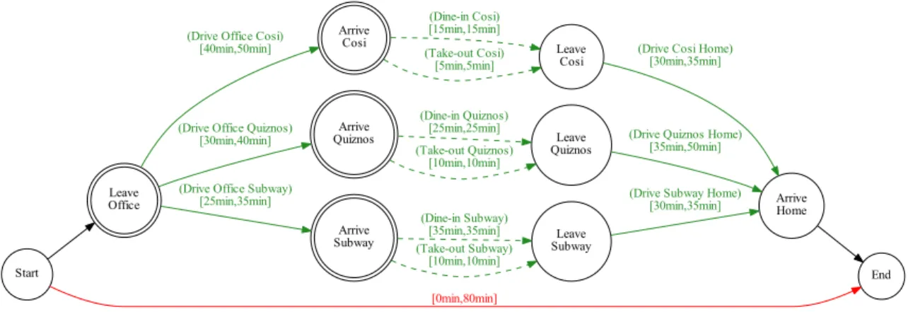
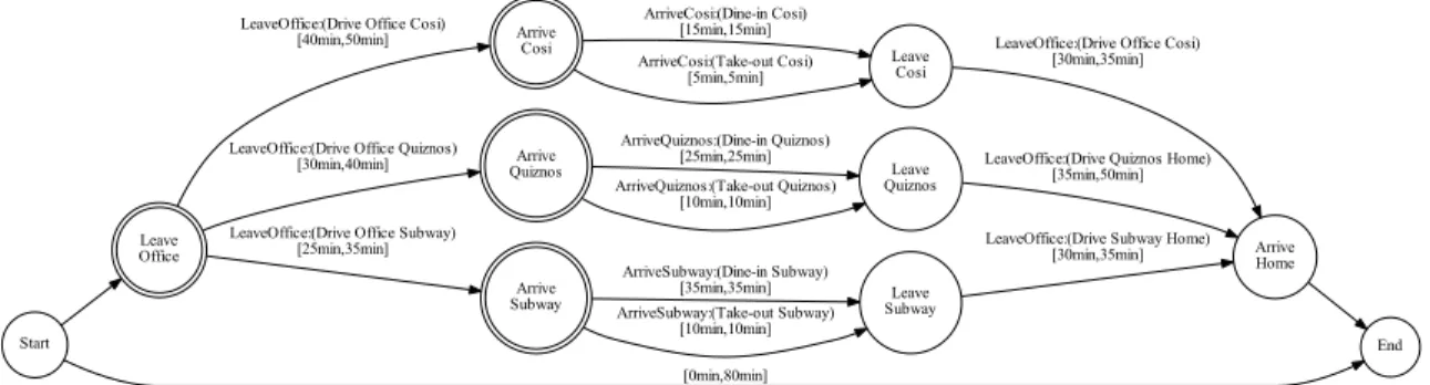
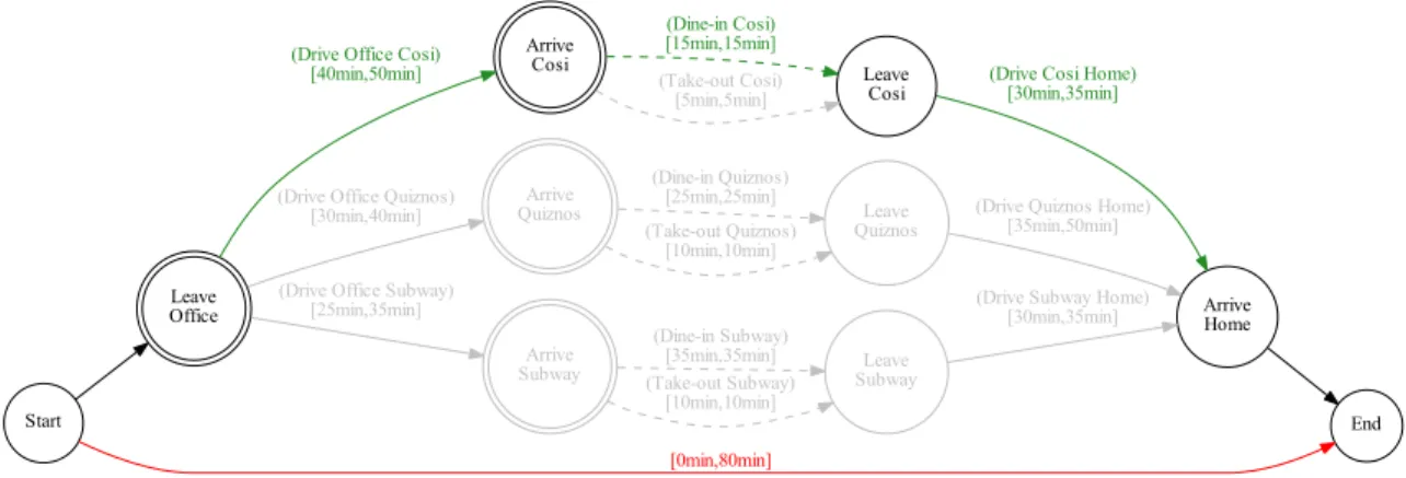
For example, (Figure 2-7) shows a TPN Of candidate plans for to John’s trip problem. It encodes six temporal plans that may satisfy John’s goals. He can have dinner at Quiznos, Subway or Cosi. At each restaurant, he has two options: take-out and dine-in. Instead of creating one choice followed by six independent temporal plans, the TPN uses nested sub plans to make the representation compact. John will only eat at Quiznos if he chooses to drive to Quiznos after he leaves the office (The Choice at event ”leave office”). Otherwise, the sub plan of activities ’Drive to Quiznos’, ’Dine-in’ and ’Drive Home’ will not be activated and executed.

In the TPN, the activities are represented by green arcs with PDDL actions and duration labels. There are four choices in the TPN: ’LeaveOffice’, ’ArriveCost’, ’Ar-riveQuiznos’ and ’ArriveSubway’. They are represented by double circles in the graph.

Start Leave Office End [0min,80min] Arrive Cosi

(Drive Office Cosi) [40min,50min]

Arrive Quiznos

(Drive Office Quiznos) [30min,40min]

Arrive Subway

(Drive Office Subway) [25min,35min] Leave Cosi (Dine-in Cosi) [15min,15min] (Take-out Cosi) [5min,5min] Arrive Home

(Drive Cosi Home) [30min,35min] Leave Quiznos (Dine-in Quiznos) [25min,25min] (Take-out Quiznos) [10min,10min]

(Drive Quiznos Home) [35min,50min] Leave Subway (Dine-in Subway) [35min,35min] (Take-out Subway) [10min,10min]

(Drive Subway Home) [30min,35min]

Figure 2-7: The Temporal Plan Network for John’s trip

John can select one of the three restaurants to go to after leaving the office, and he can choose to dine-in or take-out when he arrives at a restaurant.

In total, the tpn encodes six candidate temporal plans for John to choose from. A temporal plan is like a TPN without any choices, therefore all activities and events are activated. To extract a temporal plan from a TPN, one may make a set of Make a set of assignments to the choices of the TPN to eliminate contingencies.

Definition 9. (An assignment of choices in TPNs) A choice to a TPN is a pair < de, sp > where:

• de is a decision event with domain DSP. • sp is a sub plan and sp ∈ DSP.

However, not all choice sets to a TPN result in a temporal plan. A set of choices is valid only if it is complete.

Definition 10. (Assignments to TPNs) A set of assignments, θ, to a TPN is com-plete if and only if:

• There is no decision event that is activated by θ but not assigned.

• All decision events in θ must be either always active or activated by one of the choice in θ.

A set of assignments to a TPN is incomplete or partial if there is a decision event that is activated [14] but not assigned.

A set of assignments to a TPN is superfluous if there is a decision event that is assigned but neither activated by one of the choice nor always active. An event is always active if it is activated in all sub-plans regardless of the choices made to the decision events.

Note that the completeness of A choice assignment is different from the complete-ness of temporal plan. A complete set of choices to a TPN will result in a temporal plan that supports the goals of the QSP. Such a temporal plan is called a candidate temporal plan of the TPN:

Definition 11. (Candidate Temporal Plans of a TPN) A Candidate Temporal Plan, P, of a TPN, N is a temporal plan where:

• P’s events, E, is a subset of the events in N .

• P’s sub plans, SP, is a subset of the sub plans in N .

• P’s temporal constraints, T C, is the same as the temporal constraints in N . • E, SP and T C can be activated by one complete set of choices to N .

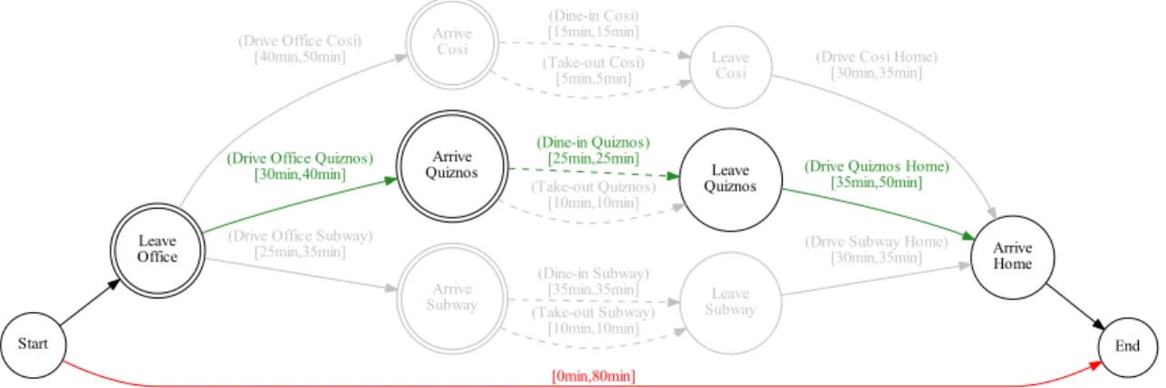
A TPN may have multiple candidate temporal plans, depending on the number of choices and the domain size of each decision events. For example, (Figure 2-8) is a candidate temporal plan of the previously mentioned TPN. It takes John to Quiznos and has join dining in at the restaurant.

Further, the solution to a QSP can be defined as a complete and consistent TPN, in which the state and temporal constraints specified in the QSP are satisfied by at least one of the candidate plans of the TPN. For example, (Figure 2-7) is a consistent TPN, and is complete with regarding to the temporal planning problem with John’s goals specified in (Figure 2-1).

Start Leave Office End [0min,80min] Arrive Cosi (Drive Office Cosi)

[40min,50min]

Arrive Quiznos

(Drive Office Quiznos) [30min,40min]

Arrive Subway (Drive Office Subway)

[25min,35min] Leave Cosi (Dine-in Cosi) [15min,15min] (Take-out Cosi) [5min,5min] Arrive Home

(Drive Cosi Home) [30min,35min] Leave Quiznos (Dine-in Quiznos) [25min,25min] (Take-out Quiznos) [10min,10min]

(Drive Quiznos Home) [35min,50min] Leave Subway (Dine-in Subway) [35min,35min] (Take-out Subway) [10min,10min]

(Drive Subway Home) [30min,35min]

Figure 2-8: One temporal plan for John’s trip

A TPN is complete if at least one of its candidate temporal plans is complete. A TPN is consistent if at least one of its candidate temporal plans is consistent. Finally, similar to over-constrained temporal plans, we can define over-constrained TPNs:

Definition 13. (Over-constrained Temporal Plan Networks) A temporal plan network T PN is over-constrained if none of its candidate temporal plans is both complete and consistent, but at least one of them is an over-constrained temporal plan.

2.3

Failure When Generating Complete and

Con-sistent Plans

Recall that our problem of relaxing a QSP is driven by the fact that the QsP as given can’t be solved. Specifically, there are some temporal planning problems for which no temporal plan can be found to satisfy all state and temporal constraints in the problem. Such a problem is called an infeasible temporal planning problem. In this section, we define the feasibility of temporal planning problems using temporal plans. Further, if a problem is infeasible, it indicates that there are conflicts between the goals specified in its QSP. These conflicts provide useful clues about where to relax the QSP. We discuss two possible causes of failure in this section based on the type of conflicts.

2.3.1

Defining the Feasibility of Qualitative State Plans

Given a temporal planning problem, we define its feasibility based on the solution that can be generated by a planner:

Definition 14 (Feasible QSPs). A QSP, Q, is feasible if and only if there exists a temporal plan, P where:

• P is complete. It satisfies all the state and temporal constraints specified in the QSP of Q: the state trajectories generated by the activities in P satisfy the state constraints, and the state and end time of the state trajectories satisfy the temporal constraints. In other words, P |= Q.

• P is consistent. There is no logical inconsistency between the activities and temporal constraints in P. Every precondition has an action that precedes it, which produces the effect that is desired by the precondition.

Otherwise the QSP is said to be infeasible.

• Given a planning problem, Q, no complete temporal plan can be found that entails all the state and temporal constraints in Q.

• Given a planning problem, Q, there exists a complete temporal plans, P, that can satisfy all the constraints in Q. However, none of the plans in P is consistent. • Given a planning problem, Q, there is only a set of incomplete but consistent plans, P. All plans in P are consistent, but cannot satisfy all the constraints in Q.

We may further divide the second category based on the type of inconsistencies: Q may have complete but temporally inconsistent plans, meaning that some of the temporal constraints are violated; or complete but state inconsistent plans, meaning that some of the preconditions or maintenance conditions of activities are violated.

2.3.2

Outputs of a Planner Given an Infeasible QSP

In this subsection, we discuss the reasonable outputs of temporal planners when giving different QSPs. Throughout this thesis, we assume that there exists an algorithmic planner that can differentiate these types of infeasible problems. More specifically, given a temporal planning problem Q, there are four possible outputs:

• a complete and consistent temporal plan, if the problem is feasible. • a complete but inconsistent temporal plan, if the problem is infeasible. • an incomplete but consistent temporal plan, if the problem is infeasible.

• a signal of failure, if the problem is infeasible and no complete plan and consis-tent plan exists.

A temporal planner will always try to give a complete and consistent temporal plan as the solution to the planning problems. However, no such plan exists if the problem is infeasible. An infeasible temporal planning problem is the result of the conflicts between the goals specified by the user and the planning domains. In other

words, what the user asks for cannot be supported by the planning domain. We list three possible outputs of a planner above if the planning problem is infeasible.

First, if the planner cannot find a consistent plan that can satisfy all the con-straints in the QSP, but only a subset of the concon-straints, it will return an incomplete but consistent temporal plan. It indicates that the options in the planning domain are insufficient for satisfying all the state and temporal constraints of the problem, and it requires the user to supply more options in order to produce a plan.

For example, the robot in (Figure 2-9) is going to move from room A to room B. There is a door in between, but the robot does not know how to open it: the action ’open door’ is not defined in its planning domain. Therefore, a planner would fail to generate a plan that can take the robot from room A and room B. This is the case where no complete plan exists given a planning problem.

A

B

Figure 2-9: Plan failure caused by insufficient options

Second, if only complete but inconsistent temporal plans can be found with respect to the QSP of Q, it indicates the planner can generate a set of activities that satisfies the state and temporal constraints. However:

• A. Some of the preconditions or maintenance conditions of the activities do not hold, or