Continuous curved near wake analysis for a lifting surface

Continuous Curved Near Wake Analysis for a Lifting Surface

by

Melinda Dee Godwin

B.S., Aeronautical Engineering, University of Maryland (1989)

Submitted to the Department of Aeronautics and Astronautics in Partial Fulfillment of the Requirements for the Degree of

MASTER OF SCIENCE IN AERONAUTICS AND ASTRONAUTICS at the

MASSACHUSETTS INSTITUTE OF TECHNOLOGY

September 1991

© Massachusetts Institute of Technology, 1991. All rights reserved.

.1/

Signature of Author

Departme( t-f -ero Iutics and Astronautics July 22, 1991 Certified by

Accepted by

Professor Mark Drela Thesis Supervisor

S

CONTINUOUS CURVED NEAR WAKE ANALYSIS FOR A LIFTING SURFACE BY

MELINDA DEE GODWIN

Submitted to the department of Aeronautics and Astronautics on July 22,1991, in partial fulfillment of the requirements for the Degree of Master of Science in Aeronautical Engineering.

Abstract

Accurate modeling of the near wake remains a significant problem in helicopter rotor aerodynamics. Motivated by the inability of present models to achieve close agreement with experimental near-wake geometries, an improved representation of the near-wake of a one-bladed rotor is developed. Although this problem has been addressed by others, close agreement with experimental wake geometries has not been achieved.

A major problem in matching experimental results using filamentary models involves specification of the proper vortex core size for a curved point vortex. This arbitrary core size is needed to eliminate the logarithmic induced velocity singularity and solutions have been shown to vary significantly depending on the chosen value. The present study uses a continuous vortex sheet rather than discrete filaments, avoiding the need for a finite core size. The model represents a one-bladed hovering rotor trailing a continuous vortex sheet. A free-wake analysis using the Biot-Savart law is then applied to determine the wake geometry in a fixed plane perpendicular to the initial position of the blade. The singularity associated with the circulation distribution at the tip is represented using a self-similar solution developed by Pullin. Several circulation distributions are studied, including an elliptical distribution and a distribution typical of a hovering rotor. For the latter, the intent is to study the character of the vortex roll-up and to determine if, counter to experimental evidence, a mid-span vortex occurs as it has using past models.

Results from the current study may be used in conjunction with discrete models to predict the proper core size to be used. In this manner, the greater computational efficiency of discrete models may be retained while obtaining the accuracy of a more rigorous near-wake

representation. This research could also be extended to forward flight and incorporated in an existing full-wake analysis code as the near-wake component.

Table of Contents

A b stract ... ... ... 3

A cknow led gm ent... ... 6...

L ist of F igures ... ... 7

Nomenclature ... ... 8

1. Introduction ... ... 9

1.1 H istorical N ote ... 9

1.2 Previous Rotor Wake Research ... ... 1.3 Outline of the Present Research ... ... 11

2. Description of the Model ... 1 2 2.1 Coordinate System... 3

2.2 Non-Dimensional Parameters ... 1 5 2.3 Definition of Linear Region ... ... 17

2.4 Exponential Stretching Technique ... 19

2.5 Pullin Similarity Solution ... ... ... 2

2.6 Vortex Sheet Model ... 25

3. A nalytical M ethod... ....2 6 3.1 Application of the Biot-Savart Law ... 26

3.2 Axial Velocity Component... ...3 1 3.3 Radial Velocity Component...3 9 3.4 Tangential Velocity Component...4 3 3.5 Self-Induced Velocity of the Tip Vortex ... 4 3 3.6 Sm oothing ... 4 4 4. An Elliptically Loaded Blade... .. ... 45

4.1 Effect of Smoothing ... 46

4.2 Dependence of Wake Solution on Time Step...4 8 4.3 Dependence of Solution on Linear Region Size...5 0 4.4 Calculated Wake Geometry...5 2 5. Translating Circular Disk ... 56

6. Typical Hovering Rotor Loading... 60

8. Conclusions and Future Recommendations ... 6 R eferences ... 6 6 9 Appendix - Computer Programs ... 7 1

Acknowledgment

My sincerest thanks to my advisor, Mark Drela, for all the time

and effort he spent assisting me in developing this thesis. His wisdom and patience was greatly appreciated.

I would also like to thank the NSF PYI Program, along with Earl Murman and NASA Langley (NASA Grant NAG-1-507) for making this research and my masters possible.

Finally, I would like to thank my husband Mark for his support, assistance, and understanding through the final stages of this thesis.

List of Figures

Figure 2.1-1 Basic Coordinate System ... 1 4 Figure 2.1-2 Definition of s Coordinate ... ... 1 4

Figure 2.1-3 Top View of Rotor... 5

Figure 2.3-1 Determination of Linear Region Size ... 8

Figure 2.4-1 Filament Distribution ... 20

Figure 2.5-1 Pullin Solution Applied to Elliptically Loaded Blade...24

Figure 3.1-1 Problem Set-Up ... ... 28

Figure 3.1-2 Application of Biot-Savart Law ... 30

Figure 4.1-1 Effect of Smoothing ... ... 47

Figure 4.2-1 Effect of Time Step... 49

Figure 4.3-1 Effect of Linear Region Size ... .. 5 1 Figure 4.4-1 Wake Profiles for the Elliptically Loaded Blade...5 3 Figure 4.4-2 Wake Profiles for the Elliptically Loaded Blade ... 5 54 Figure 4.4-3 Wake Profile for the Elliptically Loaded Blade, 'F = 450...5 5 Figure 5-2 Circulation & Wake Distribution for the Oblate Spheroid...5 8 Figure 5-3 Downwash Distribution for the Oblate Spheroid...5 9 Figure 6-1 Typical Hovering Rotor Circulation & Wake Distribution...6 1 Figure 6-2 Wake Profile for Typical Hover Circulation, 'P = 100...6 2 Figure 6-3 Wake Profile for Typical Hover Circulation, P = 200...63

Figure 6-4 Wake Profile for Typical Hover Circulation, P = 300...6 4

Nomenclature

d h segment of integration strip which produces a velocity at a point in space.

I radius vector from dh to a point in space r radial displacement corresponding to s

R radial displacement of marker corresponding to s s location where circular integration strips are located

S location along vortex sheet where induced velocity is calculated z vertical displacement of wake corresponding to s

Z vertical displacement of marker corresponding to s

28 width of linear region

'P rotor azimuthal angle, radians Fb bound circulation

1. Introduction

1.1 Historical Note

Modeling the aerodynamics of a rotor has always been a difficult task due to the geometric and aerodynamic complexity of the wake. In the early 1900's, Kutta and Joukowsky related lift to vorticity in the flow, providing the fundamental basis for vortex modeling of rotor wakes. This approach utilizes the Biot-Savart law which allows determination of the induced velocity at any position in the wake and modeling of the wake deformation and displacement in unsteady flows.

1.2 Previous Rotor Wake Research

Many different analyses and models evolved using vortex modeling, including the vortex sheet and filamentary models discussed below. The most recent development in vortex modeling has been free-wake analysis, defining the complete free-wake geometry using the calculated induced velocities. Free-wake analyses are physically more correct than previous models and, for that reason, many recent studies have been focusing on utilizing and optimizing this method of analysis.

Motivated by the inability of existing models to accurately predict near-wake geometry, this thesis focuses on an improved representation of the near-wake of a one-bladed rotor (the near wake is defined to

extend from I = 00 to T = 450). Although there are a variety of near

wake analysis programs using filamentary and vortex sheet models, the need to specify an arbitrary core size limits their general applicability.

as a series of semi-infinite vortex elements which are then rolled up into two or three discrete vortices (before the first blade is encountered) according to Betz criteria.2_,3 _{Since the mid-span and root} vortices which result have not been detected in any of the relevant experimental studies, Miller states that an "exact prediction of the wake structure" can not be determined from the results, and the roll-up technique should only be viewed as a "convenient computational technique to account for the effects of the inboard trailing vorticity".4

A vortex filament model developed by Brower5 _{considers the} entire rotor wake. Brower represents the near wake as straight vortex segments and includes a correction for viscous core size (causing the induced velocity to approach zero rather than infinity as the vortex element is approached). Since Brower uses straight filaments, he adds a correction factor for self-induced effects, since actual vortex filaments leaving the blade are curved and will induce a velocity on themselves. Brower found that the choice of core size had a significant effect on the induced velocities at nearby points, and that the choice of core size should be related to the computational mesh size. Most papers written on filamentary models note difficulties in selecting a proper core size due to the lack of a physically correct predictive model and an incomplete understanding of how core size is related to specific flows.

Vortex sheet models for near wake analysis using a free-wake approach have also been developed. An example is the model developed by Tanuwidjaja.6 The near-wake is modeled as a vortex sheet with tip and root vortices. This method uses the Biot-Savart law and divides the blade and wake into nodes which define discrete

induced velocities, however, are not calculated at these nodes, due to singularity problems at the discrete sheet elements. Instead, new locations between the nodes called "centers" are defined. The induced velocity is then calculated at these centers and linear interpolation is used to find the velocities at the nodes. Since, however, Tanuwidjaja uses discrete vortex sheet elements, the arbitrariness that stems from the need to specify a finite core size is not eliminated.

1.3 Outline of the Present Research

In this study, unlike the iterative analyses by Miller, the model is given a circulation distribution that is assumed- correct, and it then calculates the induced velocities and resulting wake geometry by integrating across the wake using the Biot-Savart law. The induced velocities in the wake are calculated at sequential increments in time, so "snap-shots" of the resulting wake geometry are obtained downstream of the rotor. This process is repeated until an azimuthal angle of 1F=45 degrees is reached. This is a continuous model, therefore no finite core size (except for the tip vortex) is needed, which eliminates the arbitrariness in the solution due to core size specification.

As previously stated, the present research considers the near wake of a one bladed rotor using a free-wake analysis. The entire wake geometry is not considered, since the intermediate and far wakes are comparatively well understood (although computationally time consuming to analyze)7_{. Rather it is the intent to focus on a more} physically correct representation of the near wake, yielding results which more closely match experimental data. By obtaining a more

accurate near wake geometry, this program may be utilized in the following ways.

1. To assist in selecting the appropriate core size to be used in

filamentary models where core size is included as a parameter. 2. To test other wake geometry programs to investigate the accuracy

of their solutions.

3. As the near-wake component in a full-wake analysis code.

Miller states, "It will never be possible to model exactly the dynamics and aerodynamics of a system as complex as a rotary wing vehicle. .... To this end the simplest forms of analysis, which retain the essence of the phenomena involved, are of greatest value during the crucial stages of design and flight evaluation."8 _{The difficulty lies in} knowing how to simplify a model while maintaining an acceptable level of accuracy. While the model outlined in this thesis may be physically more correct, it may not be practical to efficiently implement in free-wake codes modeling the entire free-wake. The model is more computationally time-consuming and mathematically difficult than models such as Miller's fast free wake analysis. The best alternative would be to use the knowledge gained from this research to improve the results of more simplistic models, thereby achieving good results while minimizing computational expense.

2. Description of the Model

The present axisymmetric model represents the near wake of a one bladed rotor as a vortex sheet rather than by a series of discrete

filaments. This sheet is composed of 500 integration intervals which contain the vorticity in the wake. In reality these integration strips follow helical paths downstream of the rotor. Miller has shown, however, that the effect of the inclination of these integration intervals on the induced velocity is negligible.9 _{This model is therefore} developed using integration intervals which are planar circles perpendicular to, and centered about the z-axis (see figure 3.1-1). This results in an axisymmetric flow pattern where the axial, radial, and tangential velocity components are independent of I'. Since the circular integration intervals remain perpendicular to the axis of symmetry as the wake convects downstream, the tangential component of the velocity will always be negligible. The purpose of this model is to investigate how the wake deforms downstream of the rotor blade, and to develop insight into the question of whether or not a discrete mid-span vortex is formed. First, a description of the coordinate system is provided, followed by an explanation of the primary non-dimensional parameters. The "linear region" concept used to eliminate the computational singularity in the induced velocity equations is then described. _{Next, the exponential stretching technique used to define} integration strips (containing the vorticity in the wake) is discussed along with the similarity solution developed by Pullin to handle the tip singularity. Finally, a description of the vortex sheet will be given.

2.1 Coordinate System

The coordinate system for the wake geometry used in this analysis is three-dimensional, consisting of radial (r), azimuthal (I) and vertical (z) components, as shown in figure 2.1-1.

SIDE I ' = 0-45 o .. ~ No,•-Z Figure 2.1-1

- r

Basic Coordinate System

The actual wake deformation is viewed in two dimensions in the r-z plane (as shown in the side view above), producing two-dimensional, time dependent wake profiles. To designate locations along the profile, a sheet coordinate, "s", is introduced.

SIDE VIEW

Blade

s

Figure 2.1-2 Definition of s Coordinate

To simplify the form of the equations, it is assumed that the

two-I- m -

-C TOP

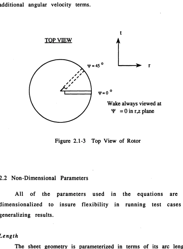
-the blade moving away at a positive angle. additional angular velocity terms.

This approach eliminates

TOP VIEW

= 45 o

'I=0o

Wake always viewed at T = 0 in r,z plane

Figure 2.1-3 Top View of Rotor

2.2 Non-Dimensional Parameters

All of the parameters used in the equations are non-dimensionalized to insure flexibility in running test cases and generalizing results.

Length

The sheet geometry is parameterized in terms of its arc length s, non-dimensionalized by the blade radius. The sheet geometry is

therefore defined by the coordinates r(s) and z(s), which are also non-dimensionalized by the blade radius.

In the numerical scheme, the marker locations on the sheet where the velocity is calculated are denoted by uppercase symbols S, R, and Z, while the locations of the integration strips containing the vorticity are denoted by lowercase s, r, and z.

marker r-location marker z-location

blade radius = blade radius

Angle

The angle P refers to the azimuthal angle (in radians) about the axis of rotation extending from -x to x. This angle is shown in Figure 2.1-3.

Time

Time is non-dimensionalized by 0, the rotational speed of the

rotor (i.e. t* = t Qi). As an example, an azimuthal angle of xt/4 radians

corresponds to a non-dimensional time t*=,x/4, or more generally, At*=A'Y. The near wake is broken into 45 increments, and therefore the outer time loop in the program moves through 45 one-degree time steps.

Velocity

The dimensional velocity is simply the ratio of the non-dimensional length and time described above:

V* = _{l*/t* - (blade radius)(t)(G) (Q)(blade radius)}

2.3 Definition of Linear Region

The linear region is a specified area on either side of a marker within which the equations are modified to analytically remove the singularity that occurs when an integration interval approaches a marker location.

It is necessary to integrate equations 3.14 and 3.30 over the sheet length s, since the r and z terms are both functions of s. To facilitate this integration, r and z terms are linearized with respect to s. This is accomplished through the following relations:

R-r = KI(S-s) Z-z = K2(S-s)

dr dr

where K1 = dss=S K₂ =ds 's=S

These linear relations are then used to eliminate r and z in the equation, resulting in an equation dependent only on s. This allows the singularities in the integral to be analytically removed. Since these equations (i.e. 3.14, 3.30) can only be defined over small portions of the wake (because of the linearizations above), the modified form of the equation is only used when an integration interval is in close proximity to a marker (in the linear region) and the unmodified original equations are used elsewhere. The size of the linear region is a variable, and it

will be shown that the wake geometry is independent of the precise value chosen as long as the linearity assumption for r and s, and z and s remains valid. For the test cases shown, the lesser of the two distances

from the marker being considered to the markers on either side is chosen as 8 and the linear region is twice this distance (half on each side of the marker as shown in figure 2.3-1).

Marker Under Consideration SO-1) S(j) S(j+1) .02 .03 Linear Region 8 = MIN(0.02, 0.03) = 0.02 Slow = S(j) - 8 Shigh= S(j) + 8

width of linear region = 28

Figure 2.3-1 Determination of Linear Region Size

In summary, the linear region represents a specified area about each marker within which the governing equations are modified to eliminate the singularity which would otherwise occur as an integration interval approaches a marker. The only difference between the

modified and unmodified equations is the elimination of higher order terms.

2.4 Exponential Stretching Technique

Layout of Markers

An exponential stretching technique is used to construct the initial lay-out of the markers (i.e. the locations where induced velocities are calculated). The stretching technique requires as input the desired number of markers and the desired distance between the first two and the last two markers. The routine then exponentially stretches between the second and the second to last markers. In general, a large distance between the first two points is specified and a small distance between the last two points. This results in a low population of markers near the root and a high density layout at the tip where, due to the tip vortex, the curvature of the wake is greatest (150 markers are generally used).

The vortex core, which is used as a filament and a marker, is not located through this technique, but through a method outlined in

section 2.5.

Layout of Integration Strips Containing the Wake Circulation

The layout of the integration strips, unlike the layout for the markers, is modified at each time step and for each marker. At each time step, the sheet is broken* into integration intervals to account for the vorticity in the wake. These intervals need to be denser near the tip (due to the strong vorticity and roll-up) and near the marker under consideration (due to the possibility of a singularity point being

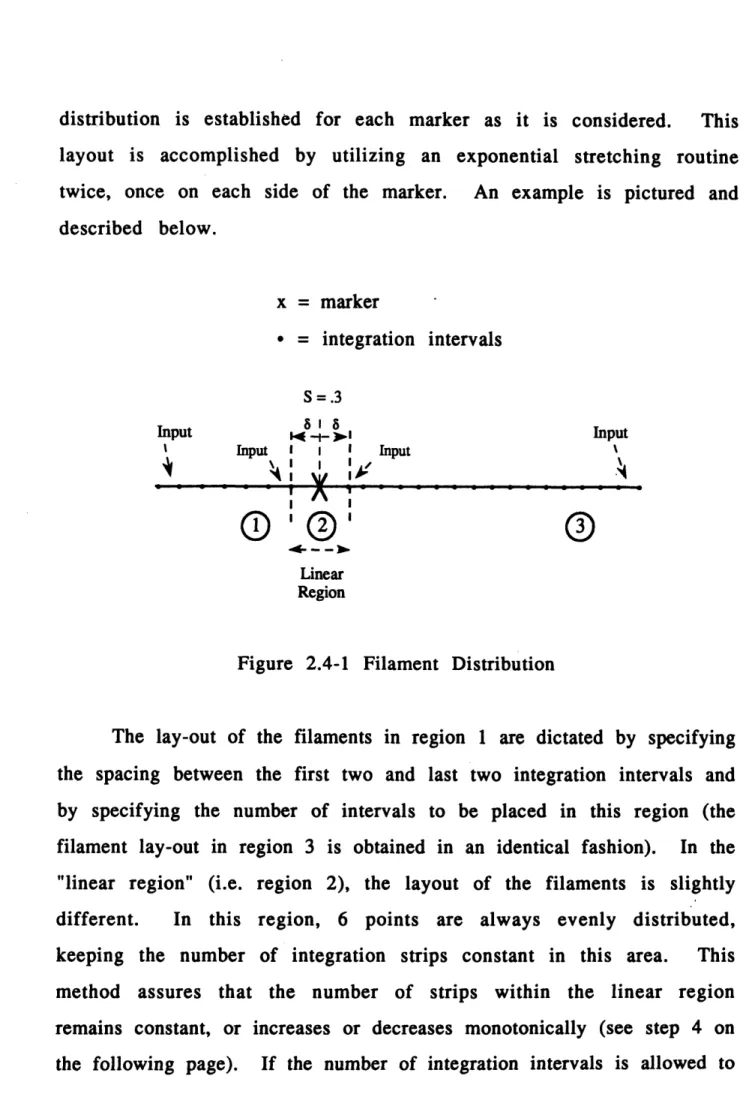
distribution is established for each marker as it is considered. This layout is accomplished by utilizing an exponential stretching routine twice, once on each side of the marker. An example is pictured and described below. x = marker = integration intervals S = .3 Input -- • Input Input I I I Input I I Linear Region

Figure 2.4-1 Filament Distribution

The lay-out of the filaments in region 1 are dictated by specifying the spacing between the first two and last two integration intervals and

by specifying the number of intervals to be placed in this region (the

filament lay-out in region 3 is obtained in an identical fashion). In the "linear region" (i.e. region 2), the layout of the filaments is slightly different. In this region, 6 points are always evenly distributed, keeping the number of integration strips constant in this area. This method assures that the number of strips within the linear region remains constant, or increases or decreases monotonically (see step 4 on

randomly fluctuate, instabilities occur in the wake due to truncation errors. These truncation errors arise due to the loss of higher-order terms, which occurs because the equations used in the linear region have been modified to handle the singularities which arise in this area. The lay-out of the filaments can be summarized as follows:

1. The linear region variable (8) is added and subtracted from each side

of the marker.

2. The area from the root to the left end of the linear region is stretched, and integration strips are located.

3. The area from the right end of the linear region to the tip is stretched

and integration strips are located.

4. Six integration strips are located in the linear region, equal distances apart. At the root and the tip, where the linear region is only one-sided, 4 integration strips are used.

5. The midpoints between all these locations are then taken, starting

from the root of the blade. These midpoints define the locations of the integration intervals.

6. This 5 step process is then repeated for each marker, at every time

2.5 Pullin Similarity Solution

Due to the singular roll-up at the outer edge of the sheet, a discrete tip vortex forms instantaneously. Applying the Biot-Savart law directly without accounting for this singularity leads to erroneous results. One way to resolve this singularity is to use the self-similar solution developed by Pullin.10,11 Pullin considers a semi-infinite vortex sheet with F=2alRI1/2 (where R is the location along the blade, and "a" is a scaling parameter), and develops a self-similar solution which produces an initial wake geometry and circulation distribution past a certain matching point (in this case r/R=0.95) at time r=0+. Pullin derives a similarity solution where:

Zo(F,,) = (at)2/3 C(() (1) and

r

Zo: dimensional self-similar shape function for

the sheet.

Using Pullin's solution along with initial values for ý and X (obtained by choosing a matching point along the vortex sheet), the above two equations can be solved for t and a (the scaling parameters), yielding the initial circulation distribution and wake geometry beyond r=0.95 for

S= 0+. An example is given below for the circulation distribution F(r) =

.02ý1-r, where ýo = -3.24R and 1o=3.6, and s=0.95 where s is the location along the sheet defined as the matching point.

(1) Substitute F and Z into (1) and (2):

Zo3/2 [(1-S)]3/2

t 3/2 a (3.24) 3/2 a (la)

Note: (1-s) is necessary because Pullin has 4=0 at the tip, and the coordinate system in this thesis is opposite.

3

t =

(X3 a4)

(.02 1-(1-s)2) 3

(3.6)3 a4

(2) Solve(la) and (ib) for t and a. In this case t = 0.1373 and a = 0.01396.

(3) Using t and a, the wake geometry and circulation distribution are

defined beyond 95% blade radius by scaling Pullin's solution accordingly (see figure 2.5-1).

CIRCULATION INPUT FOR ELLIPSE

0.34 0.67 1.01

INIT WAKE INPUT FOR ELLIPSE

0.933 0.967 1.0( 0.0200 0.0133 GAMMA 0.0067 0.0000 INIT WAKE o o VORTEX POS 18 Jul91 13:24:20 18 Jul 91 13:24:20 18 Jul 91 13:23:21

Figure 2.5-1 Pullin's Solution Applied to an Elliptically Loaded Blade

CIRCULAT 0 00 -0.050 -0.017 Z 0.017 0.050

INITIAL WAKE FOR ELLIPTICAL DISTRIBUTIC AFTER SCALED BY PULLIN'S SOLUTION

0.900

(4) Determine the tip strength and location. Pullin gives the total value of X for the four spirals and the core as 1.342. By dumping this

circulation into the core and re-locating the core (although in this case the amount the core is moved is negligible), the core strength is found to be X=1.342 and its location is C = -.308_{er, ii = .498ez, whose} values can be scaled to F, z and r values.

One problem encountered when using this solution is in step 3 where Pullin's solution is scaled for the appropriate test case. Since Pullin's wake and circulation distribution were not available in tabular form, several values were estimated from the plots in references 10 and

11 and then splined. Due to unavoidable errors in transcribing this data, however, small perturbations would amplify and the wake would rapidly go unstable. To resolve this problem, Pullin's solution is applied to a specific case study (in this instance the ellipse), and then the resulting wake and circulation distributions are fitted with equations.

By using the data from these equations (which contains the Pullin

solution), the singularity due to dF/dr approaching infinity at the blade tip is eliminated and an initial wake geometry and circulation distribution are defined.

2.6 Vortex Sheet Model

The basic wake model consists of a continuous vortex sheet with a discrete tip vortex. The wake is defined by two independent parameters, R and Z, where markers are placed. These markers are also

therefore the points tracked downstream of the rotor blade which define the wake evolution in time. The number of markers used to represent the wake is a variable. Two other important parameters used throughout the analysis, r and z, are variables of integration, and represent the location of the integration strips containing the vorticity in the wake. The remaining two sheet geometry parameters are S and s, both referring to the sheet coordinate. The parameter S is the actual location of the markers along the sheet, while s is the location of the integration strips along the sheet. The number of integration strips is also a variable. These integration strips are modeled as circles from

P=-x to Y=ni as shown in figure 3.1-1. Relating these six parameters:

AS2 = AR2 + AZ2 As2 = Ar2 + Az2

3. Analytical Method

3.1 Application of the Biot-Savart Law

The two-dimensional near-wake geometry is obtained using a free-wake analysis technique. Using this approach, the wake assumes an equilibrium (or "force-free") position by moving according to the induced velocities at each marker location. These velocities are obtained by applying the Biot-Savart law at each marker and integrating along the sheet.

The wake is composed of circular integration intervals containing the circulation in the wake. These intervals are of infinitesimal strength

intervals rather than vortex filaments, since they do not require a finite

core size, as is the case with conventional filamentary models. In this continuous sheet model, the coordinate s is defined positive outward along the sheet. The location of the circular integration strips along the sheet are defined by lower case s, while the locations of the markers, where the induced velocities are calculated, are defined by S (see figure

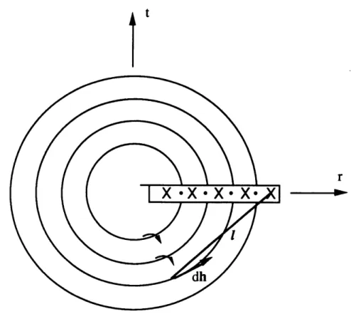
TOP VIEW .ATION STRIP

I

To calculate the induced velocity at any point in the wake due to a filament of strength F, the Biot-Savart law can be applied as follows: 12

F

rdh

x

I

dxV

4n

1113

F: strength of the vortex filament.

dh: segment of the filament which induces a velocity at a point in space.

1: radius vector from dh to any point in space.

Application of the Biot-Savart Law

For a vortex sheet composed of circular integration intervals initially in the plane of the rotor, this equation becomes (see figure

3.1-2):

Vi dF 1 dh

ds

t

r

A

Figure 3.1-2 Application of Biot-Savart law

Now referring to figures 3.1-1 and 3.1-2 and realizing there is an additional component of the 1 _{vector in the z-plane at all times after r=0,}

it is clear that:

1 = {R-r cos})r - (r sinP}t + {Z-z}z _(3.3)

Since the dh vector in equation 3.2 is tangent to the circular integration strips (which remain parallel to the rotor plane at all times downstream), it is only composed of components in the r-t plane. This vector can be represented as:

Therefore, after computing the cross-product dh x 1 and substituting back into the Biot-Savart law (equation 3.2) the following equations are obtained:

1S

V

=

axial induced velocity = 4I dss

Vr = radial induced velocity = - 4 ds

0

1 s Vt = tangential induced velocity = -- 4

0

SR

cos'-r

-X

These equations represent the radial, axial, and tangential induced velocities calculated at each marker location.

3.2 Axial Velocity Component

As shown above, the equation derived for the axial velocity using the Biot-Savart law is:

d=JrJ

4xVa f

ds

rf

d sr

R cos(P) - r

13= R2 _{- 2Rr cosY + r}2 _{+ (Z-z)}2 _}3/2

Now defining F as:

R cos(Y) - r

F= I3_Ill3

and substituting Il13 into this expression, F becomes:

R cosy - r F= [R 2_{- 2Rr cosY}

+ r2 + (Z-z)2]3/2

It is apparent that a numerical singularity is encountered when cosy approaches 1, and r approaches R (when r=R, z=Z). To resolve this

T2

singularity, cosW=1 - 2 may be substituted into 3.11 to yield the factor which must be added and subtracted to F so the equation is well-behaved. Upon completing this substitution, it is apparent that the factor H (defined below) when used as shown in 3.13, eliminates the singularity in 3.11. R-r H = [(R-r)2+Rr?2+(Z-z)2]3/2 (3.12) 4Va=j r [F(r,R,)H(r,R,)-H(r,R,)] Jdds + j - rfH(r,R,T)dYds (3.13) (1) (2) (3) where: (3.9) (3.10) (3.11)

In this manner, as cosI approaches 1, and r approaches R, the numerator and denominator of the first two terms in 3.13 approach zero at the same rate. The third term in equation 3.13 is now integrated analytically with respect to TY from -x to x and defined as "A" where: ds r(R-r)2x ds A =JH(rR,)d d=(R-r)2 [(R-r)2 + (Z-z)2] [(R-r)2 + (Z-z)2 + RrX2]1/2 (3.14)

This analytical solution (3.14) now must be integrated over s numerically. Once again, however, the denominator goes to zero faster than the numerator as r approaches R (as an integration strip approaches a marker). The elimination of this singularity is slightly more complex because the integral is over s, and the relationships between r and s, and z and s are known only in spline form. To solve this problem, the r and z terms are linearized with respect to s as outlined in section 2.3. In this manner, r and z can be represented as simple linear functions of s, and the integration of equation 3.14 with respect to s becomes straightforward. This linearization and the modified form of 3.14 that follows will only be used over the linear region. At all other locations along the vortex sheet, equation 3.14 will be integrated numerically in its original form.

The linear relations defined in equation 2.3.1 will now be substituted into 3.14 for integration over s, resulting in:

dF

Alin = 2xI ds KI[R-KI(S-s)] ds

C(S-s)[C(S-s)2 + R 2 t 2 - R K 1(S-s) t 2]1/2 where: dr

K

ds s=S

Before the integration over s can be completed, however, it is apparent that an additional term B (below) needs to be added and subtracted from Alin to avoid the singularity which occurs as s approaches S:

(3.16)

2K

_Id

_s

B=-C(S-s)

Equation 3.15 can now be integrated over s from 0 to smax, and the third term in equation (3.13) results in:

dr

r''AsI _{d-- r(R-r)21L}

r Ads = z)2_{] [(Rr)}2_{+(Z/2 ds}

ds

[(R-r)2+(Z-z)2] [(R-r)2+(Z-z)2+Rr(x)2]1/2

3.15 + 3.16 - 3.16 =

(3.17)

dr

dr

dr

within the linear region.

In the last term of 3.18, s8 1 refers to the first integration strip encountered inside the linear region, and s82 refers to the last integration strip encountered inside the linear region.

When considering a specific marker and stepping through the integration strips (i.e. integrating along the sheet), 3.17 is used until s comes within + or - 8 (which defines the linear region- see figure 2.4-1) of the marker. At this point, 3.18 is used until this linear region is exited, and then use of 3.17 is resumed.

Now reviewing the first two terms in 3.13 (F-H) there is one more singularity to be eliminated. This is again resolved by substituting cosT' = 1- (1/2)T 2 _{in the numerator and denominator of F (as shown in 3.19)}

to yield the additional term needed to eliminate the singular behavior of equation 3.19. Ry2 R- - r 2 R - r F-H 2-_ [R2_+r2_-2Rr+RrP 2_+(Z-z)2_{]3/2 - [R}2_+r2_-2Rr+RrP 2_+(Z-z)2_]3/2 (3.19)

The two terms in 3.19 will not cancel unless R'Y2_{/2 is included in the} numerator of the second term. This factor must also be subtracted from

3.19 so the equation remains unchanged. Therefore: F-H = R cos(Y) - r [R2- 2Rr cosY + r2 _{+ (Z-z)} 2_]3_/2 _" RyF2 R-r-2 [R2 + r2 - 2Rr + RrP 2 + (Z-z)2]3/2 -R'y2 2 [R2 + r2 _{- 2Rr+ RrP} 2 _{+ (Z-z)}2_]3_/2 _(3.20)

The first two terms of equation 3.20 will now be renamed F-H'. The third term of equation 3.20 is integrated analytically over T and becomes:

r[(R-r)2 + (Z-z)2 + Rr(x)2]1/2

log + X2 (R-r)2+(Z-z)2

2r Rr g Rr

log -X + X+ Rr

J

All terms in 3.21 will be well-behaved when integrated along the

Taylor's Series expansion, which reveals the additional term to be added and subtracted from this function so it becomes well-behaved.

resulting third term in 3.21 is:

X2

+

[(S

- s)2

R[R-kl(S-s)]

S+ log I-sR2

2xR2

Because of finite precision arithmetic, (3.22) exhibits noisy when:

K1(S-s)

< 0.01

It is therefore necessary to do an expansion about 1 to the first

K 1(S-s)

log term in 3.22, which will only be used when R < 0.01. This first term becomes:

1

2r_ Rr (3.23)

Defining the total component of axial velocity (including the additional terms so the equation remains well-behaved over the linear region): Va - r (F-H')dT + 4n ds _{r a+b(x)2} The 1 2rIb { (3.22) behavior

-~---Elog(

+ X2

A*]

I

7b

-A*

+

A*

= log

Outside the linear region, however, this equation simplifies to:

a1 Va = I4

41c

2x f

Elog

I

2

7b

log(

_7+b2

)

ds

+

_x

_g

3.3 Radial Velocity Component

The radial velocity component of the induced velocity is derived in a similar manner. First, from the Biot-Savart law, the general form of the radial velocity is:

Vr=I df r cosr(Z-z) dO ds

Vr = - d~s 1113 d ds _(3.26)

where J is defined as:

cos' (Z-z)

[R2_{- 2Rr cosW + r}2 _{+ (Z-z)2]3/2} (3.27)

The singularities in J are analytically removed using equations

3.28 and 3.29. Z-z [(R-r)2+Rr y 2+(Z-z)2]3/2 (3.28) 4xVr = I dff[J(r,R, P) - K(r,R,,P)]d' + IK(r,R, I) dIP} d s (1) (2) ₍₃₎ (3.29)

The third term in equation 3.29 is now integrated analytically over ' and is found to be:

dF

ds 2tr(Z-z)

Al =(3.30)_[(R-r)2 _{+ (Z-z)}2_][(R-r)2 _{+ (Z-z)}2 _{+ Rr(2]1/2}

This equation must now be integrated over s, but singularities are encountered identical to those in equation 3.14 in the previous section. This singular behavior is handled in a similar manner, transforming equation 3.30 into: Ss K2 R-KI(S-s)} ds 2K 2t

fC(S-s)[C(S-s)2

_SlogS-l

S-sl

_I

(3.31)

within the linear region and

dr

J _{ds r}2 _t(Z-z)

2x f

dsz

(3.32)

[(R-r)2 + (Z-z)2] ([(R-r)2 _{+ (Z-z)}2 _{+ Rr(nt)} 2_])1/2 _(3.32)

outside the linear region.

Returning to the first two terms in equation 3.29, J and K, there is one additional singularity which is removed by adding and subtracting 3.33 to J-K which results in equation 3.34.

y%2

(Z-z) 2

(Z-z) 2

The first two terms of 3.34 will now be renamed J-K'. The third term, denoted Dl, is then integrated analytically to yield:

del x

DI=

b [(R-r)2+del2+b()2] 1 / 2

2b-lb [logi + 2+ log -R+ J 2 (3.35)

The third term in 3.35 _{exhibits singular behavior identical to the}

third term in equation 3.21, and is handled in a similar manner (which translates into the B* terms in 3.36). _{The only difference is in the} numerically integrated term which is approximated as zero due to its symmetry about a marker location.

the total component of radial additional terms to eliminate the singularity):

Vr =

_r4

_ds

r (J-K')d

+

R a+Rr(n)2

(Z-z)log(t +

92

)

-lo +

the _program not in the linear region, this equation

dr ((Z-z) ax

r dJ (J-Kbar)dP + z x

L

1

Vr

velocity (including the Defining

dr

a

l(ds

a

r -z

2b4 b b) ds + 2na[a+bx2]1/2 ds

where a= (R-r)2 _{+ (Z-z)}2 _{b= Rr (3.37)}

3.4 Tangential Velocity Component

The general form of the tangential induced velocity, developed using the Biot-Savart Law, is defined as:

Vt

f

r

rsinP(Z-z)

V= -

J

J

This term has negligible effect on the wake geometry for the following reasons. The denominator must be small (or the numerator very large) to obtain a significant component of Vt. Since I (the denominator) is the distance between the interval of integration and the marker position, I is only small when T is near -x or x (see figure 3.1-2). When T is near

-x or -x, however, sinY is appro-ximately zero, so the tangential induced

velocity is always small and has no significant effect on the wake geometry and is therefore ignored. This is one of the bases of the axisymmetry assumption made in this thesis.

3.5 Self-Induced Velocity of the Tip Vortex

Since the tip vortex has a finite strength and is curved, a self-induced velocity term is included. This self-induced velocity is found to be:

w

=

In _}

_(3.39)

where R is equal to the radial location of the vortex and "a" is its core radius. 13

3.6 Smoothing

Under certain conditions, minor instabilities occur in the wake beyond 90% radius. If these instabilities are not eliminated, they are carried into the vortex (as the sheet is stretched) and the vortex roll-up becomes unstable. For this reason, a smoothing routine was introduced. This routine, called filter, uses a second order difference scheme to

smooth certain points in the wake. Filter solves:

d2_r

-t2fil ds2 + r = r

which smooths ro(s) into r(s). This is done in an identical manner for z(s). It is therefore evident that if tfil = 0, then r=r0 and there is no

d2,

smoothing, alternatively if tfil approaches infinity, then ds2 _{=0 (i.e. r(s)} is linear in s, and the wake sheet is "smoothed" straight).

The degree of smoothing is therefore controlled locally by tfil. Tfil is set to a specific value (usually between 0.01 and 0.02) if the marker being considered is in need of smoothing and 0 if no smoothing is necessary.

Although a general criterion was followed in defining tfil as either zero or some finite value, modifications were necessary for each test case as defined below.

Circular Disk Distribution

For this fundamental test case, which looks at the downwash on a translating disk, no smoothing was necessary.

Elliptical Circulation Distribution

Since the elliptical distribution is monotonically decreasing, geometric inflection points in the wake are used to enact the smoothing routine. The markers in need of smoothing are located by considering subsequent sets of four points (forming 3 vectors), and multiplying the cross product of the first and second vectors times the cross product of the second and third vectors. If this product is found to be negative, an inflection point has been located and tfil is set to 0.01 for the marker being considered, otherwise tfil is set to 0.

Miller Distribution

For this distribution there is a natural inflection point in the wake at approximately 95% radius.14 _{To avoid erroneous smoothing in this} area, the smoothing routine used for the elliptical distribution was only applied from 0.96-1.0 R. In addition, a stronger smoothing parameter

(0.015) was used.

4. An Elliptically Loaded Blade

For an elliptically loaded blade at c=0:

r(r) = .02 1-(r)2 r->[0,1]; z=0

Due to the singularity at the tip in the initial circulation distribution, a tip vortex is instantaneously formed. Pullin's self-similar solution is applied here, as discussed in Section 2.5. By following the steps outlined in that section, the scaling parameters a and t are found to be 0.01396 and 0.1373. These parameters are then used to scale the outer portion of the circulation distribution and wake geometry appropriately, while also giving the strength, location and radius of the tip vortex. The resulting circulation distribution and initial wake geometry are shown in Figure 2.5-1.

For this classical case, several issues are investigated as the blade passes through 45 degrees and the wake convects downstream.

(1) effect of smoothing on wake geometry (2) effect of time-step on wake geometry

(3) effect of linear region size on wake geometry

(4) evolution of the wake from P = 0 to P = 45 degrees

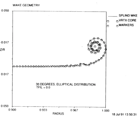
4.1 Effect of Smoothing

As previously stated, the smoothing parameter (tfil) used for this distribution was 0.01. In Figure 4.1-1, the wake at T=30 degrees is shown before and after smoothing.

WAKE GEOMETRY

30 DEGREES. ELLIPTICAL DISTRIBUTION TFIL = 0. 0 , r - " 0. v 00 0933 0 967 1.000 RADIUS I -- -WAKE GEOMETRY __ SPLIND WKE I M VRTX CORE 0 OMARKERS 18 Jul 91 14:30:11 1 000

Figure 4.1-1 Effect of Smoothing Wake Geometry

-0.017 Z/R 0.017 0 050 09 -0 050 -0.017 Z/R 0.017 0.050

30 DEGREES, ELLIPTICAL DISTRIBUTION TFIL = .01 0.900 0.933 RADIUS 0.967 I I11 n n0 m In SPLIND WKE Cq VRTX CORE ( MARKERS 18 Jul 91 13:50:31 ( "V]-I

It is important to note that while all inflections are eliminated, the curvature of the wake and the extent of vortex roll-up are not changed significantly. Originally, a smoothing routine was adapted which smoothed every marker along the sheet, rather than only those near an inflection point. The result was a significant loss of curvature in the wake beyond 95% radius along with a large decrease in the diameter of the vortex.

4.2 Dependence of Wake Solution on Time Step

A Predictor-Corrector difference method was utilized for the

time-step scheme, providing second-order accuracy. The wake was normally set to convect in one degree increments downstream of the blade. To validate convergence, however, half degree time steps were also tested on the elliptical distribution. The resulting wake geometries at various time steps downstream were compared with wake geometries using one degree increments. Figure 4.2-1 shows one of these wake comparisons at 'P=5 degrees. The slight difference seen between the two roll-up's indicates the coarseness of the time step is borderline.

WAKE GEOMETRY SPLIND WKE Fj M]VRTX CORE ( C₀MARKERS 18 Jul 91 13:53:45 1.000 WAKE GEOMETRY -0 050 -0.017 Z/R 0.017 0.050 0.933 0967 RADIUS 1 000 SPLIND WKE SVRTX CORE oMARKERS 18 Jul 91 14:28:24

Figure 4.2-1 Effect of Time Step on Wake Geometry

-0017 Z/R 0.017 0.050 Dj-e 0.900 0 933 RADIUS 0 967 mmmmm

"wf rpn~YY~ImFel"T",npnr

5 DEGREES, ELLIPTICAL DISTRIBUTION HALF DEGREE TIME STEP

4.3 Dependence of Solution on Linear Region Size

The linear region, as explained in Section 2.3, is a region where the equations for the induced velocity are modified to eliminate singularities that arise as a variable of integration approaches a marker location. The difference between the modified and unmodified equations involves only higher order terms. These terms should have negligible effect on the resulting induced velocities, and therefore the solution should be independent of the size of the linear region (as long as the linear relations in section 2.3 are preserved). Test cases were run for several linear region sizes, and the resulting wake geometries confirmed that the solution is in fact independent of linear region size. Figure 4.3-1 shows a comparison between a constant linear region size of 8 = 0.003 versus a variable linear region size (depending on marker location) that was normally used.

WAKE GEOMETRY SPLIND WKE [ mVRTX ' CORE (D OMARKERS 18 Jul 91 13:45:50 1 000 WAKE GEOMETRY SPLIND WKE C C9 VRTX CORE C OMARKERS 18 Jul 91 14:04:45 1.000

Figure 4.3-1 Effect of Linear Region Size on Wake Solution

0 050

0.017 Z/R

0017

0 050

20 DEGREES, ELLIPTICAL DISTRIBUTION CONSTANT DEL = 003 0.900 0.933 RADIUS 0.967 0.050 -0.017 Z/R 0.017 0.050

20 DEGREES, ELLIPTICAL DISTRIBUTION VARIABLE DEL 0.900 0.933 RADIUS 0.967 a .· . , r _· · ·

4.4 Calculated Wake Geometry

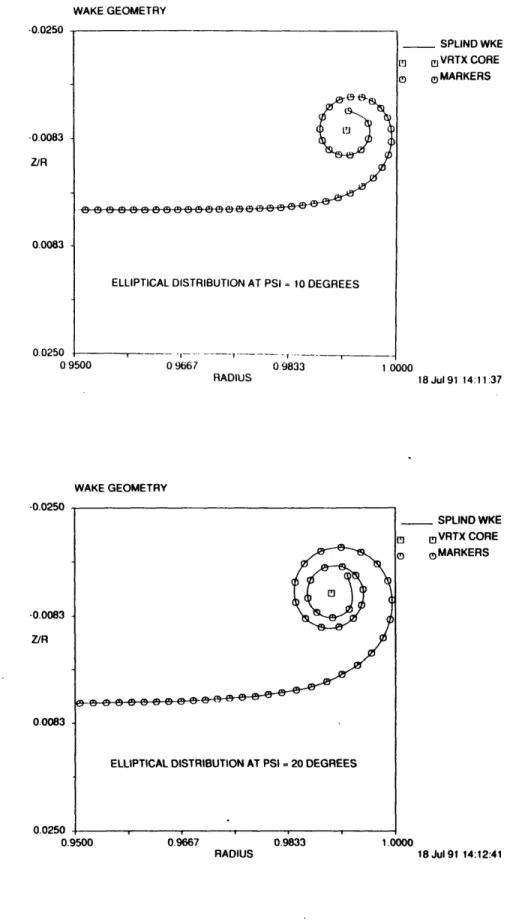
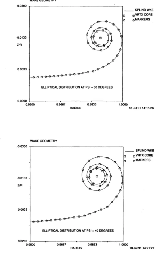
In Figures 4.4-1, 4.4-2, and 4.4-3 the wake is shown convecting downstream as the blade moves from 0 to 45 degrees. As expected, the tip vortex convects downstream slower than the rest of the vortex sheet. There is a significant roll-up in the near-wake, but the vortex remains well-behaved (assisted by the smoothing routine). Only the tip is shown in the following figures since the wake remains relatively flat inboard.

WAKE GEOMETRY -0.U0230 -0.0083 Z/R 0.0083 0.0250 0 9667 0 9833 RADIUS 1 0000 SPLIND WKE ElVRTX CORE 0 MARKERS 18 Jul 91 14:11:37 WAKE GEOMETRY 0.9667 0.9833 RADIUS 1.0000 SPLIND WKE JVRTX CORE 5MARKERS 18 Jul91 14:12:41

Figure 4.4-1 Wake Profiles for the Elliptically Loaded Blade ELLIPTICAL DISTRIBUTION AT PSI - 10 DEGREES

0.9500 -0.0250 -0.0083 Z/R 0.0083 0.0250 0.9500 ^ ^^'^

WAKE GEOMETRY 0.9667 0.9833 RADIUS SPLIND WKE o VRTX CORE COMARKERS 1.0000 18 Jul91 14:15:26 WAKE GEOMETRY SPLIND WKE mVRTX CORE C)MARKERS 18 Jul 91 14:21:27

Figure 4.4-2 Wake Profiles for the Elliptically Loaded Blade

-U.U3U -U.UJUU -0.0133 Z/R 0.0033 0.0200 0.9500 uu nun -U.UJU -0.013 Z/R 0.003 0.020 RADIUS

WAKE GEOMETRY SPLIND WKE J VRTX CORE 0 OMARKERS 18 Jul 91 14:18:25 1.000 WAKE GEOMETRY 0.9667 0.9833 RADIUS 1.0000 SPLIND WKE I VRTX CORE .(MARKERS 18 Jul 91 14:16:59

Figure 4.4-3 Wake Profile for the Elliptically Loaded Blade at T = 450

-0.075

-0.025 Z/R

0.025

0.075

ELLIPTICAL DISTRIBUTION AT PSI = 45 DEGREES

0.850 0.900 RADIUS 0.950 -0.0300 -0.0133 Z/R 0.0033 0.0200 0.9500 .

If the sheet is allowed to convect further downstream, the extent of roll-up may lead to instabilities which could be handled using a dumping technique outlined by Hoeijmakers.15 Using this approach, the vortex sheet is only allowed four revolutions, and any vorticity past that point is fed into the vortex core. The core is then re-located to preserve the center of vorticity. The amount of roll-up is checked at each iteration and the process is repeated.

5. Translating Circular Disk

As a check case, a circulation distribution was developed for an oblate ellipsoid (with minor axis b and major axis a), moving parallel to its axis of rotation b, in the limit as its minor axis goes to zero.16 For this case, an irrotational flow due to a circular disk with radius "a"

results as shown in Figure 5-1. Since the boundary condition states that no flow can pass through this disk, all particles on the disk must descend at the same rate as the disk, producing a constant downwash condition. The intent of this test case is to validate the basic analytic theory developed in this thesis and its application in the present code.

U

I

a

x

Figure 5-1 Oblate Spheroid Collapsed to Circular Disc

2aU

S=D- cosTr

where r and 1 are the elliptical coordinates obtained through the transformation:

x + ia = (a2-b2)1/2sinh(C+il)

For the circular disk, using the coordinate system shown in figure

5-1, it is apparent x and b equal zero while a equals unity. This leaves

the transformation a = sin(iT) , where 0 can be written as:

-2aU

I- (1-02)1/2

The circulation distribution along the plate is simply the change in velocity potential across the plate giving:

-4aU

1(s) = (1-r2)1/ 2

Using this distribution (see figure 5-2), a flat wake exhibiting constant downwash should result. Figure 5-3 shows the resulting downwash distribution for this test case. The circulation distribution was derived assuming a non-dimensional downwash of 0.02 and the code accurately reproduces this value.

CIRCULATION INPUT

0 33 0.67 1.00

CIRCULAT

18 Jul 91 13:29:36

INIT WAKE INPUT

0.00 0.33

R

51--e INIT WAKE

1.00

18 Jul 91 13:34:34

Figure 5-2 Circulation and Wake Distribution for the Oblate Spheroid

0.UUUU0000 0.0100 GAMMA -0.0200 0 0300 0.00 -0.0100 -0.0033 0.0033 0 .0100

INITIAL WAKE INPUT FOR TRANSLATING DISI

I

vindz vs br

0.00 0.33

5-3 Downwash

0.67

Distribution for the Oblate

-0.0400 0.0267 -I veloc vindz -0.0133 0.0000

TRANSLATING DISK RESULTS

Figure 1.00 Spheroid -I -,

Two abnormalities are seen in this plot, one at 80% radius and one at the tip. The slight increase in accuracy seen at .8 radius is due to a higher density of integration strips placed outboard of this location. This is necessary to correctly account for the vorticity in this area where the extent of curvature in the circulation distribution is significantly increased. At the tip spikes are seen on the outer 0.02%. These are due

dr

to the inability of the model handle ss approaching infinity at the tip. 6. Typical Hovering Rotor Loading

The circulation distribution shown in figure 6-1 was chosen as the final test case because there has been considerable debate over the resulting wake geometry. This circulation distribution was obtained iteratively by Miller17 using the entire wake, but has been used in discrete near-wake analyses to try to understand the resulting wake behavior.18 The main point in question is whether or not a mid-span vortex exists. Full-wake discrete models19,20 have shown the formation of a mid-span vortex, however this contradicts experimental results. Since the continuous vortex sheet representation of the present approach is physically more correct, it was hoped that the character of the wake roll-up would more closely match experimental evidence. Figures 6-2 through 6-5 show the roll-up of the wake as the blade advances through 45 degrees.

CIRCULATION INPUT 0.0300 00167 GAMMA 0.0033 -0.0100 0.34 0.67 1.01 18 Jul 91 13:37:42

INIT WAKE INPUT

INIT WAKE VORTEX POS

IIBUTION

18 Jul 91 13:40:29 TYPICAL HOVERING ROTOR CIRULATION I•STI

AFTER SCALED USING PULLIN'S SOLUTION

CIRCULAT TION 0 00 -0.050 -0.017 Z 0.017 0.050 0. ^ ^'^

WAKE GEOMETRY RADIUS 18 Jul 91 14:39:45 WAKE GEOMETRY 1.000 0.933 0.967 RADIUS SPLIND WKE ]VRTX CORE OM A R K E R S 18 Jul 91 14:39:45 = 100 -U. I UU -0.033 Z/R 0.033 0.10( U. IUU SPLIND WKE mVRTX CORE 0MARKERS -0.050 -0.017 Z/R 0.017 0.050 0.900

WAKE GEOMETRY

TYPICAL HOVERING ROTOR DISTRIBUTION PSI = 20 DEGREES 0800 0867 RADIUS 0 933 _ SPLIND WKE w UmVRTX CORE oD MMARKERS 1 000 18 Jul 91 14:45:30 WAKE GEOMETRY 0.933 0.967 RADIUS 1 000 SPLIND WKE EVRTX CORE ®MARKERS 18 Jul 91 15:29:29

Figure 6-3 Wake Profile for Typical Hover Circulation, ' = 200

-0033 Z/R 0.033 0.100 -0.030 0.003 Z/R 0.037 0.070 n ~r\n -U. I VV ---- ~---~---0800 6 0.900

WAKE GEOMETRY 0 100 -0 030 Z/R 0 040 0.110 C_{1800 0.870} IG ROTOR DISTRIBUTION S 0940 1.0 RADIUS SPLIND WKE m mVRTX CORE ( OMARKERS 10 18 Jul 91 14:51:15 WAKE GEOMETRY SPLIND WKE U VRTX CORE MMARKERS 18 Jul 91 14:51:15

Figure 6-4 Wake Profile for Typical Hover Circulation, T = 300

TYPICAL HOVERIN PSI = 30 DEGREE• -0.003 Z/R 0.033 0.070 RADIUS _L~ I i I -- --r-n t0t

WAKE GEOMETRY 0. 100 -0030 Z/R 0.040 0 110 0800 0870 0940 10 RADIUS WAKE GEOMETRY 0.937 0.973 RADIUS 1.010 SPLIND WKE S VRTX CORE ) MARKERS 18 Jul 91 14 54:50

Figure 6-5 Wake Profile for Typical Hover Circulation, I = 450

TYPICAL HOVERING ROTOR DISTRIBUTION PSI = 45 DEGREES -0.020 0.017 Z/R 0.053 0.090 0.900 SPLIND WKE m CIVRTX CORE o( ₀MARKERS 10 18 Jul 91 14:54:50 T

It is seen in figure 6-3, that at T=20 degrees an additional vortex starts to appear. It is induced at approximately 92% blade radius which corresponds with the peak in circulation shown in figure 6-1 (remember only smooth past 96% radius). This roll-up is opposite to that seen at the tip as expected, and becomes more pronounced as the blade convects downstream.

By comparing the elliptical and typical hover circulation distributions, it appears the the outer portion of the wake for the typical hover distribution should convect faster than the elliptical case, and the inner portion slower, which is confirmed by comparing the resulting wake geometries.

8. Conclusions and Future Recommendations

The program resulting from this research can be utilized to assist in resolving the arbitrariness of the finite core size in discrete models, and as the near-wake component of a hovering or forward flight full-wake code.

First, understanding more completely the physical behavior of the near-wake may give insight to why current computer models are not currently matching experimental results.

There seems to be a consensus that representing the wake as a vortex sheet rather than a series of discrete filaments leads to a more realistic model, but at the expense of theoretical and computational

simplicity. Since one methods advantage is the other's weak point, it seems a study comparing the two models would be helpful in determining a fairly simplistic but more physically correct model. It was hoped that a comparison between discrete versus continuous models could be done in this thesis, but was impossible due to the unavailability of a hovering, discrete, near-wake code. By creating a

code similar to the one contained herein (but using a discrete model), a solid analysis could be done. By comparing the results between these

two models, an appropriate core size may become apparent for the discrete model, making its solution much less arbitrary while keeping its simplicity in place.

It does not appear however, that doing this alone will result in the agreement of experimental and computational results, since the more complex continuous model still revealed a mid-span vortex which has yet to be documented experimentally. The reason for this occurrence is still unclear and will possibly only be resolved when viscous terms are included in the wake analysis.

The other primary use for this code, implementation into hovering and forward flight full-wake codes, can be accomplished with minimal changes.

For hovering cases, as outlined in reference 13, the integration

strips are defined as semi-circles from =0 -- to IF=- . By reviewing

equations 3.5, 3.6, and 3.7, it is apparent this modification can be accomplished by simply dividing these equations by 2.