Contactless Voltage and Current Estimation Using
Signal Processing and Machine Learning
by
Alan Casallas
B.S., Massachusetts Institute of Technology (2019)
Submitted to the Department of Electrical Engineering and Computer
Science
in partial fulfillment of the requirements for the degree of
Master of Engineering in Electrical Engineering and Computer Science
at the
MASSACHUSETTS INSTITUTE OF TECHNOLOGY
September 2019
c
○ Alan Casallas, MMXIX. All rights reserved.
The author hereby grants to MIT permission to reproduce and to
distribute publicly paper and electronic copies of this thesis document
in whole or in part in any medium now known or hereafter created.
Author . . . .
Department of Electrical Engineering and Computer Science
August 23, 2019
Certified by . . . .
Jeffrey Lang
Vitesse Professor of Electrical Engineering
Thesis Supervisor
Accepted by . . . .
Katrina LaCurts
Chair, Master of Engineering Thesis Committee
Contactless Voltage and Current Estimation Using Signal
Processing and Machine Learning
by
Alan Casallas
Submitted to the Department of Electrical Engineering and Computer Science on August 23, 2019, in partial fulfillment of the
requirements for the degree of
Master of Engineering in Electrical Engineering and Computer Science
Abstract
This thesis describes a contactless sensor developed to estimate the line currents and line-to-line voltages of a multi-phase cable in the presence of significant external disturbances. The current estimates are derived from an array of point magnetic-field measurements processed by a linear least-square-error estimator. The gains in the estimator are chosen using a probabilistic model of measurement errors created by external magnetic field sources. Test bed validation of the estimates demonstrates estimation errors below 1% even in the presence of nearby cables carrying comparable currents, metal plates that could support eddy currents, and large magnetizable cores. The voltage estimates are derived using actively-guarded electrodes that capacitively couple to the cable conductors. Knowing the coupling capacitance, test bed validation of the estimates again demonstrates estimation errors below 1% even in the presence of nearby cables carrying comparable voltages, and metal plates. A method involving capacitively coupling signals onto the cables is also proposed and demonstrated to determine the coupling capacitance without operator intervention.
Thesis Supervisor: Jeffrey Lang
Acknowledgments
The completion of this thesis would not have been possible without the help of several people and organizations. I would like to thank my thesis supervisor, Professor Jeffrey Lang, for his guidance in developing, testing, and documenting the work in this thesis. Professor Lang was always available to assist me and his vast experience in the field of Electrical Engineering was essential for the success of this research.
I would also like to thank HARTING Corporation for their sponsorship of this research. I would like to thank Vivek Dave for his role as a representative of HART-ING, for facilitating the use of their resources, and for envisioning the future use of the detector produced by this research. I would like to thank Felix Loske, Lutz Troeger, Maren Knop, and Oliver Beyer for maintaining an active interest in the research and for welcoming me during my trip to HARTING facilities in Germany, where the detector was tested on power systems in their production facilities.
I would like to thank Texas Instruments, who were also sponsors of this research. I would like to thank Nevan Clancy Hanumara. Nevan helped us build the light bulb box demo that was presented in the HARTING Business Conference and used extensively for test bed validation.
I would also like to thank the staff at The Cypress Engineering Design Studio at MIT. Dave Lewis and Anthony Pennes were always ready to guide me when assem-bling the PCB board components and 3D printing the yoke.
I would also like to thank Dave Otten for being available when I needed assis-tance with laboratory equipment and with finding the right hardware to use during experiments.
Contents
1 Introduction 25 1.1 Motivations . . . 25 1.2 System Overview . . . 26 1.3 Thesis Goals . . . 28 1.4 Thesis Contributions . . . 29 2 Previous Work 31 2.1 Current Estimation . . . 31 2.2 Voltage Estimation . . . 372.3 Neural Network Methods . . . 40
2.4 Summary . . . 41
3 Hardware and Software 43 3.1 Yoke and PCB Board . . . 43
3.2 Analog-to-Digital Converter . . . 46
3.3 Anti-Aliasing Filter . . . 48
3.4 Test Beds . . . 51
3.4.1 Parallel Cables Test Bed . . . 53
3.4.2 Lightbulb Demo . . . 55
3.5 Software and Data Storage . . . 56
4 Current Estimation Methods 65 4.1 Magnetic Field Sensors . . . 65
4.2 Physics Simulator . . . 66
4.3 Magnetic Field Readings and Interference . . . 68
4.4 The Gain Matrix . . . 72
4.5 Sensor Placement . . . 75
4.6 Error Measurement . . . 81
4.7 Signal Pre-Processing . . . 83
4.7.1 De-Noising Filter . . . 83
4.7.2 Time-Shifting Filter . . . 86
4.7.3 Rogue Frequency Filter . . . 89
4.8 Current Estimation Methods . . . 90
4.8.1 Ordinary Least Squares Estimator . . . 91
4.8.2 Ampere’s Law Estimator . . . 99
4.8.3 Non-linear Model Estimator . . . 103
4.8.4 Linear Model Estimator . . . 106
4.8.5 Spatial Harmonics Estimator . . . 110
4.8.6 BLU Estimator . . . 114
4.9 Machine Learning Methods . . . 125
4.9.1 Regression Estimator . . . 125
4.9.2 Neural Net Training . . . 128
4.9.3 Summary of Current Estimation Methods . . . 131
4.10 Test Bed Validation . . . 133
4.10.1 Parallel Cable Test Bed . . . 133
4.10.2 Lightbulb Demo . . . 137
4.11 Summary . . . 139
5 Voltage Estimation Methods 155 5.1 Coaxial Cable Electrode Sensor . . . 156
5.2 Copper Tape Electrode Sensor . . . 158
5.3 Automatic Calibration . . . 171
5.4 Test Bed Validation . . . 178
5.4.1 Parallel Cable Test Bed . . . 178
5.4.2 Lightbulb Demo . . . 181
5.5 Summary . . . 184
6 Power Estimation 199 6.1 Power Estimates . . . 199
6.1.1 Parallel Cables Test Bed . . . 199
6.1.2 Lightbulb Demo . . . 200
6.2 Summary . . . 201
7 Summary, Conclusions, and Suggestions for Future Work 203
List of Figures
1-1 The system enclosing the three cables consists of a 3D printed yoke, magnetic field sensors (shown in brown), voltage sensors (shown in orange), and PCB boards (shown in green). The sensor signals are col-lected by an Analog-to-Digital converter (ADC) and then transmitted to a laptop for digital processing. The arrows inside the magnetic field sensors indicate their axis of sensitivity. . . 27 2-1 Current sensors using the Hall effect commonly include a circular
mag-netic core, along with an air gap that contains the Hall effect sensor to detect the focused magnetic field. . . 32 2-2 A photo of three HARTING Hall effect current sensors installed around
three cables. The installation of these sensors required an almost full-day shutdown of the electrical system pictured. A single 200 A HART-ING Hall effect sensor can cost $90. Photo courtesy of HARTHART-ING corporation. . . 33 3-1 The first board, which contained eight magnetic field sensors and no
voltage detection hardware. . . 44 3-2 The board glued to the HARTING Han-C Connector, which attached
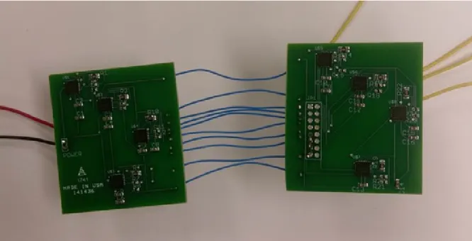
to three 8 AWG cables. . . 44 3-3 The second version of the detector, which contained 12 magnetic field
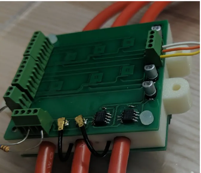
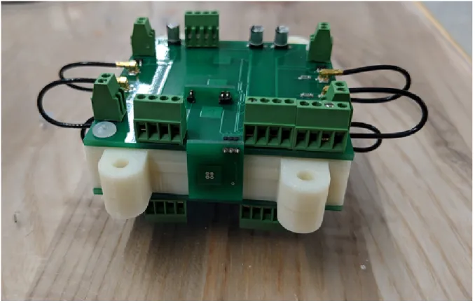
sensors and voltage detection hardware. . . 45 3-4 The third version of the detector, which contains 10 magnetic field
3-5 A CAD model of the top side of a yoke half. The yoke contained indents to fit the magnetic field sensors and terminal block pins so that the PCB board would lay flush on top of the yoke. The yoke also contained four slots for the vertical PCB boards to fit through. . . 47 3-6 A CAD model of the bottom side of the yoke. The three channels that
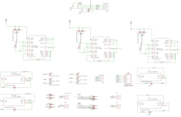
clipped around the cables are visible, as well as smaller channels to fit the coaxial cables that were soldered onto the voltage sensors. . . 48 3-7 An electrical schematic of the main PCB boards. Two of these boards
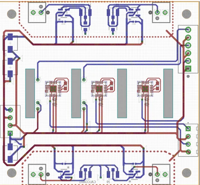
are used in the detector. . . 49 3-8 The board schematic of one of the main PCB boards. Two different
PCB board layouts were required to keep each group of components on the same side when the two boards were attached to the yoke. . . 50 3-9 The board schematic of the other main PCB board., which
comple-ments the boards shown in Figure 3-8. . . 51 3-10 The electrical schematic of a vertical PCB board. Four such boards
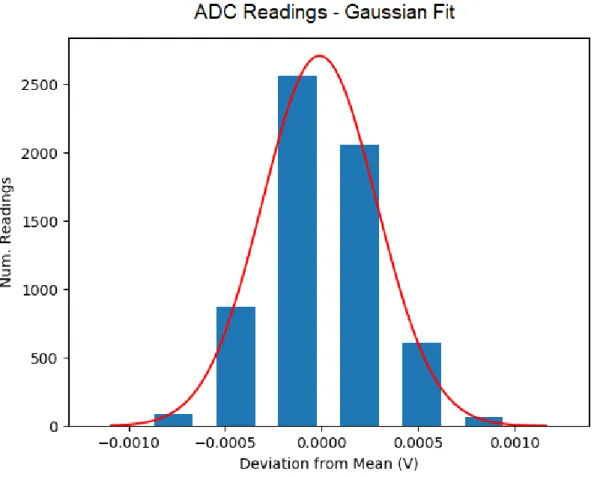
were used in the detector. . . 52 3-11 The board schematic of a vertical PCB board. . . 53 3-12 A histogram of USB-231 ADC readings collected while a constant
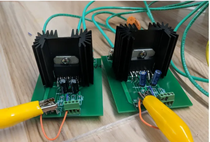
volt-age was applied, with a Gaussian distribution fit over the readings. . 54 3-13 An electrical schematic of the anti-aliasing filter. . . 55 3-14 A photo of the anti-aliasing hardware filter. . . 56 3-15 The parallel cables test bed. . . 57 3-16 The OPA549 power op-amps used to power the parallel cables test bed. 58 3-17 An electrical schematic of the board that housed the OPA549 op-amp. 58 3-18 A schematic of the configuration used to create a balanced set of three
phase currents in the parallel cables test bed. . . 59 3-19 An oscilloscope reading of the voltage output of the two op-amps in
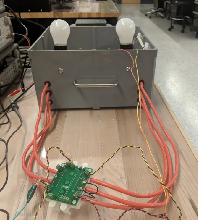
the balanced three phase configuration, showing that they have been tuned to be 120 ∘ out of phase. . . 60 3-20 A photo of the detector attached to the cables of the lightbulb demo. 61
3-21 A schematic of the lightbulb demo. . . 62 3-22 A screenshot of the live display. . . 63 4-1 The final implementation of the magnetic field sensor array placed ten
magnetic field sensors around and between the cables. The sensors are represented as dark rectangles in the figure above. The origin of the coordinate system for the elements in the array is on the left side of the yoke, aligned with the center of the cables. The yoke is 6 cm in width and 1.2 cm in height. Arrows in the magnetic field sensors show their axis of sensitivity. Also shown in this figure are uniform field lines representing one possible orientation of Earth’s magnetic field. The vertical and horizontal decomposition of Earth’s magnetic field, 𝑢𝑥 and 𝑢𝑦, are also shown. . . 67
4-2 Fourier transform of a 2 second sample of magnetic field readings col-lected at 5000 Hz when no current was applied to the cables. . . 70 4-3 Two different gain matrices for the 10 sensor current estimation system.
The values are the gains between the cable currents and the output of the DRV425 sensors, and the units are in V/A. The empirical matrix was obtained by running known currents through one cable at a time using real hardware. The theoretical matrix was generated using the physics simulator. . . 72 4-4 A graph showing the measured output values of a sensor in the sensor
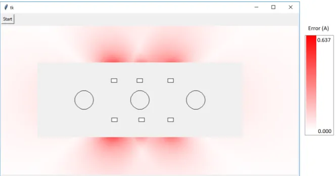
array when known currents were independently run through each cable. 73 4-5 Sensor gains measured as a function of current frequency. . . 74 4-6 A heatmap showing estimation error when the sensors were placed
directly over and under the sensors. The worst case error is 0.177 A. . 77 4-7 A heatmap showing estimation error when two of the sensors were
placed closer to each other. The worst case error is 0.277 A. . . 77 4-8 A heatmap showing estimation error when several sensors have been
4-9 A heatmap showing estimation error when four of the sensors have been placed at the edge of the area in which no external sources of interference can exist. The worst case error is 1.304 A. . . 78 4-10 A heatmap showing estimation error when six sensors are used. This
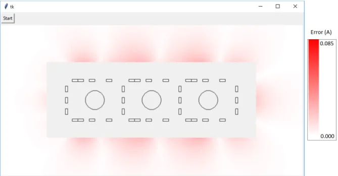
heatmap is similar to the one shown in Figure 4-6, but the color scale has been changed to facilitate comparing this heatmaps with other heatmaps containing different numbers of sensors. The worst case error was 0.189 A. . . 79 4-11 A heatmap showing estimation error when 10 sensors are used. The
worst case error was 0.084 A. . . 79 4-12 A heatmap showing estimation error when thirty-six sensors are used.
The worst case error was 0.025 A. . . 80 4-13 A heatmap showing estimation error when seventy-six sensors are used.
The worst case error was 0.027 A. . . 80 4-14 The true DC current applied to cable, calculated by measuring the
volt-age drop across a 5.08Ω resistor, superimposed over a current estimate for which noise has not been removed. . . 84 4-15 The true DC current applied to a cable, superimposed over an estimate
in which noise has been removed with the Custom Noise Removal filter. 85 4-16 A plot showing readings from the ADC when 2 VPP 130 Hz voltage
was simultaneously applied to all 8 channels. Since the ADC collects readings consecutively, the signals appear out of phase. . . 87 4-17 A plot of the the readings from the ADC when 2 VPP 130 Hz voltage
was simultaneously applied to all 8 channels. The signals have been time shifted, and now correctly appear in phase. . . 88 4-18 Fourier Spectrum showing that different sensors exhibited unique noisy
4-19 A plot showing the Fourier transform of an OLS estimate of 90 Hz current. In this estimate, the gain matrix A was not augmented with uniform field columns, and there is a 60 Hz component visible in the estimate caused by ambient 60 Hz magnetic fields. The readings shown are the voltage output of the DRV425 and thus the magnitude is in volts. 93 4-20 A plot showing the Fourier transform of an OLS estimate of 90 Hz
current formed using a gain matrix A augmented with uniform field columns. The 60 Hz component is largely eliminated from the estimate. The readings shown are the voltage output of the DRV425 and thus the magnitude is in volts. . . 94 4-21 A diagram of the hypothetical scenario. . . 95 4-22 Error contours as a function of distance and current of the external
cable. . . 96 4-23 Estimation error of the simple experiment as a function of the distance
of the external cable. . . 97 4-24 Estimation error using the OLS Estimator as a function of up to 25
sensors. . . 99 4-25 Estimation error using the OLS Estimator as a function of up to 88
sensors. . . 100 4-26 Estimation error using the Ampere’s Law Estimator. . . 102 4-27 An external cable experiment using 3D printed supports. . . 104 4-28 Estimation error of the Linear Model Estimator as a function of the
number of sensors used. . . 107 4-29 Estimation errors as a function of the number of sensors used for the
Second Order Polynomial Estimator. . . 108 4-30 A heat map showing the percent error introduced by an external cable
when the Spatial Harmonics Estimator is used with M=0. . . 111 4-31 A heat map showing the percent error introduced by an external cable
4-32 A heat map showing the percent error introduced by an external cable when the Spatial Harmonics Estimator is used with M=2. . . 112 4-33 A heat map showing the percent error introduced by an external cable
when the Spatial Harmonics Estimator is used with M=3. . . 113 4-34 Estimation error using the Spatial Harmonics Estimator as a function
of the number of sensors. . . 114 4-35 Magnetic fields from an external cable will be detected by the sensor
array in a particular pattern described by the laws of electromagnetism.115 4-36 The numbering of the first 10 sensors used in the physics simulations
involving the BLU estimator. Note the numbering of these sensors is not the same as the numbering of the sensors of the hardware prototype given in Figure 4-1. . . 117 4-37 Estimation error using the BLU Estimator with the first probabilistic
model. . . 119 4-38 Estimation Error using the BLU Estimator with the second
probabilis-tic model. . . 121 4-39 A plot of the voltage output of a particular DRV425 sensor when DC
currents of different magnitudes were run through an external cable. . 122 4-40 A photo of an external cable placed outside the yoke with 3D printed
supports. . . 123 4-41 A photo of an external cable placed underneath the detector. . . 124 4-42 Estimation error using the Regression Estimator as a function of the
number of sensors used. . . 126 4-43 Estimation error using the Regression Estimator with a third degree
polynomial transformation as a function of the nubmer of sensors used. 128 4-44 The training and validation errors of a neural network as a function of
the number of epochs trained. The training set used did not include magnetic field interference. . . 129
4-45 A closer view of the training and validation errors after training for more than 250 epochs for a training set that did not include external
field interference. . . 130
4-46 The training and validation errors of a neural net as a function of the number of epochs trained. The training set used included readings with external magnetic field interference. . . 131
4-47 A closer view of the training and validation errors after 1400 epochs of training on a training set that included external magnetic field inter-ference.. . . 132
4-48 A plot of the voltage data exported by the oscilloscope when 8.3 V 90 Hz voltage was output by the op-amps. . . 134
4-49 The OLS estimate of a set of 1.67 A 90 Hz currents. . . 135
4-50 A plot of the voltage data exported by the oscilloscope when 10 V 90 Hz voltage was output by the oscilloscopes. . . 136
4-51 The OLS estimate of a set of 2 A 90 Hz currents. . . 137
4-52 A pair of external cables were placed 1 cm above the detector. . . 138
4-53 The OLS current estimates. . . 139
4-54 A plate was placed 1 cm above the detector. . . 140
4-55 An experiment in which currents were estimated in the presence of an external plate. . . 141
4-56 The bundle of six cables. . . 142
4-57 An experiment in which current was estimated in the presence of six external cables. . . 143
4-58 An iron core was placed 1.5 cm above the detector. . . 144
4-59 The OLS estimate with 2.79% error. . . 145
4-60 The OLS and the BLU estimators are used to estimate current in the presence of a large iron core. . . 146
4-61 Current estimates when there are no internal currents. . . 147
4-62 The current running through the left light bulb. . . 148
4-64 The current estimate of currents in the light bulb box. . . 150 4-65 Current estimates of the light bulb box in the presence of a pair of
external cables. . . 151 4-66 Current estimates of the light bulb box in the presence of a plate. . . 152 4-67 Current estimates of the light bulb box in the presence of six external
cables. . . 153
5-1 A photograph of the first implementation of our voltage detector. The exposed inner conductor of the coaxial cables can be seen. The red cables are the power cables that carried the voltage being estimated. . 156 5-2 A photograph of the first implementation of our voltage detector. The
exposed inner conductor of the coaxial cables can be seen. The red cables are the power cables that carried the voltage being estimated. . 157 5-3 A plot of estimated and actual voltage in the light bulb box as detected
by the coaxial cable electrodes. The estimated waveform shape lines up well with the actual waveform shape. . . 159 5-4 A graph showing the change in the line-to-line differential electrode
voltage magnitude as a function of time. . . 160 5-5 The electrode consisted of copper tapes taped along each cable
chan-nel of the yoke. Beneath each copper tape is a piece of kapton tape, followed by a second copper tape that served as the active shield. . . 161 5-6 A schematic showing how an op-amp was used to drive the shield to
the same potential as the sensing electrode. Signals 𝑉𝑂𝑢𝑡,1 and 𝑉𝑂𝑢𝑡,2
are read by the ADC. The op-amps are powered by a battery to keep the detector ground separate from the ground of the system being mea-sured. This prevented the calibration signal, discussed in the section on Automatic Calibration, from being shunted. The detector, battery, and ADC all had the same ground. . . 162
5-7 A model of the voltage detection system if the op-amp were ideal. The resistor represents the bypass resistor whose value we chose, and the capacitor models the dielectric effect between the cable voltage and the electrode voltage. . . 164 5-8 A lumped parameter model including the properties of the op amp.
Specifically, the input resistance, gain, and cutoff frequency of the op-amp were modelled. . . 165 5-9 The results of curve fitting the readings to a model that includes
op-amp properties. The measurements were collected using the USB-231 ADC. . . 167 5-10 A graph showing the sensing electrode amplitude as a function of the
cable voltage amplitude. . . 168 5-11 The noisy voltage estimate. . . 169 5-12 Fourier Transform showing large low-frequency voltage estimate
com-ponents. . . 170 5-13 To calibrate the system, we apply a known signal to the calibrating
electrode, represented on the left side of the figure, which capacitively injects a voltage into the cable that then creates a voltage in the sensing electrode. . . 171 5-14 A model showing the full system model of a pair of power cables,
the sensing electrodes, the op-amps driving the active shield, and the calibrating electrodes. If the impedance between the ground of the power cables and the ground of the sensing system is low enough, a shunting path will exist, shown in orange dashed lines, that will greatly reduce the output voltage created by the calibration signal. . . 173 5-15 The lumped parameter model involving the shunt capacitance as well
as the op-amp characteristics. . . 174 5-16 Although the wires used to supply calibration signal were pushed as
far away from the red power cables as possible, they may still have coupled with the cables. . . 178
5-17 Voltage estimates superimposed over a contact measurements. There was no external interference. The error was 0.43% . . . 180 5-18 Voltage estimates of higher magnitude voltage. There was no external
interference. The error was 0.62%. . . 181 5-19 A pair of cables were placed 1.5 cm above the detector. . . 182 5-20 The estimated voltages superimposed over the measured voltages when
two cables were placed above the detector. The voltage estimation error was 0.67%. . . 183 5-21 A plate was placed 1.5 cm above the detector. . . 184 5-22 The estimated voltages superimposed over the measured voltages when
a plate was placed above the detector. The voltage estimation error was 0.68%. . . 185 5-23 A bundle of six cables was placed 1.5 cm above the detector. . . 186 5-24 The estimated voltages superimposed over the measured voltages when
a a bundle of six cables was placed above the detector. The estimation error was 0.62%. . . 187 5-25 Voltage estimates were practically zero when the cables in the detector
were removed. . . 188 5-26 The lightbulb demo voltage. . . 189 5-27 The Fourier transform of the light bulb voltage. The vertical scale is
logarithmic to allow the higher level harmonics to be seen. The custom noise filter described in Section 4.7.1 with a threshold of 0.0008 was applied to the measurements before the logarithmic scale was applied. 190 5-28 The lightbulb demo voltage in the case without interference. . . 191 5-29 A pair of cables was placed 1.5 cm above the detector. . . 192 5-30 The light bulb demo voltage estimate in the presence of interference
5-31 The Fourier transform of the estimated voltage when a pair of cables was placed over the detector. The vertical axis is logarithmic to allow for observation of small signals. The 90 Hz interference created by the external cables can be observed, but it is two orders of magnitude smaller than the main 60 Hz signal. . . 194 5-32 A plate was placed 1.5 cm above the detector. . . 195 5-33 The voltage estimate when a plate was placed above the detector. . . 196 5-34 A bundle of six cables was placed 1.5 cm above the detector. . . 196 5-35 The estimate in the presence of six external cables. . . 197 5-36 The Fourier transform of the estimated voltage when a bundle of six
cables was placed over the detector. The vertical axis is logarithmic to allow for observation of small signals. The 90 Hz interference created by the external cables can be observed, but it is two orders of magnitude smaller than the main 60 Hz signal. . . 198 6-1 The estimated power waveforms in the parallel cables test bed
super-imposed over the measured power waveforms of the test bed. . . 200 6-2 The estimated and measured power waveforms of the lightbulb demo
List of Tables
3.1 Output of anti-aliasing hardware filter. . . 49 3.2 Output of anti-aliasing hardware and software filter. . . 52 4.1 OLS Estimation error in the four test cases. . . 98 4.2 Ampere’s Law Estimation error in the four special cases. . . 102 4.3 Estimation results for an experiment in which two different sets of
initial values were used with the Non-Linear Model Estimator. . . 105 4.4 Estimation results for a second experiment in which two different sets
of initial values were used with the Non-Linear Model Estimator. . . 106 4.5 Linear Model Estimator error in the four special cases. . . 109 4.6 Second Order Polynomial Estimator error in the four special cases. . 109 4.7 Spatial Harmonics Estimator error in the four special cases. . . 113 4.8 BLU Estimator error in the four special cases using the first
proba-bilistic model. . . 119 4.9 BLU Estimator error in the four special cases using the second
proba-bilistic model. . . 121 4.10 First order Regression Estimator error in the four special cases. . . . 126 4.11 Third order Regression Estimator error in the four special cases. . . . 127 5.1 Capacitance between different components of the voltage detector as
measured by an impedance analyzer at 1000 Hz. . . 163 5.2 Comparison of electrode voltage change in the presence of interference
5.3 Electrode voltage when different voltage frequencies were applied di-rectly to the cable. . . 176 5.4 Electrode voltage when different voltage frequencies were applied to
the calibrating electrode while the power cables were disconnected from any load. . . 176 5.5 Comparison of electrode voltage change in the presence of interference
Chapter 1
Introduction
1.1
Motivations
Monitoring cable currents and voltages is a critical task in many commercial and in-dustrial environments, since it can be used to examine the quality and use of electrical power, and track machine health and process performance. However, installing equip-ment to make contact measureequip-ments of current and voltage can be time-consuming and require a lengthy shut down of equipment. For this reason, we have developed a contactless voltage and current sensing system that can be clipped around a set of cables to estimate the current and voltage waveforms within those cables. These es-timates are processed by a computer, which can then perform further digital analysis using the processed waveforms and potentially transmit the data to other computers in a network.
One use for monitoring cable voltage and current is to automatically detect when a machine is failing or encountering trouble. For example, a CNC milling machine executing an automated script can encounter problems if a drill bit cracks or if the script was incorrectly designed and the drill runs into material it cannot cut through. In this case, the machine may start to draw more current as it applies more torque in an effort to complete its task. This increased current draw would be detected by the system we have developed, and since the data can be transmitted via computer networks, an alert can be raised by a central system to inform the operators of the
machine that a problem has occurred. It is even possible to automatically monitor a large number of machines from a central control point.
Another use for monitoring voltage and current is for inferring the state of a machine. For example, a research team at MIT developed a method of estimating the rotor velocity and rotor position of a Permanent-Magnet Synchronous Motor by measuring the current and voltage drawn by the motor by using an observer state space model. [18] Similarly, the state of other machines can be inferred from current and voltage waveforms by using observer state space methods and lumped parameter models. Furthermore, this state information can be used as the feedback component in a control system, effectively enabling sensorless control of machines, such as controlling the position of a motor without the need to install a physical encoder.
Voltage and current information can also be used to diagnose the power quality in a set of a cables. Utility companies will often include terms in their contracts with commercial and industrial customers that penalize injection of harmonics into power lines and require power quality to stay above a certain level. [4] This is because non-linear loads owned by a customer can cause harmonics to appear in power systems, which then propagate back to a utility company’s power lines and create energy losses and extra stress on infrastructure, such as electrical transformers [19]. To deal with this issue, a customer can use the system we have developed to analyze the Fourier components in their cabling and identify when their loads are injecting harmonics into a power system.
1.2
System Overview
The system we developed consists of several components, the implementations of which evolved during the research process:
∙ magnetic field sensors to form current estimates; ∙ electric field sensors to form voltage estimates;
Figure 1-1: The system enclosing the three cables consists of a 3D printed yoke, magnetic field sensors (shown in brown), voltage sensors (shown in orange), and PCB boards (shown in green). The sensor signals are collected by an Analog-to-Digital converter (ADC) and then transmitted to a laptop for digital processing. The arrows inside the magnetic field sensors indicate their axis of sensitivity.
∙ PCB boards to house the electronics and provide electrical connections;
∙ a 3D printed yoke made of two halves that clip around the set of cables;
∙ an Analog-to-Digital Converter (ADC) to convert the analog output of the sensors to digital readings that can be processed by a computer;
∙ a computer to digitally process the readings.
The methods we developed could be used to estimate current and voltage in any number of cables. The system we built is designed to be used with a set of three cables, since a set of balanced three phase cables is commonly found in industrial environments. After digitally processing the sensor readings, the system outputs three current waveforms and two voltage waveforms. The estimated currents are independent of each other; they are not necessarily assumed to be balanced three phase cables. The two estimated voltages are the line-to-line voltages between each pair of cables. In some cases, these waveforms were collected for a one-second or ten-second period and then saved into CSV files. In other cases, they were streamed continuously and displayed in a live graphical user interface. Figure 1-1 shows a sketch of the entire system.
1.3
Thesis Goals
The goal of the thesis was to create a system that could estimate current and voltage waveforms in a set of balanced three-phase cables to within 1% error of the true current and voltage waveforms. These tolerances were chosen because they are comparable to results achieved by commercially available products and the most recent state of the art research. Furthermore, we wished to calculate instantaneous power, power quality, and power harmonics from these measurements. We aimed to estimate current and voltage up to a frequency of 3 kHz, since this is the maximum frequency for which American industrial power customers are usually penalized for harmonic injection. This required a sensing bandwidth of at least 6 kHz. However, we wanted the methods we used to be easily portable to systems requiring much higher bandwidths in the future.
Producing such accurate estimates is a challenging task because of the abundance of nearby interference in industrial environments. Magnetic fields generated from sources other than the cables inside the yoke, such as nearby cables and ferromagnetic materials, can introduce error in a current estimate. Capacitive pickup of external electric fields, coming from sources like nearby electronics and cables, can affect a voltage estimate. Designing a system to reject these disturbances to a tolerance of 1% was a principal novelty of our work.
To deal with external interference in our estimates, we considered two different approaches:
∙ using multiple sensors at different locations and using spatial filtering algorithms to separate the external interference from the internal fields;
∙ using hardware shielding to block out the external fields from reaching our sensors.
In this thesis, we opted to use the first option for current estimation and the latter option for voltage estimation. One reason for this was that the magnetic field shields would be much larger and costlier than the required voltage sensor shields. Another
reason was that this configuration provided the best opportunity to research novel approaches to current and voltage estimation that had not been attempted before and provided promising room for improvement over previous results. Thus, our approach to current estimation involved developing algorithms and software to spatially filter external magnetic fields, while our approach to voltage estimation involved creating the sensor hardware and the shielding mechanism to block external electric fields from reaching the sensors.
1.4
Thesis Contributions
In this thesis we improved on the latest research into current and voltage estimation and we also developed a method to calibrate the capacitance of the electrode used in voltage estimation without operator intervention.
Accurate current estimation of three cable currents using an array of magnetic field sensors in the presence of external magnetic fields has been the topic of several research papers. [12] [17] Many papers examine the use of an Ordinary Least Squares estimator. However, this estimator is not effective in rejecting nearby external in-terference. A more complex estimator was published by researchers at Politecnico di Milano. [24] The research team modelled external magnetic fields as an infinite sum of harmonics and developed a linear estimator that performed better than the Ordinary Least Squares estimator in the presence of a single external cable. The team did not publish results regarding the performance of the estimator in the presence of more challenging interference, such as external plates.
In this thesis we will present a current estimator that offers superior performance to any estimators currently published. The estimator produces estimates with an error of less than 1% in the presence of many different forms of nearby interference. This performance was achieved both by placing sensors in locations that had not previously been considered, as well as by using a probabilistic model of external interference to generate a Best Linear Unbiased estimate. This current estimator, as well as other estimators that we experimented with, is presented in more detail in
Chapter 4.
Accurate voltage estimation in the presence of electric field interference has also been the topic of several research papers. A team at MIT developed a method of using two sensing electrodes at slightly different distances from a cable to increase sensi-tivity to close electric fields and reduce sensisensi-tivity to far away fields. [6] A different research team at La Plata National University developed a voltage sensor that uses a physical shield driven to ground voltage to protect against external interference. [21] However, this shield is only briefly mentioned in the paper and no error percentages are published with regards to its performance.
In this thesis we present a voltage estimator protected by an active shield that is driven to the same voltage as the sensing electrode. We present experiments in which we introduce various forms of interference and demonstrate that the shield enables estimates with less than 1% error in the presence of interference, whereas the error would be significantly greater without the shield. We will present voltage estimation in Chapter 5.
To form accurate voltages measurements without operator intervention, it is also necessary to calculate the capacitance between the cable and the sensing electrode through a calibration scheme. The most successful calibration scheme has been de-veloped by the team at La Plata National University. They report voltage estimates with less than 1% error by use of their calibration method. [20] However, the method requires connecting the detector to the ground of the system being measured, and assumes no significant load between the voltage being measured and the ground of the system.
In this thesis we present a method to calibrate the sensing electrode capacitance without requiring a connection to the ground of the system being measured. In experiments using this method, we estimated the electrode capacitance value with a 30-90% error. However, this is due to limitations of the hardware we used in the detector prototype. A more carefully manufactured detector in which all necessary hardware exists in the form of PCB board components will yield better results using the calibration method we have developed.
Chapter 2
Previous Work
There has been much research into contactless current detection using magnetic field sensor arrays, voltage detection using capacitive sensors, and signal separation tech-niques using machine learning, which can be useful for separating magnetic fields generated by currents from those generated by external sources. We will now present the latest results in these three fields of research.
2.1
Current Estimation
Contactless current estimation is performed by measuring the magnetic fields pro-duced by a current. According to Ampere’s Law, an infinite current-carrying cable will produce a circular magnetic field where the magnitude |𝐵| at a certain point in space is
|𝐵| = 𝜇0𝐼
2𝜋𝑟 (2.1)
where 𝑟 is the distance between the point in space and the center of the cable, 𝐼 is the current magnitude, and 𝜇0 is the permeability of free space. The magnetic field
will have a direction perpendicular to the vector formed from the center of the cable to the point being measured.
One of the most common contactless current sensors today is the Hall Effect current sensor. [19] A Hall effect sensor detects a magnetic field by running an
Figure 2-1: Current sensors using the Hall effect commonly include a circular mag-netic core, along with an air gap that contains the Hall effect sensor to detect the focused magnetic field.
electric current through a semiconductor in such a way that opposing current carriers will be pulled towards opposing sides of the semiconductor by the magnetic Lorentz force. This pulling will create a voltage difference across the width of the conductor, and this voltage difference is measured to determine the magnetic field strength.
Many Hall effect current sensors will include a circular magnetic yoke, used to focus the current-produced magnetic field, with an air gap where the focused magnetic field can be measured by the Hall effect sensor, as shown in Figure 2-1. The magnetic yoke also serves to shield the Hall effect sensor from external magnetic field interference, although this shielding is not perfect and the air gap can be susceptible to interference. [24]
The Hall effect sensor suffers from several shortcomings. Hall effect sensors have a strong dependence on temperature. One study found that the Hall effect voltage changed by as much as 3 mV over a range of temperatures from −40 ∘𝐶 to 125 ∘𝐶 when the magnetic field being measured was kept constant. [26] In fact, although the HARTING HCM open-loop current sensor offers an error of 1% at 25 ∘𝐶, the error rises to 5% at high temperatures. However, HARTING does offer a closed-loop Hall effect sensor that uses a feedback control closed-loop to offer 1% error at higher temperatures, although this sensor draws more power. [14]
Figure 2-2: A photo of three HARTING Hall effect current sensors installed around three cables. The installation of these sensors required an almost full-day shutdown of the electrical system pictured. A single 200 A HARTING Hall effect sensor can cost $90. Photo courtesy of HARTING corporation.
to shield the sensor from external magnetic fields can be large and bulky, such as the one belonging to the HARTING Hall effect sensor pictured in Figure 2-2. A single 900 A Harting Hall effect sensor costs around $90.
Another limitation of the Hall effect sensor is that the properties of the magnetic yoke can limit the frequency of current that can be measured. This can be a limitation if a user is seeking to examine harmonics that exist beyond that range. For example, the open-loop HARTING HCM sensor can detect up to 25 KHz and the closed-loop sensor can detect up to 100 KHz.
There are other types of magnetic field sensors. Magnetoresistive sensors such as AMR and GMR contain materials whose resistance changes with magnetic field. Fluxgate sensors measure magnetic field by using two coils, a drive coil and a sense coil, wound around a ferromagnetic material. A current is run through the drive coil producing an internal magnetic field and driving the material in and out of saturation. The sense coil then detects how much additional magnetic field exists in
the ferromagnetic material from the external surrounding magnetic field. Fluxgate sensors have the advantage of being more accurate, less noisy, and less sensitive to temperature than both Hall effect and magnetoresistive sensors. [16]
Considerable research has been conducted on estimating cable currents without the use of a magnetic yoke core to shield the cable from external fields, due to the high cost and large size of magnetic cores. Such an estimation system involves placing several sensors around a cable to obtain an array of magnetic field point measure-ments. As long as the sensor array is stationary in space, the relationship between magnetic field and current will be linear. This is because the spatial terms in (2.1) will stay constant, so the magnetic field will simply be linearly proportional to the cable current.
One common setup is to design the sensor array such that each sensor is equally distant from the center of the cable and to average the magnetic field values detected by each sensor. [13] Although the accuracy of the current estimate will be affected by errors in the placement of the sensors, the error is not very large. A study into the effect that sensor misplacement had on current estimates found that when 4 sensors were used to estimate current in one cable, a 10 mm lateral offset was needed to introduce a 0.5% error in the estimate and a 25 ∘ rotational offset was needed to introduce a 1% error. The error was even lower when using a larger number of sensors. [13]
Another setup that has been studied extensively is the use of a magnetic field sensor array to estimate the currents in three cables simultaneously. Although the gains between each current and each sensor will be different, they will yield a system of equations that can be used to estimate the currents. If 𝑁 magnetic field sensors are used to detect the magnetic fields produced by 𝑃 currents, a system of 𝑁 equations with 𝑃 unknown variables can be solved to estimate the 𝑃 currents. This system of equations can be represented as a matrix multiplication 𝐴𝐼 = 𝑏, where 𝐼 is a vector of currents, 𝑏 is a vector of magnetic fields, and 𝐴 is a gain matrix. Each component in the matrix 𝐴 is equal to the term 𝜇0𝑐𝑜𝑠(𝜃)
2𝜋𝑟 , where 𝜃 is the angle between the axis of
point being measured. As long as the number of measurements is equal to or greater than the number of unknowns, a current estimate can be derived. Most commonly, Ordinary Least Squares is used to generate a current estimate, given by the formula
ˆ
𝐼 = (𝐴𝑇𝐴)−1𝐴𝑇𝐵. [11]ˆ
Some research projects have focused on the problem of calibrating the gain matrix 𝐴. Although the values of the gain matrix can be theoretically computed, in practice those values may not be known precisely due to sensor or cable misplacement. A power meter developed by a team at MIT attempts to solve this by providing the user with reference loads that can be connected to the cables being measured. [17] These loads draw a predetermined amount of 3 KHz PWM current. This PWM signal can be observed by the sensors and can be used to solve for the gains of the gain matrix. The researchers also developed an algorithm to calibrate the gain matrix without requiring the customer to attach reference loads by instead having the customers power devices already connected to the cables on and off. The algorithm presented in [7] can then calibrate the gain matrix up to a scaling factor. The scaling factor can then be solved for using readings from contact energy meters.
A team at the University of Alberta explored a method to calibrate the gain matrix by solving for the locations of the magnetic field sensors from the magnetic field readings. [12] If the locations of the magnetic field sensors and cables are treated as unknowns, then a system of equations can be formed using the relationship between current and magnetic fields that contains two unknowns for every sensor and cable, specifically, the 𝑥 and 𝑦 location for each element. This model assumes the cables are parallel so that two unknowns are sufficient to describe the location of each element. When enough magnetic field readings are collected from an AC current waveform, there will be more equations than unknowns in the system of equations. Since the system of equations is non-linear, the researchers used a Non-Linear Least Squares (NLLS) solver to solve the equations. An advantage of this method was that since no assumptions are made about the geometry of the cables, it can be used to estimate currents when the three cables are bundled inside a single insulator. Using this method, the team was able to estimate current with an error of 4.63%.
Many research papers have also focused on the challenge of estimating a set of three currents in the presence of external magnetic field interference. In many real-life environments magnetic field sensors will detect not only the magnetic fields created by the currents, but also magnetic fields from other sources, including Earth’s magnetic field, fields from nearby cables, and fields from eddy currents induced in nearby metallic plates. This presents a major challenge that several research teams have made attempts to characterize and solve.
Researchers at Politecnico di Milano approached this problem by characterizing all possible external magnetic fields by a set of linear equations. [24] To do so, they observed that the cross-sectional area containing the three cables would not contain the sources of the magnetic fields that must be filtered out. The sources, such as other cables, are located outside of this area. They then observed that in an area free of magnetic field sources, the magnetic scalar potential at any point will obey Laplace’s Equation, ∇2Φ(𝑟, 𝜑, 𝑡) = 0, and that the solution to this equation can be
expressed as an infinite series known as the circular harmonics of Laplace’s equation. Once the derivative of the magnetic scalar potential is taken, the external magnetic fields can be represented as
𝐻(𝑟, 𝜑, 𝑡) = − 𝑀 ∑︁ 𝑚=1 𝑚𝑟𝑚−1(𝑎𝑚(𝑡)𝑐𝑜𝑠(𝑚𝜑) + 𝑏𝑚(𝑡)𝑠𝑖𝑛(𝑚𝜑))ˆ𝑟 + 𝑀 ∑︁ 𝑚=1 𝑚𝑟𝑚−1(𝑏𝑚(𝑡)𝑐𝑜𝑠(𝑚𝜑) − 𝑎𝑚(𝑡)𝑠𝑖𝑛(𝑚𝜑))ˆ𝜃 (2.2)
where 𝑟 and 𝜑 represent the location of each sensor in polar coordinates, and 𝑀 is the number of harmonics chosen to represent the external fields. Thus, the external magnetic fields are represented as a series of linear equations where the components 𝑎𝑚(𝑡) and 𝑏𝑚(𝑡) are unknown. The total magnetic field detected by each sensor can
be modeled as the sum of the three current-created magnetic fields and the harmonic series above. This leads to a system of equations in which there are 3+2𝑀 unknowns. As long as the number of sensors 𝑁 is equal to or greater than 3 + 2𝑀 , the system of equations can be solved.
The main drawback of this approach is that to fully characterize Laplace’s Equa-tion, an infinite number of linear terms are required. Thus, using a finite number M of components will lead to error in the estimate. However, the researchers conducted simulations that found that this method was effective in reducing the current esti-mation error created by external interference. For example, when an external cable carrying the same current magnitude as the three internal cables was located about 10 cm above the sensor array, the error when using an Ordinary Least Squares esti-mate was around 50%. When using four harmonics the error reduced to around 20% and when using eight harmonics the error reduced to 5%. Note that the results are presented in the form of graphical heatmaps and the values we present are estimates based on the heatmaps presented in the paper.
Several other papers have covered the topic of estimating currents in the presence of interference using an array of magnetic field readings, and have attempted methods similar to the ones described in this section. These papers can be found in [25], [22], [9], [10], [5], and [23].
2.2
Voltage Estimation
Contactless voltage detection can be performed by placing electrodes near cables so that the electrodes capacitively couple with the cable voltages. Since voltage is a differential measurement, in our thesis we focused on measuring line-to-line voltage by using two electrodes to capacitively couple with two adjacent cables.
One of the first contactless voltage detectors was described in 1928. [28] It involved vibrating a plate near a conductor until there was no current running through the plate, which indicated that the plate was vibrating at the same frequency as the voltage in the conductor. The author of this method claims it could measure voltage to 1/1000 volts, although it took several seconds to reach the correct vibrating frequency. More recent voltage detection methods involve electrodes that do not vibrate. A goal of these methods is to measure cable voltage while minimizing the pickup of external electric fields unrelated to the cable voltage. An example of such a system is
one developed by a team at MIT. In this system, two electrodes are placed at slightly different distances from the cable. [15] The two electrodes capacitively couple with the cable voltage with capacitances 𝐶𝑃 1 and 𝐶𝑃 2, and a known resistor and capacitor
are placed between each electrode and ground in parallel. The transfer function between the cable voltage and each electrode is approximately 𝐻(𝑗𝜔) ≈ 𝜔𝑅𝐶𝑃 1 and
𝐻(𝑗𝜔) ≈ 𝜔𝑅𝐶𝑃 2. The capacitances 𝐶𝑃 1 and 𝐶𝑃 2 are inversely proportional to the
distance between the cable and each electrode, such as 𝐶𝑃 1 ∝ 1𝑑. However, rather than
considering the voltage of a single plate, the system considers the differential voltage between the two plate electrodes. The paper shows that since the distance between the two electrodes is much smaller than the distance between the electrodes and the cable, the effective capacitance of the detector, 𝐶𝑃 1− 𝐶𝑃 2, can be approximated to
be inversely proportional to the square of the distance, 𝐶𝑃 1− 𝐶𝑃 2 ∝ 𝑑12. Thus, the
electrode measurement is significantly more sensitive to the cable voltage compared to external disturbances located at far distances.
However, it was not a goal of this MIT research to accurately estimate the magni-tude of the cable voltage. Thus, no attempt was made develop a technique that could calibrate the electrode capacitance 𝐶𝑃, which can vary depending on cable insulation
material. Rather, the designers of the system focused on examining the spectral com-ponents of the voltage and were more interested in the relative magnitudes between frequencies. The resulting system exhibited an error of up to 11.2%, but produced digital waveform estimates that allowed for the relative analysis of the voltage Fourier spectrum. Furthermore, the use of two plate electrodes was effective in mitigating the effect of external electric fields. In one experiment, a fan was suddenly turned on 30 cm from the voltage detection system. Although the estimated voltage initially spiked due to the strong inductive effect of the fan being turned on, the effects of the fan on the voltage estimate dissipated after two line cycles.
Other voltage detection systems have been developed with the goal of accurately estimating cable voltage magnitudes. A system developed at Prince of Songkla Uni-versity uses a copper film wrapped around a cable to serve as an electrode to capac-itively couple with the cable voltage. [27] The researchers manually measured the
electrode capacitance using an LCR meter and found it to be 7.55 pF. They then used a lumped parameter model of their system to estimate the cable voltage and achieved a 2.5% estimation error.
However, the researchers recognized that a major drawback of their system is that the capacitance between the electrode and cable are unknown for different types of cable insulation. Thus, the team has proposed attaching a second electrode to the cable and applying a known voltage to the second electrode. This known voltage will create a capacitively coupled voltage in the cable, which will then be detected by the sensing electrode. If the two electrodes have the same capacitance, the voltage in the sensing electrode can be used to solve for the capacitance of both electrodes. [15] However, this method was only briefly proposed as something that the team would explore and as of this writing has not yet been developed.
Another contactless voltage measurement system has been developed at La Plata National University in Argentina. In this system, a sensing electrode is also used but is driven by a reference voltage. Since the cable voltage and the sensing electrode are at different voltages, a current will flow out of the sensing electrode. This current is processed by an op-amp and a small analog circuit before being digitally processed and used to estimate the cable voltage. [21]
The reference voltage is used to calibrate the system by determining the capac-itance 𝐶𝑋 between the cable conductor and the sensing electrode. The researchers
developed a lumped parameter model of their voltage detection circuit which not only includes the capacitance 𝐶𝑋, but also the capacitance between the op-amp input and
ground, 𝐶𝐼𝑁. According to their model, the output voltage of the detection system is
related to the cable voltage 𝑉𝑋 and reference voltage 𝑉𝑅𝐸𝐹 by the transfer function
𝑉𝑂(𝑠) = −[𝑉𝑋(𝑠) − 𝑉𝑅𝐸𝐹(𝑠)]𝑠𝐶𝑋𝑅 + 𝑉𝑅𝐸𝐹𝑠𝐶𝐼𝑁𝑅 (2.3)
where 𝑅 is the value of a known resistor placed between the sensing electrode and ground.
perform this calibration, the researchers developed a two step process. In the first step, the detector was disconnected from the power cable so that the output voltage would only be related to the reference voltage by 𝑉𝑂(𝑠) = 𝑉𝑅𝐸𝐹𝑠𝐶𝐼𝑁𝑅. This allows
for the value of 𝐶𝐼𝑁 to be determined. In the second step, the detection system is
attached to the power cable, and the reference voltage is run at a different frequency than the cable voltage. Thus, the cable voltage and the reference voltage contributions to the output voltage are distinguishable, and the value of 𝐶𝑋 can be solved.
The latest validation tests run by the researchers achieved an error of 0.7%, which is an improvement over a previous publication of this system which reported errors greater than 2%. Also of note is that this system uses a shield around the electrode driven by the reference voltage to protect against pickup from external electric field sources, although no experimental data is presented to demonstrate the effectiveness of the shield.
A potential concern with this system is that the calibration scheme requires a connection to the ground of the system being measured. The lumped parameter model assumes that the reference voltage is applied with respect to the system ground. However, in some cases it may not be possible to access the ground of the system being measured or there may be a significant and unknown impedance between the cable voltage and the ground.
2.3
Neural Network Methods
The use of neural networks to separate interference from time signals has also been demonstrated. A team at the University of Surrey trained a neural network to sepa-rate vocal audio from song tracks consisting of a mixture of vocal and instrumental audio. [2] Separating human vocal sounds from background noise is referred to as the cocktail party problem.
The research team trained a fully connected neural network of 20500x20500x20500 units. The training samples consisted of 20 second-long segments of music recorded at 44.1 kHz. Each training sample contained the mixed audio consisting of both
vocals and instrumentals, as well as the corresponding recording of vocal-only audio. Sigmoid activation functions were used. The neural network was trained over 100 epochs of training data.
The neural network was successful in separating vocal audio from song tracks. The research team compared the performance of the neural network to Non-negative Matrix Fatorization (NMF), a traditional linear method used for audio signal separa-tion. The neural network performed better than NMF. To quantify their results, the team compared the signal-to-artifact (SAR) ratio to the signal-to-interference (SIR) ratio of the processed tracks. These are two commonly used metrics when evaluating signal separation algorithms. When mean SAR was plotted as a function of mean SIR, the tracks separated using neural networks achieved a score 2.5 dB better than tracks separated using NMF. The team credits the non-linear nature of the neural network for its superior performance compared to NMF, since it allowed the network to identify non-linear relationships between the vocal audio and the mixed audio.
2.4
Summary
The research presented in this section constitutes the most advanced current and voltage estimation techniques published before the research that we will present in the following chapters. In our research, we perform current estimation by using an array of fluxgate magnetic field sensors. We chose fluxgate sensors due to their insensitivity to temperature change, their low cost, the accuracy of their readings, and the low noise level of their readings. We also do not use a magnetic core or any type of magnetic shielding in our detector so as to avoid the weight, size, and cost of such shielding. The focus of our research in current estimation was accuracy in the presence of external interference. The team at Politecnico di Milano has also focused on this task, and approached the problem by orienting all the magnetic field sensors in their array horizontally and by using a harmonic expansion of a physical model of external interference to perform their estimates. [24] In contrast, we not only place magnetic field sensors above and below the cables being estimated, but
also in between and to the sides of the cables, which are locations we did not see considered in any of the papers we reviewed. Additionally, we position the sensors in two different perpendicular orientations, which is a technique we also did not see in any published paper. Furthermore, although all the papers previously discussed used deterministic physical models to estimate currents in the presence of external interference, we use a probabilistic model of external magnetic fields to derive a novel linear least squares current estimator which we will present in Chapter 4.
We perform voltage estimation by using a set of electrodes that capacitively cou-ple with the voltages in the cables. While the papers we presented in this section attempt to estimate the absolute voltage of a cable with respect to the ground of the system being estimated, in our research we are concerned with the line-to-line differ-ential voltage of two adjacent cables. In fact, our voltage detection system is isolated from the ground of the system we are estimating. We also use an active shield to protect the sensing electrodes from external interference. Although the team at La Plata National University uses a shield driven to ground in their detector, they do not present experimental data regarding the performance of their shield. [20] Since re-jecting interference was an important aspect of our work, we collected data regarding its performance and will present it in Chapter 5.
We have also designed a method of calibrating the capacitance between the cable and sensing electrode of the voltage detection system. A calibration system is pre-sented by the team at La Plata National University. [21] However, this calibration scheme requires a connection to the ground of the system being estimated. Further-more, while a system similar to the one we have designed is proposed by the team at Prince of Songkla University, no paper has been published presenting data related to that system. [27]. We have implemented our calibration system and will present the challenges we faced and the estimates we obtained in Chapter 5.
Chapter 3
Hardware and Software
The current and voltage detector consists of several modular components: magnetic field sensors, voltage sensors, PCB boards to house the electronics, a plastic yoke that clips around the cables, analog-to-digital converters to capture the data, anti-aliasing hardware filters, and a laptop to process the readings. The magnetic field sensors and voltage sensors will be described in Chapters 4 and 5. In this chapter, we will describe the other mentioned components.
3.1
Yoke and PCB Board
Over the course of the thesis, we used three different hardware designs for the detector. The first detector, shown in Figure 3-1, used a PCB board that was designed by a group of undergraduate researchers that worked on this project before the start of the thesis. This board contained 8 magnetic field sensors and did not contain any voltage detection hardware. Initially, the detector was envisioned as a clip-on that would attach to the HARTING Han-C connector, an industrial connector that attaches to 8 AWG cables. To prototype the system, we glued the board to the connector as shown in Figure 3-2.
Later we decided the detector should be independent of the HARTING connector and instead designed a 3D-printed ABS plastic yoke that could be clipped around a set of three 8 AWG cables. We also redesigned the PCB board to hold 12 magnetic
Figure 3-1: The first board, which contained eight magnetic field sensors and no voltage detection hardware.
Figure 3-2: The board glued to the HARTING Han-C Connector, which attached to three 8 AWG cables.
field sensors and to house the op-amps used with the voltage detection system. We also included holes to join the board and yoke using nylon screws. An image of this
Figure 3-3: The second version of the detector, which contained 12 magnetic field sensors and voltage detection hardware.
board is seen in Figure 3-3.
Lastly, we designed a third version of the detector, shown in figure 3-4. In addition to six horizontally-oriented magnetic field sensors, this board also contained four vertically-oriented magnetic field sensors to achieve more accurate current estimates, using 90-degree angle pins to electrically connect the magnetic field sensors of different orientations. Furthermore, the voltage detection circuitry was re-arranged to reduce parasitic capacitance.
The 3D-printed plastic yoke was designed using OnShape. CAD drawings of yoke are shown in Figures 3-5 and 3-6. The PCB boards were designed using the Eagle
Figure 3-4: The third version of the detector, which contains 10 magnetic field sensors, including 4 vertically oriented sensors, and voltage hardware.
software. The electrical schematic of both main PCB boards is shown in Figure 3-7. The board schematics of the two PCB boards were different and are shown in Figures 3-8 and 3-9. The electrical schematic of the small PCB boards use to house the vertical sensors is shown in Figure 3-10. The board schematic of the small PCB boards is shown in Figure 3-11.
3.2
Analog-to-Digital Converter
To record voltages and process them into digital form, we used a pair of Analog-to-Digital Converter (ADC) devices by Measurement Computing, the USB-205 and the USB-231. [3] Each device was capable of reading 8 analog inputs from -10 volts to +10 volts.
The USB-205 was a 12-bit device and could represent 212 values between -10 and
Figure 3-5: A CAD model of the top side of a yoke half. The yoke contained indents to fit the magnetic field sensors and terminal block pins so that the PCB board would lay flush on top of the yoke. The yoke also contained four slots for the vertical PCB boards to fit through.
digital readings were 5.11542 mV apart, which is slightly more than 220 𝑉12−1 since the
true range of the device was slightly wider than +/- 10 volts. Likewise, the USB-231 was a 16-bit device and we confirmed all digital readings were 0.32213 mV apart, which is slightly larger than the theoretical value 220 𝑉16−1.
Due to the nature of an ADC, the digital readings were corrupted with a small amount of Gaussian white noise. To characterize this noise, we applied a constant voltage from a signal generator to the ADC, ensuring with a multimeter the voltage was constant to the fifth decimal place. We then plotted a histogram of the collected readings and fit a Gaussian curve to them, such as the one shown in Figure 3-12. We found the standard deviation of the noise in the USB-205 ADC to be 1.50 mV, and the standard deviation of the noise in the USB-231 ADC to be 0.29 mV.
Furthermore, we found the noise behavior was the same regardless of the magni-tude of the applied voltage. Thus, we modeled the signal detected by the ADC as
Figure 3-6: A CAD model of the bottom side of the yoke. The three channels that clipped around the cables are visible, as well as smaller channels to fit the coaxial cables that were soldered onto the voltage sensors.
𝑠[𝑛] = 𝑣[𝑛] + 𝑚[𝑛], where 𝑠[𝑛] is the value recorded by the ADC, 𝑣[𝑛] is the value that would be recorded by an ideal ADC without noise, and 𝑚[𝑛] is a random number taken from a Gaussian distribution.
3.3
Anti-Aliasing Filter
To reduce detection of undesired high frequency signals such as WiFi and Bluetooth, we constructed an anti-aliasing hardware filter. The electrical schematic of this filter is found in Figure 3-13. This filter was implemented as a set of 8 low-pass Sallen-key filters using two 5.1 𝐾Ω resistors, two 0.01 𝜇𝐹 capacitors, and a ua741 op-amp. These values were selected to create a cutoff frequency close to 3000 Hz, since that is the highest frequency we were interested in analyzing in our experiments. A photograph of the filter is shown in Figure 3-14. Table 3.1 shows the gain and phase shift of a series of voltage signals that were applied to the hardware filter as measured by an oscilloscope.
Figure 3-7: An electrical schematic of the main PCB boards. Two of these boards are used in the detector.
Table 3.1: Output of anti-aliasing hardware filter.
Frequency Gain Phase Shift
10 Hz ~1.0 ~0∘ 100 Hz ~1.0 3.5∘ 1000 Hz 0.91 33∘ 2800 Hz 0.57 81∘ 3000 Hz 0.54 86∘ 3200 Hz 0.50 90∘ 5000 Hz 0.29 112∘ 10000 Hz 0.10 139∘
To reduce the effect of the filter on frequencies below 3000 Hz, we developed a digital filter to process the readings output by the hardware filter. The theoretical transfer function of the Sallen-Key filter is
𝐻(𝑗𝜔) = 1
Figure 3-8: The board schematic of one of the main PCB boards. Two different PCB board layouts were required to keep each group of components on the same side when the two boards were attached to the yoke.
The digital filter we created digitally applies the inverse of the above signal by taking the Fourier transform of the input signal, multiplying by the inverse transfer function, and returning the inverse Fourier transform of the result. The filter was implemented in Python. The code of the implementation can be found as the antiantialiasingfilter() function in the file preprocessor.py found in Appendix A.
Table 3.2 shows the gain and phase shift of the signals after passing through the hardware filter and then being processed by the digital filter. The signals were
Figure 3-9: The board schematic of the other main PCB board., which complements the boards shown in Figure 3-8.
sampled by the ADC at 6250 Hz. As the results in the table show, the combination of the both filters was effective in correcting the gain and phase shift of signals under 3000 Hz while attenuating signals above this frequency.
3.4
Test Beds
To validate our detector hardware and algorithms, we built two test bed validation environments that would allow us to control and monitor the true current and voltage
Figure 3-10: The electrical schematic of a vertical PCB board. Four such boards were used in the detector.
Table 3.2: Output of anti-aliasing hardware and software filter.
Frequency Gain Phase Shift
100 Hz 0.999 0.01∘
1000 Hz 1.001 0.20∘
2800 Hz 1.007 0.01∘
3000 Hz 1.007 0.03∘
Figure 3-11: The board schematic of a vertical PCB board.
3.4.1
Parallel Cables Test Bed
The first test bed consisted of three parallel 8 AWG cables connected to two terminal blocks, as shown in Figure 3-15. The terminals in these blocks could be connected in different ways to create a variety of circuit configurations. To control the currents, we used a set of TI OPA549 op-amps that were capable of outputting voltages of +/- 30 V and currents of up to 8 A. They are shown in Figure 3-16. These op-amps allowed us to run low-noise currents at frequencies and amplitudes of our choosing. An electrical schematic of the board that housed each op-amp is shown in Figure 3-17.