HAL Id: hal-01230137
https://hal.archives-ouvertes.fr/hal-01230137
Submitted on 17 Nov 2015
HAL is a multi-disciplinary open access
archive for the deposit and dissemination of
sci-entific research documents, whether they are
pub-lished or not. The documents may come from
teaching and research institutions in France or
abroad, or from public or private research centers.
L’archive ouverte pluridisciplinaire HAL, est
destinée au dépôt et à la diffusion de documents
scientifiques de niveau recherche, publiés ou non,
émanant des établissements d’enseignement et de
recherche français ou étrangers, des laboratoires
publics ou privés.
Suspensions
Juan C. Tudon-Martınez, Soheib Fergani, Olivier Sename, John Jairo
Martinez Molina, Ruben Morales-Menendez, Luc Dugard
To cite this version:
Juan C. Tudon-Martınez, Soheib Fergani, Olivier Sename, John Jairo Martinez Molina, Ruben
Morales-Menendez, et al.. Adaptive Road Profile Estimation in Semi-Active Car Suspensions. IEEE
Transactions on Control Systems Technology, Institute of Electrical and Electronics Engineers, 2015,
23 (6), pp.2293 - 2305. �10.1109/TCST.2015.2413937�. �hal-01230137�
Adaptive Road Profile Estimation
in Semi-Active Car Suspensions
Juan C. Tud´on-Mart´ınez
1, Soheib Fergani
2, Olivier Sename
2,
John J. Martinez
2, Ruben Morales-Menendez
1, and Luc Dugard
2Abstract—The enhancement of the passengers comfort and their safety are part of the constant concerns for car manu-facturers. As a solution, the semi-active damping control systems have emerged to adapt the suspension features, where the road profile is one of the most important factors that determine the automotive vehicle performance. Because direct measurements of the road condition represent expensive solutions and, are susceptible to be contaminated, this paper proposes a novel road profile estimator that offers the essential information (road roughness and its frequency) for the adjustment of the vehicle dynamics by using conventional sensors of cars. Based on the Q-parametrization approach, an adaptive observer estimates the dynamic road signal, posteriorly, a Fourier analysis is used to compute online the road roughness condition and perform an ISO 8608 classification. Experimental results on the rear-left corner of a 1:5 scale vehicle, equipped with Electro-Rheological (ER) dampers, have been used to validate the proposed road profile estimation method. Different ISO road classes evaluate online the performance of the road identification algorithm, whose results show that any road can be identified successfully at least 70% with a false alarm rate lower than 5%; the general accuracy of the road classifier is 95%. A second test with variable vehicle velocity shows the importance of the online frequency estimation to adapt the road estimation algorithm to any driving velocity, in this test the road is correctly estimated 868 of 1,042 m (error of 16.7%). Finally, the adaptability of the parametric road estimator to the semi-activeness property of the ER damper is tested at different damping coefficients.
Index Terms—Road roughness, Semi-active suspension, Electro-rheological damper, Youla-Kuˇcera parametrization.
I. INTRODUCTION
B
ECAUSE of the vehicle dynamics depend on tire/road contact forces and torques, the road profile is one of the most important factors that determine the vehicle performance and the automotive suspension design. The knowledge of the road profile (estimation or measurement) can be used to adapt the damping coefficient on active or semi-active suspension control systems to improve the ride comfort and handling of a car [1]–[4], such as the recent magic body control (look-ahead approach) in luxury cars of Mercedes-BenzTM.On the other hand, because in some cases the road geome-tries, irregularities and deformations are cause of vehicle col-This work is partially supported by the French national project INOVE ANR 2010 BLAN 0308 and by the PCP project 03/2010 (France-M´exico).
1J.C. Tud´on-Mart´ınez and R. Morales-Menendez are with Tecnol´ogico de Monterrey, Av. E. Garza Sada 2501, 64849, Monterrey N.L., M´exico, e-mail: [email protected]
2S. Fergani, O. Sename, J.J. Martinez and L. Dugard are with Gipsa-Lab, 11 rue des math´ematiques, 38402 Grenoble, France, e-mail: [email protected]
Manuscript received Month Day, Year; revised Month Day, Year.
lisions [5], whose associated rate of global mortality is around 2.2% according to the World Health Organisation (2013), car manufacturers use some road information to compute tire/road frictions, normal forces, etc. in order to increase the road holding through an electronic stability control.
Existing methods for estimating the road roughness are based either on visual inspections [2], [6] or on the use of a fully instrumented vehicle that can take direct measurements from road irregularities, e.g. profilographs [7] or profilometers [8]–[10], which commonly are used for road serviceability and road maintenance and are independent of the type of survey vehicle and of the profiling speed; the problem is that both methodologies are extremely expensive to be im-plemented and require a specialized operation, i.e. knowledge for sensors location, signal processing, etc. Moreover, during winter seasons with snowy environments, laser sensors are impractical. To overcome these drawbacks, methods with low cost instrumentation capable to be implemented on a fleet of vehicles have gained importance, e.g. road estimators based on accelerometers that are rugged, easy to mount and process. Recently, [11] proposed a road roughness estimator based on standard vehicle instrumentation (acceleration measurements) easy to implement; however, the road estimation algorithm depends on a specific frequency, i.e. the approach is designed for a constant vehicle velocity and the result is not ensured when the velocity changes. Similarly, a road estimator based on the Fourier transform of the road, at constant vehicle velocity, is proposed in [1]. In [12] the road roughness is estimated at variable velocity by using different standardized roads (ISO 8608), but the ANN-NARX estimator could demand many computational resources for an online estimation; sim-ilarly [13] proposed an ANN for the road profile estimation by using 7 acceleration measurements as input vector, but for achieving a good classification, the vehicle behavior under each ISO road profile must be used in the learning phase. In [14] a sliding mode observer is proposed to estimate the road profile using a vehicle model of 16 degrees-of-freedom, by showing good simulation results; however, the complexity of the model, the extensive measurement vector (12 signals, including the heave, roll, pitch and yaw motions) and the assumption of constant vehicle velocity compromise its real time implementation. A Kalman filter is used to estimate the road input of an augmented Quarter of Vehicle (QoV) state space model in [15]; however, the road inclusion in the state vector is assumed as a quadratic signal and compromises the adaptation to the vehicle velocity, indeed the ISO 8608 establishes that real roads follow a sum of sinusoidal waves.
Also, sophisticated road estimation methods have emerged; for instance, in [16] a road roughness monitoring system is proposed by using a Bayesian estimator that performs at variable velocity but, a priori information of the road is required. A novel approach based on the cross-entropy method that employs Monte Carlo simulations is proposed in [17] to obtain the optimal road profile estimation by using the sprung and unsprung mass accelerations; however this tech-nique is practically impossible to implement for automotive suspension control purposes because the optimum requires too much computing time, e.g. 5 hours to estimate 100 m of road roughness. The use of microphones to measure the tire noise, in addition with acceleration measurements, allows the road profile classification [18]; however, a robustness study is needed because of the susceptibility of signal contaminations, the implementation of this strategy on a fleet of vehicles is imminently compromised.
By using classic and cheap car sensors (accelerometers), in [4] is proposed a road roughness estimator adaptive to the vehicle velocity based on an H∞ robust observer. Although the approach is feasible for a real time implementation, a state-space representation with knowledge on the vehicle parameters is needed. In order to reduce the computing cost and minimize the implementation complexity, in this paper the Youla-Kuˇcera (YK) parametrization approach is used to estimate the road profile by considering an internal model of the disturbance into the observer through adjusting a parameter vector. The parametric adaptive algorithm used to estimate the road profile is inspired on the tracking control proposed to the disturbance rejection [19]–[21]. Once the road disturbance is estimated, an online Fourier analysis allows the road roughness estimation by using a fundamental frequency estimation module. Experimental results on a 1:5 scale vehicle have been used to evaluate the proposed road profile estimation method; for simplicity, a QoV is used as survey case. Several ISO 8608 road profiles, at different vehicle velocities, with diverse Electro-Rheological (ER) damping coefficients validate the feasibility of the proposed road profile estimation method to be implemented on real time.
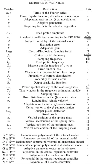
The outline of this paper is as follows: in the next section, the design of the proposed road profile estimator is described. Section III illustrates the experimental-study platform; while the results are discussed in section IV. Concluding remarks are presented in section V. All variables of this study are defined in Table I.
II. ROADPROFILEESTIMATIONALGORITHM Before the decomposition of the road profile signal in frequency and amplitude to determine its roughness level, the estimation of the unknown transient response of the road is performed trough a parametric adaptive algorithm. Posteriorly, an online ISO 8608 road classification is possible by using the Power Spectral Density (PSD) of the estimated roughness.
A. Parametric Adaptive Observation of Road Disturbances
Inspired on a regulation control scheme, it is possible to estimate the road disturbances which theoretically must be
TABLE I DEFINITION OFVARIABLES.
Variable Description Units
α, β Terms of the Fourier series
-δ Dirac impulse function, disturbance model input
-ϵ Adaptation error in the Q-parametrization m
θ Adaptive parameters
λ Forgetting factor in the adaptive algorithm
Azr Road profile amplitude m
cr Roughness coefficient according to the ISO 8608 m
2·m
cycles
d Integer time delay of the internal model
-e Estimation error m
F Adaptation gain
-FER Electro-Rheological damping force N
f0 Critical spatial frequency cyclesm
fs Sampling frequency Hz
fzr Road profile frequency Hz
Gy Discrete transfer function of y vs u
-J Error function cost
-P Characteristic polynomial of closed loop
-Pc Probability of correct classification
-Pf a Probability of false alarms
-Sy Output sensitivity function
-Szr Power spectral density of the road roughness
m2 Hz
Tf Time window in the frequency estimation module s
Ts Sampling time s
u Road disturbances in the Q-parametrization m
vx Longitudinal vehicle velocity ms
w Adaptation vector in the Q-parametrization m
y Output vector in the Q-parametrization m
zdef Damper piston deflection m
zr Road profile m
zs Vertical position of the sprung mass m ¨
zs Vertical acceleration of the sprung mass sm2 zus Vertical position of the unsprung mass m ¨
zus Vertical acceleration of the unsprung mass sm2 A∈ ℜnA Denominator polynomial of the internal model
-B∈ ℜnB Numerator polynomial of the internal model
-D∈ ℜnDDenominator coprime polynomial in disturbance model
-N∈ ℜnN Numerator coprime polynomial in disturbance model
-Q∈ ℜnQ Adaptive parameter vector in the observer
-R0∈ ℜnR Polynomial in the central regulation controller
-R∈ ℜnR Polynomial of a stable controller
-S0∈ ℜnS Polynomial in the central regulation controller
-S∈ ℜnS Polynomial of a stable controller
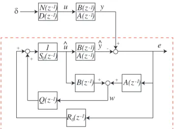
-compensated. This paper makes use of the internal model principle [19] and the YK parametrization (known also as the Q-parametrization) to adjust a parametric vector Q(z−1) that allows the online road estimation. Figure 1 illustrates a block diagram of the adaptive parametric observer using the Q-parametrization approach, the polynomials R0(z−1) and S0(z−1) represent a central controller which respects the reference-servo performances [22].
Because the road profile is deduced from the available car measurements, the observability condition must be guaranteed. In [15] is verified that the QoV model is fully observable when the sprung mass acceleration, suspension deflection or a combination between them is considered as measurement vector; even if the road disturbance model is a sum of sinusoidal waves, the Gilbert observability criterion assures full observability. In this study, the sprung mass position is considered as output vector (y = zs) because has a softer transient response (more damped) than the sprung mass acceleration ¨zs and offers sufficient information for a fully
N(z )
D(z )
B(z )
A(z )
1
S (z )
0 +-A(z )
B(z )
+ +δ
u
y
y^
u
^
e
R (z )
0Q(z )
w
+ + -1 -1 -1 -1B(z )
A(z )
-1 -1 -1 -1 -1 -1 -1Fig. 1. Parametric adaptive observation scheme for road profile disturbances
observable system representation. The discrete-time transfer function of zswith respect to the unknown road input (u = zr) with sampling time Tsis:
Gy(z−1) =
z−dB(z−1)
A(z−1) (1)
where d is an integer time delay in the process (in this case d = 0) and A(z−1) and B(z−1) are polynomials in the complex variable z−1 with orders nA and nB respectively, given by:
A(z−1) = 1 + a1z−1+ a2z−2+ . . . + anAz−n A B(z−1) = b1z−1+ b2z−2+ . . . + bnBz−n
B (2)
By considering a reliable identified model, the central controller is used to specify the desired closed loop poles [22], whose characteristic polynomial is defined by:
P (z−1) = A(z−1)S0(z−1) + z−dB(z−1)R0(z−1) (3) The polynomials S0(z−1) = 1 + s1z−1+ . . . + snSz−n
S and R0(z−1) = r0+ r1z−1+ . . . + rnRz−n
R can be obtained by the Bezout equation as in [20] to obtain a stable solution with minimal pair (S0, R0).
By defining the road disturbance as a deterministic process:
u(k) = N (z
−1)
D(z−1)δ(k) (4)
where δ(k) is a Dirac impulse function and N and D are coprime polynomials of degrees nN and nD, respectively. Based on the internal model principle [19], the transfer func-tion between the road and the vehicle dynamics is given by the output sensitivity function Sy as:
y(k) =S(z −1)A(z−1) P (z−1) | {z } Sy u(k) (5)
In terms of the parametric vector Q, the reference output
y(k) can be defined by: y(k) = S0(z
−1)− z−dB(z−1)Q(z−1)
P (z−1) A(z
−1)u(k) (6)
where S(z−1) = S0(z−1)− z−dB(z−1)Q(z−1) belongs to the family of stable controllers, in the Q-parametrization, that assign the closed loop poles defined by (3). On incorporating the internal model of the disturbance into the polynomial
Q(z−1), is established the diophantine equation [19]:
S0(z−1)− z−dB(z−1)Q(z−1) = S′(z−1)D(z−1) (7) such that,
y(k) =S
′(z−1)A(z−1)N (z−1)
P (z−1) δ(k) (8)
whose unique solution for Q and S′ allows to define a reference output model that implements a perfect disturbance rejection [19]–[21].
For this application problem, the road disturbance is a time-varying signal (in frequency and amplitude) and an adaptation of the internal model is needed to match the actual disturbance. Thus, the adaptation error is given by:
e(k) = y(k)− ˆy(k) (9)
Because y(k) and ˆy(k) can be represented by the
para-metric vector Q(z−1) and ˆQ(z−1) respectively using (6), the adaptation error (9), after some mathematical manipulations, becomes: e(k) = [ Q(z−1)− ˆQ(z−1) ] H(z−1)A(z−1)u(k) (10) where H(z−1) = z−dP (zB(z−1−1)). Because in practice there is no information about the unknown optimal parameter Q(z−1) =
θ0 + θ1z−1 + . . . + θnQz−nQ [20], the adaptation error
ϵ proposed in [19] represents a solution to minimize the
disturbance propagation, such that:
ϵ(k) = S0(z
−1)− z−dB(z−1) ˆQ(z−1)
P (z−1) w(k) (11)
where w(k) represents the effect of the road disturbance into the system output y(k) coming from an output sensor, and it is given by:
w(k) = A(z−1)e(k) + z−dB(z−1)u(k) (12) By expressing the adaptation error ϵ directly in terms of the adaptation coefficients ˆθ, (11) can be rewritten as:
ϵ(k) = S0(z
−1)
P (z−1)w(k)− ˆθ
Tψ(k) (13)
where ψ(k) =[1 z−1 . . . z−nQ]TH(z−1)w(k). By us-ing a gradient algorithm to minimize the error function cost
J = 12ϵ2(ˆθ), the parametric adaptation law is: ˙ˆ
θ = ∂J ∂ ˆθ = ϵ
∂ϵ
∂ ˆθ =−ϵ · ψ (14)
In order to make J small, the adaptation algorithm performs in the direction of the negative gradient with a velocity of adaptation F [20], such that in discrete time the adaptation law becomes:
ˆ
From (12) and applying the YK parameterizacion, the adaptive estimation of the unknown road disturbance [ˆzr(k) = ˆu(k)] is given by:
ˆ u(k) = 1 S0(z−1) ˆQ(z−1)w(k) | {z } θT(k)ϕ(k) +R0(z−1)e(k) (16)
where ϕ(k) = [1 z−1 . . . z−nQ]w(k). The adaptation
gain must be chosen to increase the convergence time of the parameters but with sensitivity to noise around the optimum [22]; generally at the beginning of the algorithm, the gain is enough big and then is decreased. Based on a robust stability analysis with proof in [20], the adaptation gain is given by:
F (k + 1) = λ+ψT(k)F (k)ψ(k)F (k) (17) where λ is the forgetting factor to weight older gain values.
In the narrow-band disturbance rejection problem, the pa-rameter vector ˆθ allows the determination of the disturbance
frequency straightforwardly by fzr = fsarcos(−ˆθ1/2) where fs is the sampling frequency [20], [23], i.e. two coefficients in ˆQ are enough to characterize the frequency of an unknown
sinusoidal disturbance. However, because the road profiles are composed by an indeterminate series of sinusoidal waves, the online estimation of the road frequency through the parameter vector ˆθ is complex. Thus, a frequency estimation module
based on the effective value of the road profile is considered.
B. Road Roughness Estimation and Classification
With the estimations of frequency and amplitude of the road disturbances, it is possible to define the standard type of road profile on which the vehicle is driven.
1) Frequency estimation of the road profile: According to
the ISO 8608, a road profile satisfies a sinusoidal wave whose frequency depends on the vehicle velocity and road quality. Thus, by assuming an harmonic motion in the road, this unknown input could be represented by a sum of sinusoidal waves of the form:
zr(t) ≈ Azr · sin(2π · fzr· t) (18) ˙
zr(t) ≈ 2π · fzr· Azr· cos(2π · fzr· t) (19) where there is no feasible prior information of the road frequency fzr, which depends on: 1) the road surface (number of waveforms), 2) tire dynamics and 3) vehicle velocity. In [24], it is shown that a sum of two or more sinusoidal waveforms with different amplitudes and frequencies can be obtained by the effective RMS value; thus, the road profile frequency can be estimated by the RMS values of the road disturbance computed by (16) and its numerical differentiation
f′(ˆzr), such that: ˆ fzr(k) = √ [f′(ˆzr)2(k)+f′(ˆzr)2(k−1)+···+f′(ˆzr)2(k−n)] [ˆz2 r(k)+ˆz2r(k−1)+···+ˆz2r(k−n)]·4π2 [Hz] (20)
where n is the number of samples in a time window which guarantees at least 2 cycles of the estimated frequency [25].
2) Amplitude estimation of the road profile: By using a
Fourier analysis in discrete time of the estimated road signal (ˆzr) over a running window of one cycle of its fundamental frequency, it is possible to estimate the magnitude of the road by:
ˆ
Azr(k) = √
α2(k) + β2(k) (21)
where the terms of the Fourier series, related to the fundamen-tal component, are:
α(k) = N1 ∑Nn=0−1zˆr(n)cos ( 2π ˆfzrnk ) β(k) = N1 ∑Nn=0−1zˆr(n)sin ( 2π ˆfzrnk ) (22)
The on-line estimated frequency ˆfzr is the fundamental frequency of the road over the running window, i.e. N = 1/ ˆfzr. Thus, the estimations of the frequency and amplitude of the road disturbances are used to monitor its roughness. The roughness Power Spectral Density (PSD) function, Szr(fzr), is used to characterize a road in the frequency domain, [26]:
Szr(fzr) = ˆ
A2
zr
2∆f (23)
where ∆f is defined by the frequency range of interest. By using the limits of roughness for each type of standard road, defined by the ISO 8608, it is performed an online classification of the road on which the vehicle is driven. The thresholds are computed by using the vehicle velocity and the PSD of each road based on the limit of the roughness coefficient (cr) associated with the pavement quality. The lower/upper control limits for each road profile are given by:
SzrT H(fzr) = cr vx · [ fzr (f0·vx) ]−nr [m2/Hz] (24)
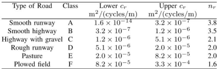
where fzr is the on-line estimated frequency by using (20), f0 is the critical spatial frequency made equal 1/2π cycles/m, vx is the longitudinal vehicle velocity and nr is a dimensionless constant related to the road waves [27]; for disturbances with high wave length (greater than 6 m) nr > 2 [28]. Table II shows the cr coefficient used to define the thresholds of different ISO roads in the road identification algorithm.
TABLE II
CLASSIFICATION OF ROAD PROFILES(ISO 8608).
Type of Road Class Lower cr Upper cr nr m2/(cycles/m) m2/(cycles/m) Smooth runway A 1.6× 10⁻¹⁴ 3.2× 10⁻⁷ 3.8 Smooth highway B 3.2× 10⁻⁷ 1.2× 10⁻⁶ 3.5 Highway with gravel C 1.2× 10⁻⁶ 5.1× 10⁻⁶ 2.1 Rough runway D 5.1× 10⁻⁶ 2.0× 10⁻⁵ 2.0 Pasture E 2.0× 10⁻⁵ 8.2× 10⁻⁵ 2.0 Plowed field F 8.2× 10⁻⁵ 3.3× 10⁻⁴ 1.6
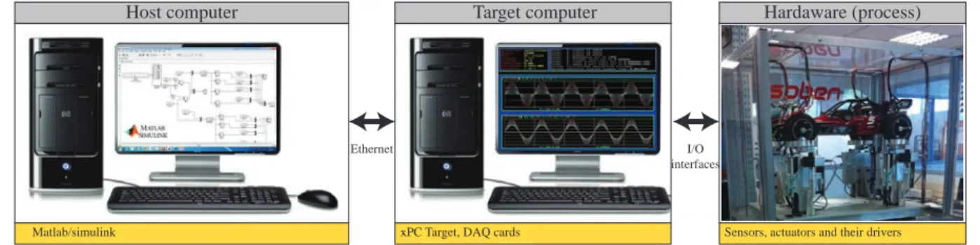
III. EXPERIMENTALSYSTEM:VEHICLE1:5SCALE The experimental platform is composed by a host computer that is used to design and develop the proposed road profile estimation algorithm in Matlab/SimulinkTM. The host com-puter is communicated by a target comcom-puter by ethernet to run the SimulinkTM development in real-time with a xPC Target
Host computer Target computer Hardaware (process)
Matlab/simulink xPC Target, DAQ cards Sensors, actuators and their drivers Ethernet I/O
interfaces
Fig. 2. Experimental platform used to validate the proposed road profile estimation algorithm.
Fig. 3. Experimental vehicle of scale 1:5, developed in the context of the INOVE ANR 2010 BLAN 0308 project.
software of MathworksTM. The target computer also contains a data acquisition card that establishes a bidirectional com-munication with the sensors and actuators of the experimental vehicle. The xPC Target enables control, monitoring, and on-the-spot parameter tuning of the real-time application directly from the SimulinkTM model even if the program is running. Figure 2 shows a conceptual scheme of the used experimental platform; the used sampling frequency was 200 Hz.
An experimental vehicle of scale 1:5, developed by SobenTM in the context of the French national project INOVE ANR 2010 BLAN 0308, is used as test-bed, Fig. 3. The vehicle is equipped with electro-rheological dampers, one at each corner, and is completely instrumented to measure its vertical motion. Each QoV has a DC motor to implement the road profile excitation, whose maximum height is 50 mm and is controlled by a frequency variator.
For simplicity, the road profile estimation algorithm is carried on the rear-left QoV whose available measurements are: road profile zr, unsprung mass position zus, unsprung mass acceleration ¨zus, damping force FER and suspension deflection zdef.
In this experimental implementation, the transfer function
Gy(z−1), eq. (1), which describes the vertical dynamics of the vehicle with respect to (w.r.t.) the road disturbances, is obtained by the ARX model identification given by:
y(k) + a1y(k− 1) + . . . + anAy(k− nA) = b1u(k− d − 1) + . . . + bnBu(k− d − nB) + η(k)
where η(k) is the error between the experimental data and the
model. In the identification process using least squares, y(k) is the sprung mass position obtained from measurements as
zs= zdef+zusand u(k) is the road profile measurement used as reference. Experimental data of different road sequences were used in the identification procedure, by considering a semi-active force at different damping coefficients. Figure 4 illustrates the identification performance of the parametric model Gy(z−1), when the car passes on a road disturbance with soft roughness (type B, ISO 8608) and high roughness (type E, ISO 8608) at the same level of damping force in the
ER shock absorber. 54 56 58 60 62 −0.03 −0.02 −0.01 0 0.01 0.02 0.03 Time [s]
Sprung mass position [m]
experimental data
model
Road E Road B
Fig. 4. Experimental data (solid line) versus the parametric model Gy(z−1) (dashed line). The identified polynomials were: A(z−1) = 1− 4.678z−1+ 8.915z−2−8.648z−3+4.272z−4−0.860z−5and B(z−1) = 0.045z−1− 0.080z−2− 0.013z−3+ 0.091z−4− 0.043z−5.
Figure 5 schematizes the real time validation of the proposed road profile estimation algorithm. The Q-parametrization allows the adaptive estimation of the road disturbance, and posteriorly this signal is used to determine its roughness and perform an ISO road classification.
IV. RESULTS
Different experiments were used to analyze the performance of the proposed road profile estimation strategy. Firstly, re-sults of the Q-parametrization algorithm to estimate the road disturbances are discussed, a forgetting factor λ = 1 was used. Posteriorly, results of the road roughness estimation are presented through a classification analysis.
1 S (z )0 + -A(z ) B(z )+ + y = z y^ u ^ e R (z )0 Q(z ) w + + B(z ) A(z ) -1 -1 -1 -1 -1 -1 -1 Q - parameterization s u = zr ^ Experimental platform Frequency estimation module ^ fz r Discrete Fourier analysis fz r Szr( )
Road roughness estimation
ISO road classification
Experimental ISO 8608 road
Fig. 5. Block diagram to estimate and classify a standardized road profile in real time.
A. Performance of the Parametric Adaptive Observer of Road Disturbances
Test #1: Sinusoidal disturbance, passive car suspension:
In this test, a sinusoidal wave at constant frequency (7 Hz) is considered as road signal, and the automotive suspension system is at passive mode (without actuation). Figure 6a illustrates that the parametric adaptive algorithm allows a very accurate road estimation by using only two parameters in the
Q vector, as it is established in [20], [23]. Indeed, in around
three seconds the parameters achieve their convergence value, Fig. 6b, by using a higher adaptation gain at the beginning of the algorithm which decreases once the Q-parameters values are being adapted, Fig. 6c. Note in Fig. 6a that meanwhile the parameter vector Q is online adapted, the amplitude of the road signal is increasing until achieve the real value (10 cm).
−0.015 −0.01 −0.005 0 0.005 0.01 0.015 Road profile, z [m] r
Experimental data Estimation
−20 0 20 40 60 80 100 Q -parameters values 0 1 2 3 4 5 6 7 8 9 10x 10 8 0 1 2 3 4 5 6 7 8 9 10 Time [s] Adaptation gain F
(a) Estimation performance of the road disturbance
(b) Online adaptation of the Q-parameters
(c) Online adaptation of the gain F
Fig. 6. Road disturbance estimation with Q-parametrization, when zr is a sinusoidal wave at 7 Hz and the car has passive damping suspension.
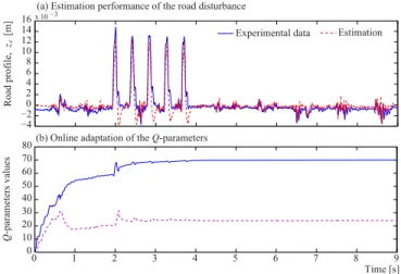
Test #2: Abrupt disturbances, semi-active car suspension:
The road signal is composed by a series of five bumps in this test, which are considered abrupt impulse disturbances. Figure 7a shows that the road is well estimated by the Q-parametrization; only a small overshoot in the negative crests is presented, because the vehicle dynamics (e.g. zs) has this
behavior due to the rebound damping effect. As a sinusoidal wave, two parameters θ are enough in the parametric adaptive algorithm to estimate these kind of disturbances. Figure 7b illustrates that at time when the bumps occur, the parameters are online readapted.
It is important to say that in this case, the sprung mass po-sition zsused in the Q-parametrization, is result of the closed loop transient response of the semi-active suspension control system, e.g. using the classical Sky-Hook control approach. Thus, the controller output does not affect the parametric adaptive algorithm; although the damping coefficient modifies the vehicle dynamics, the transfer function Gy(z−1) between the sprung mass position and the road includes the effect.
Road profile,
z
[m]r Experimental data Estimation
Q
-parameters values
Time [s] (a) Estimation performance of the road disturbance
(b) Online adaptation of the Q-parameters −4 −2 0 2 4 6 8 10 12 14 16x 10 −3 0 1 2 3 4 5 6 7 8 9 0 10 20 30 40 50 60 70 80
Fig. 7. Road disturbance estimation with Q-parametrization, when zr is a series of five bumps and the car has semi-active damping suspension.
Test #3: Road profile disturbances (type D, ISO 8608), semi-active car suspension: In this test, a rough road (type
D according to the ISO 8608) is considered as disturbance to the vehicle dynamics. The car is driven at 30 Km/h, and each 20 s, the damping level is modified by the ER shock-absorber. Figure 8a shows that the suspension deflection movement is inversely proportional to the damping coefficient, i.e. when the damping coefficient in the ER damper decreases, there is a lower energy dissipation and consequently higher suspension motion. However, the disturbance estimation is robust to the damping variation. Figure 8b illustrates that during the 500 m of path at 30 Km/h, the road disturbance is well estimated independently of the damping level in the semi-active suspension system.
of sinusoidal waves, twelve Q-parameters are used in the parametric adaptive algorithm, Fig. 8c. All of them, quickly reach their convergence values (before 3 seconds), using a sufficiently high adaptation gain F as initial value, Fig. 8d, bounded by 2[ψ(k)Tψ(k)]−1[20]. The number of parameters in the vector Q was obtained experimentally because it is completely unknown the number of waves that determine the road profile, their frequency and their contribution to the road roughness. In this study, 12 parameters represent the sum of six sinusoidal waves and the addition of more parameters is not justified by the obtained estimation performance.
Road profile,
z
[m]r
Experimental data Estimation
Q
-parameters values
Time [s]
Adaptation gain
F
(b) Estimation performance of the road disturbance
(c) Online adaptation of the Q-parameters
(d) Online adaptation of the gain F −5 −4 −3 −2 −1 0 1 2 3 4 5x 10 −3 Low damping Medium damping High damping Suspension deflection, z [m] def
(a) Vehicle dynamics at different damping coefficients
−0.02 −0.015 −0.01 −0.005 0 0.005 0.01 0.015 0.02 −50 0 50 100 150 200 0 10 20 30 40 50 60 0 1 2 3 4 5 6 7 8 9 10x 10 8
Fig. 8. Road disturbance estimation with Q-parametrization, when zris an ISO road profile type D, and the car has semi-active suspension at three levels of damping.
On the other hand, considering only two Q-parameters in the adaptive algorithm, it is not possible to represent the road profile disturbance. Figure 9a shows that the estimation result with nQ = 2 is very poor, even the estimated disturbance reaches until 5 cm of height when the real data do not overshoot neither 1.5 cm; also it is possible to see that the estimated signal has more frequency contents than the real one. In contrast, with nQ = 12 the estimated disturbance follows correctly the experimental signal in frequency and amplitude.
Test #4: A random sequence of road profile disturbances (at constant vehicle velocity), semi-active car suspension: This
test allows the evaluation of the Q-parametrization to adapt the disturbance estimation along a random road sequence among different ISO roads. The random sequence has a duration
40 41 42 43 44 45 −0.01 −0.005 0 0.005 0.01 −0.04 −0.03 −0.02 −0.01 0 0.01 0.02 0.03 0.04 0.05 Experimental data Estimation Time [s] (a) Estimation performance of the road disturbance (nQ =2)
Road profile, z [m] r Road profile, z [m]r
(b) Estimation performance of the road disturbance (nQ =12)
Fig. 9. Analysis of performance of the Q-parametrization with two different number of adaptive parameters. The road disturbance to estimate is an ISO road profile type D.
of 260 s at constant vehicle velocity (vx = 30 Km/h), i.e. representing around 2,167 m of path; the suspension system is semi-active at constant damping (without controller). Figure 10a illustrates the road estimation result; the circles show an enlargement of the Q-parametrization performance at different ISO roads, in all cases the estimation follows the experimental road signal, used as reference.
Figure 10b displays the online adaptation of the parameter vector Q. Note in this plot that at the beginning of the adaptive algorithm (during the road type A), the parameters converge almost to the same value; then, all parameters values are adapted again and dispersed when the car passes on a rougher road (type D). Posteriorly, the parameter vector maintains almost constant values because the next roads have less roughness that the road D. When the car is driven on the road E at t = 100 s, the parameters are adapted again with more dispersion and much more even when the road F is present at t = 138 s. From t = 160 to 250 s, the path is less rough than the road F and consequently the current parameter vector Q can estimate correctly these disturbances without a readaptation. Finally, when occurs again the road F, at t = 250 s, the parameters are slightly modified.
B. Road Roughness Estimation
In order to perform the Fourier analysis used in the rough-ness estimation, it is necessary firstly the computing of the road frequency considered as the fundamental frequency in the Fourier series.
With the estimated road disturbance by the
Q-parametrization and its numerical differentiation, the road frequency was estimated by using eq. (20). Figure 11 shows the effect of the time window Tf to compute the discrete RMS values in the frequency estimation module. In this study, a chirp road signal of 5 mm of amplitude with stepped frequency from 1 to 12 Hz was used, Fig. 11a, each frequency has a period of 10 s. Experimentally has been
Experimental data Estimation
Q
-parameters values
Time [s] (b) Online adaptation of the Q-parameters
−0.04 −0.03 −0.02 −0.01 0 0.01 0.02 0.03 0.04
(a) Estimation performance of the road disturbance
Road profile, z [m]r Road E Road C Road F −50 0 50 100 150 200 250 300 350 0 50 100 150 200 250
Fig. 10. Road disturbance estimation with Q-parametrization, when zris a random sequence of different ISO road profiles, and the car goes at constant velocity with medium damping in the ER damper.
validated that a time window of Tf = 1 s, with a sampling frequency of 200 Hz, is the best period to compute the frequency of the road disturbances. Figure 11b displays the estimated frequency with Tf = 0.5 s (100 samples in the time window), note that with this window length, the frequency estimation module has drawbacks to represent frequencies greater than 5 Hz, e.g. the enlargement graph at 11 Hz shows that the estimation does not reach the real frequency, and the signal is not stable; moreover, in some cases the estimated frequency overshoots the real frequency value, as the enlargement graph at 3 Hz. On the other hand, with
Tf = 1 s (200 samples in the time window), the frequency is correctly estimated along the frequency range of interest, Fig. 11c, and it is not necessary to increase the time window size. It is important to say that the addition of time delay caused by the frequency estimation (in this case, 1 s) is negligible for a suspension controller during normal driving over a continuous rough road, such as as an ISO 8608 road.
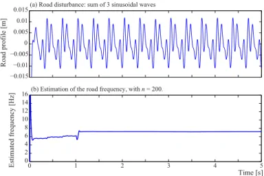
Figure 12 illustrates the capability of the frequency es-timation module to determine the frequency of a sum of sinusoidal waves. In this case, three sine waves compose the road disturbances, which have the same amplitude but different frequency: 3, 8 and 12 Hz. Figure 12b shows that after 1 s (length of time window), the estimated frequency is around the arithmetic average of the three periodic waves. Similar results are obtained when the sine signals have different amplitudes.
With the estimated frequency, the road roughness estimation was performed through a Fourier analysis. In this survey, a classification analysis is used to quantify the performance of the road estimation algorithm in real time. Two experiments with ISO 8608 road profiles were used in this study.
Test #1: Random sequence of ISO road profiles (at constant vehicle velocity), semi-active car suspension: This test
corre-sponds to the test #4 in the Q-parametrization evaluation. By
20 40 60 80 100 120 0 2 4 6 8 10 12 −6 −4 −2 0 2 4 6x 10⁻³ 0 1 Hz 2 Hz 3 Hz 12 Hz T = 1 sf Time [s] Estimated frequency [Hz] Road profile [m] 0 2 4 6 8 10 12 Estimated frequency [Hz] T = 0.5 sf 11 10.8 4 3 11 10.8 4 3
(a) Road disturbance: chirp signal (10 s per frequency)
(b) Estimation of the road frequency, with n = 100.
(c) Estimation of the road frequency, with n = 200.
Fig. 11. Sensitivity of the time window length in the estimation of the road frequency.
Time [s]
Road profile [m]
Estimated frequency [Hz]
(a) Road disturbance: sum of 3 sinusoidal waves
(b) Estimation of the road frequency, with n = 200.
0 1 2 3 4 5 0 2 4 6 8 10 12 14 16 −0.015 −0.01 −0.005 0 0.005 0.01 0.015
Fig. 12. Estimated frequency of a sum of sine waves.
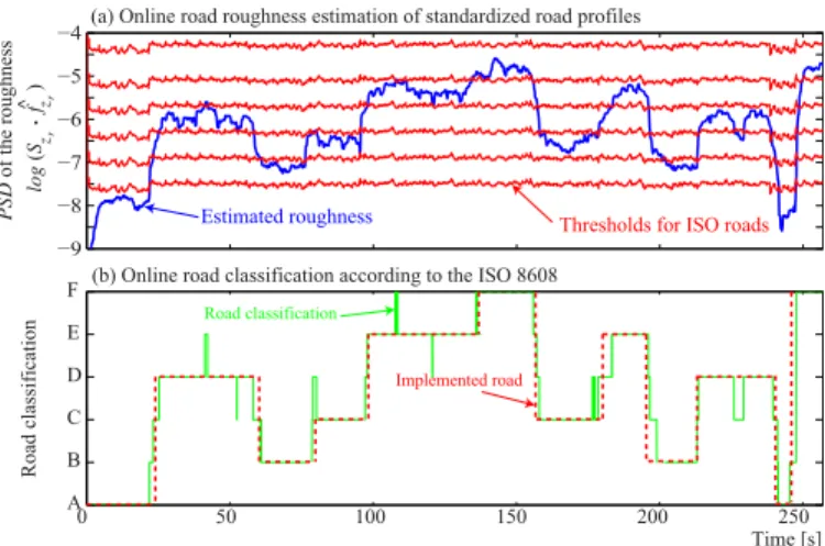
using the estimated road signal, illustrated in Fig. 10a, and its frequency estimation, the on-line road roughness estimation outcome is presented in Fig. 13a by considering the log operator on Szr× ˆfzr; additionally the thresholds SzrT H, which are computed online by using the limits of crfor each road, eq. (24), are used to obtain the road classification result displayed in Fig. 13b. The computation of the PSD road roughness uses the RMS value of ˆAzr(k) in a time window of 1 s in order to have a softer road identification outcome (blue solid line in Fig. 13a).
Figure 13b shows qualitatively that in general, all roads are well classified only with some misclassifications among the neighbors roads. In order to determine a quantitative performance, each road was studied individually by a binary
A B C D E F 0 50 100 150 200 250 PSD
of the roughness log (
S f ) z z r r . Road classification Time [s]
Estimated roughness Thresholds for ISO roads
Road classification
Implemented road
(a) Online road roughness estimation of standardized road profiles
(b) Online road classification according to the ISO 8608 −9 −8 −7 −6 −5 −4 ^
Fig. 13. Online estimation of road roughness, and classification outcome.
classifier system (i.e. a two-class classification problem: posi-tive or negaposi-tive result). Figure 14 illustrates the basic concept of a confusion matrix used to determine the evaluation metrics of the road classifier.
Real condition (Reference)
Condition positive Condition negative FP (Type I error) FN (Type II error) TP TN Positive Negative Test Outcome Sensitivity Pc=TP/(TP + FN) Specificity Pfa=FP/(FP + TN) Positive Precision TP/(TP + FP) Negative Precision TN/(FN + TN) Accuracy (TP+TN)/(P+N)
Fig. 14. Confusion matrix of the test outcome of a classifier.
where, for each road class there exist four classification outcome states:
• True Positive (TP). The road is well classified.
• False positive (FP). It is the error type I, the road is identified in the outcome but experimentally the reference is negative.
• False Negative (FN). It is the error type II, experimentally the road occurs but in the outcome is not identified. • True Negative (TN). The road, correctly, is not classified
because it is not present.
By using these outcome states, it is possible to determine the stronger metrics of a classifier: (1) the sensitivity degree of the classifier for each road, i.e. probability of correct classification
Pc, (2) the specificity degree associated to the probability of false alarm Pf a, and the accuracy degree that quantifies the general performance of the classifier. On plotting the sensitivity vs specificity degree, named Receiver Operating
Characteristic (ROC) curve, it is possible to quantify the
performance of the classifier; the best possible result of classi-fication generates a point in the upper left corner or coordinate (0,1) of the ROC space, representing 100% sensitivity (no false negatives) and 100% specificity (no false positives).
With the use of the confusion matrix, it was determinated
the probability Pc and Pf a for each ISO road profile, and posteriorly it was built the ROC space in the classifier. Figure 15 shows that the classification outcome for all ISO roads was successful, all points are above the diagonal which represents a random outcome. Indeed, the classification outcome for all roads presents a probability of correct classification greater than 70% with minimal false alarm rate (Pf alower than 8%). Table III shows that the accuracy degree of the classifier, in general, is greater than 90% for all road clases, the easier roads to classify are the type A and F.
0 0.1 0.2 0.3 0.4 0.5 0.6 0.7 0.8 0.9 1 0 0.2 0.4 0.6 0.8 1 A B C D E F Probability of classification ( Pc )
Probability of false alarms (Pfa)
Limit of classification
Fig. 15. ROC curve for the classification of ISO 8608 road profiles.
TABLE III
ACCURACY DEGREE OF THE CLASSIFICATION OUTCOME. Road profile
A B C D E F
Accuracy degree (%) 98.7 94.7 90.5 90.8 96.6 99.5
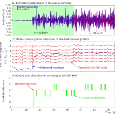
Test #2: Rough road profile at variable vehicle velocity, semi-active car suspension: This test is used to evaluate the
adaptation of the road estimation algorithm to the vehicle velocity. Firstly the car is driven on the road A at low velocity (30 Km/h) and after 15 s, the vehicle passes on the road D at the same velocity; posteriorly, at t = 45 s, a step increment of the vehicle velocity (from 30 to 80 Km/h) is considered keeping the same road class D. Figure 16a shows that at both velocities, the estimation of the road profile through the
Q-parametrization correctly follows the road measurement.
Note in Fig. 16a that when the vehicle is driven at greater velocity, the road frequency is increased but the amplitude is maintained. The online estimation of the PSD road roughness is inside the road type D area independently of the vehicle velocity (30 or 80 Km/h), Fig. 16b. Indeed, the classification outcome in Fig. 16c shows the same misclassification degree from the reference at 30 or 80 Km/h. Figure 17 shows the performance of the classification outcome in this test, the classifier has an accuracy degree of 83.30%, i.e. the road was well classified during 62 of 75 s (868 m of the total path, 1,042 m). The probability of classification is around 78% with a negligible probability of false alarms (Pf a= 0.2%).
The obtained experimental results support the effectiveness of the proposed road profile estimation algorithm, in compar-ison with other published approaches. For instance, in [11] the “simulation” results are highly accurate when the vehicle speed is equal to the used calibration speed in the algorithm; however, the error begins to increase considerably when the
0 10 20 30 40 50 60 70 −8 −7 −6 −5 −4 −3 −2 −0.025 −0.02 −0.015 −0.01 −0.005 0 0.005 0.01 0.015 0.02 0.025 Road profile [m] PSD of the roughness log ( S f ) z z r r . Road identification Time [s] Experimental data
Estimated roughness Thresholds for ISO roads
Road classification Implemented road A B C D E F Estimation v = 30 km/hx v = 80 km/hx
(b) Online road roughness estimation of standardized road profiles
(c) Online road classification according to the ISO 8608 (a) Estimation performance of the road disturbance
^
Fig. 16. Online roughness estimation and classification outcome of the road type D, at variable vehicle velocity.
Reference: road type D
Condition positive Condition negative 7 2699 9301 4197 Positive Negative Test Outcome Sensitivity Pc=0.7750 Specificity Pfa=0.0016 Positive Precision 0.9992 Negative Precision 0.6086 Accuracy 0.8330
Fig. 17. Confusion matrix of the classification outcome of the road type D, at variable vehicle velocity.
vehicle velocity has a difference around 15 Km/h from the calibration speed (which it is considered constant by design). In [1], it is not possible to analyze the performance of the road roughness estimator with clarity due to the absence of the standard roads as thresholds and a random road test; but, 1 second is a good convergence time to estimate the road, as the time window used in the proposed strategy for the road frequency estimation. In [12], the proposed ANN-NARX estimator obtained 10.37% of error with 3 inputs and 15 delays; but, 4,655 s are required to train the model. Therefore, the ANN-based approaches in [12], [13] are impractical for an online estimation of the road roughness used e.g. for control design purposes.
V. CONCLUSIONS
A novel algorithm of road profile estimation and classifi-cation, for semi-active car suspensions, has been proposed. A parametric adaptive observer based on the Youla-Kuˇcera parametrization, also known as Q-parametrization, is used to rebuild the road profile signal by considering an internal
model of this disturbance into the observer through adjusting a parameter vector. The estimated transient response of the road is used to extract its frequency and amplitude in order to compute online the road roughness by performing a Fourier analysis. A road classification algorithm, according to the power spectral density of the road roughness estimation, is used to determine in real time the road on which the car is driven.
The rear-left corner of an experimental car of 1:5 scale has been used to evaluate in real time the proposed approach. Experimental results show that the parametric estimation of the road is adaptive to the damping level in the semi-active shock absorber and, to the roughness level in the road irregularities. The adaptation reaches the optimal Q-parameters in less than 3 s. Also, experimentally it was analyzed the sensitivity of the number of parameters in the Q vector to estimate standardized road disturbances (ISO 8608). A time window of 1 s guarantees the online estimation of the road frequency, which it is considered as the fundamental component in the Fourier series, making to the proposal adaptive to the vehicle velocity.
Two experimental tests have been performed to validate the road roughness estimation. In the first test, a random sequence of 6 different ISO road profiles is used to evaluate the performance of the road estimation algorithm through a classification study. All roads showed a probability of correct identification greater than 70% with minimal false alarm rate (lower than 8%), the general accuracy of the road classifier was 95% (i.e. good estimation during 247 of 260 s). The second test was performed with the same road quality (type D) at two different vehicle velocities (30 and 80 Km/h) to validate the online adaptation of the approach to the vehicle velocity. The road estimation error was 16.7%, this means a good estimation during 62 of 75 s, i.e. 868 m of the total path of 1,042 m.
A future work consists on develop a semi-active suspension controller with online road adaptation, capable to manage the tradeoff between comfort and road holding, and experimen-tally validated on the 1:5 scale car.
REFERENCES
[1] K. Hong, H. Sohn and J. Hedrick, Modified Skyhook Control of
Semi-Active Suspensions: A New Model, Gain Scheduling, and Hardware-in-the-Loop Tuning, ASME Trans. J. of Dynamic Systems, Measurement,
and Control 124 (2002) 158–167.
[2] H. Kim, H. Yang and Y. Park, Improving the Vehicle Performance
with Active Suspension using Road-Sensing Algorithm, Computers &
Structures 80 (2002) 1569–1577.
[3] I. Fialho and G. Balas, Road Adaptive Active Suspension Design Using
Linear Parameter-Varying Gain-Scheduling, IEEE Transactions on
Con-trol Systems Technology 10 (1) (2002) 43–54.
[4] J. Tud´on-Mart´ınez, S. Fergani, S. Varrier, O. Sename, L. Dugard, R. Morales-Menendez and R. Ram´ırez-Mendoza, Road Adaptive
Semi-Active Suspension in an Automotive Vehicle using an LPV Controller,
Proc. of the 7thIFAC Symp. on Advances in Automotive Control, Japan, 2013 pp. 231–236.
[5] F. Aparicio, J. Paez, F. Moreno, F. Jimenez and A. Lopez, Discussion
of a New Adaptive Speed Control System Incorporating the Geometric Characteristics of the Road, Int. J. Vehicle Autonomous Syst. 3 (2005)
47–64.
[6] D. Stavens and S. Thrun, A Self-Supervised Terrain Roughness Estimator
for Off-Road Autonomous Driving, Proc. of the 22thConf. on Uncertainty in Artificial Intelligence (UAI-06), USA, 2006, pp. 469–476.
[7] American Society of Testing and Materials, Standard Test Method for
Measuring Pavement Roughness Using a Profilograph, ASTM E1274,
Annual Book of ASTM Standards, 2008.
[8] E. Spangler and W. Kelly, Profilometer Method for Measuring Road
Profile, General Motors Research, Publication GMR-452, 1964.
[9] A. Healy, E. Nathman and C. Smith, An Analytical and Experimental
Study of Automobile Dynamics with Random Roadway Inputs, J. Dyn.
Sys. Meas. Control Trans. ASME 99 (4) (1977) 284–292.
[10] American Society of Testing and Materials, Standard Test Method
for Measuring the Longitudinal Profile of Traveled Surfaces with an Accelerometer Established Inertial Profiling Reference, ASTM E950-98,
Annual Book of ASTM Standards, 2004.
[11] A. Gonz´alez, E. O ´Brien, Y. Li and K. Cashell, The Use of Vehicle
Acceleration Measurements to Estimate Road Roughness, Vehicle System
Dynamics 46 (6) (2008) 483–499.
[12] H. Ngwangwa, P. Heyns, F. Labuschagne and G. Kululanga,
Recon-struction of Road Defects and Road Roughness Classification using Vehicle Responses with Artificial Neural Networks Simulation, J. of
Terramechanics 47 (2010) 97–111.
[13] M. Yousefzadeh, S. Azadi and A. Soltani, Road Profile Estimation using
Neural Network Algorithm, J. of Mechanical Science and Technology
24 (3) (2010) 743-754.
[14] H. Imine, Y. Delanne and N. M’Sirdi, Road Profile Input Estimation in
Vehicle Dynamics Simulation, Vehicle System Dynamics 44 (4) (2006)
285-303.
[15] W. Yu, X. Zhang, K. Guo, H. Karimi, F. Ma and F. Zheng, Adaptive
Real-time Estimation on Road Disturbances Properties Considering Load Variation via Vehicle Vertical Dynamics, Mathematical Problems in
Engineering 2013 (2013) ID 283528.
[16] T. Heyns, P. Heyns and J. Villiers, A Method for Real-time Condition
Monitoring of Haul Roads Based on Bayesian Parameter Estimation, J.
of Terramechanics 49 (2012) 103–113.
[17] N. Harris, A. Gonz´alez, E. O ´Brien and P. McGetrick, Characterisation
of Pavement Profile Heights using Accelerometer Readings and a Com-binatorial Optimisation Technique, J. of Sound and Vibration 329 (5)
(2010) 497–508.
[18] R. Johnsson and J. Odelius, Methods for Road Texture Estimation using
Vehicle Measurements, Proc. of the 25thInt. Conf on Noise and Vibration Eng., Belgium, 2012 pp. 1573–1582.
[19] I. Landau, A. Constantinescu and D. Rey, Adaptive Narrow Band
Disturbance Rejection Applied to an Active Suspension - An Internal Model Principle Approach, Automatica 41 (4) (2005) 563–574.
[20] J. Martinez and M. Alma, Improving Playability of Blu-ray Disc Drives
by using Adaptive Suppresion of Repetitive Disturbances, Automatica 48
(2012) 638–644.
[21] A. Castellanos-Silva, I. Landau and T. Airimit¸oaie, Direct Adaptive
Rejection of Unknown Time-varying Narrow Band Disturbances Applied to a Benchmark Problem, European J. of Control 19 (2013) 326–336.
[22] I. Landau and G. Zito, Digital Control Systems - Design, Identification
and Implementation, Springer (2005).
[23] T. Airimit¸oaie, A. Castellanos-Silva and I. Landau, Indirect Adaptive
Regulation Strategy for the Attenuation of Time-varying Narrow-Band Disturbances Applied to a Benchmark Problem, European J. of Control
19 (2013) 313–325.
[24] K. Cartwright, Determining the Effective or RMS Voltage of Various
Waveforms Without Calculus, The Tech. Interface 8 (1) (2007) 1–20.
[25] J. Lozoya-Santos, R. Morales-Menendez, O. Sename, L. Dugard, R.A. Ram´ırez-Mendoza and J.C. Tud´on-Mart´ınez, Control Strategies for
an Automotive Suspension with a MR Damper, Proc. of 18thIFAC World Congress, Italy, 2011, pp. 1820–1825.
[26] J. Wong, Theory of Ground Vehicles, John Wiley and Sons, Inc. (2001). [27] J. Robson, Road Surface Description and Vehicle Response, Int. J. Veh.
Des. 1 (1) (1979) 25–35.
[28] G. Genta and L. Morello, The Automotive Chassis: System Design, Springer Science+Business Media (2009).
Juan C. Tud´on-Mart´ınez Obtained the degree of B.Sc. in Chemical Engineering with honors on May 2006 and the M. Sc. degree in Control Engineering on December 2008 from Tecnol´ogico de Monterrey. His research is focused on semi-active suspension control, fault diagnosis and fault tolerant control in vehicle dynamics based on nonlinear control theory and artificial intelligence methods. Actually he is candidate to obtain the PhD degree with dissertation in Fault Tolerant Control in Automotive Semi-Active
Suspensions.
Ruben Morales-Menendez Received the B.Sc. in Chemical Engineering and Systems and two M.Sc. degrees in Process Systems and Automation in 1984, 1986 and 1992, respectively. He has a PhD degree in Artificial Intelligence from Tecnol´ogico de Monter-rey in 2003. From 2000 to 2003, he was a Visiting Scholar with the Laboratory of Computational Intel-ligence at University of British Columbia, Canada. He is a consultant specializing in the analysis and design of automatic control systems for continuous processes for more than 25 years. He is member of the National Researchers System of Mexico (level I), and member of IFAC TC 9.3.