HAL Id: hal-01517087
https://hal.inria.fr/hal-01517087v6
Submitted on 28 Feb 2018
HAL is a multi-disciplinary open access
archive for the deposit and dissemination of
sci-entific research documents, whether they are
pub-lished or not. The documents may come from
L’archive ouverte pluridisciplinaire HAL, est
destinée au dépôt et à la diffusion de documents
scientifiques de niveau recherche, publiés ou non,
émanant des établissements d’enseignement et de
Scalable Machine Learning for Predicting At-Risk
Profiles Upon Hospital Admission
Pierre Genevès, Thomas Calmant, Nabil Layaïda, Marion Lepelley, Svetlana
Artemova, Jean-Luc Bosson
To cite this version:
Pierre Genevès, Thomas Calmant, Nabil Layaïda, Marion Lepelley, Svetlana Artemova, et al.. Scalable
Machine Learning for Predicting At-Risk Profiles Upon Hospital Admission. Big Data Research,
Elsevier, 2018, 12, pp.23-34. �10.1016/j.bdr.2018.02.004�. �hal-01517087v6�
Scalable Machine Learning for Predicting At-Risk
Profiles Upon Hospital Admission
1Pierre Genev`esa,∗, Thomas Calmanta, Nabil Laya¨ıdaa, Marion Lepelleyb, Svetlana Artemovab, Jean-Luc Bossonb
aUniv. Grenoble Alpes, CNRS, Grenoble INP, Inria, LIG, F-38000 Grenoble France bUniv. Grenoble Alpes, CNRS, Public Health department CHU Grenoble Alpes, Grenoble
INP, TIMC-IMAG, 38000 Grenoble, France
Abstract
We show how the analysis of very large amounts of drug prescription data make it possible to detect, on the day of hospital admission, patients at risk of developing complications during their hospital stay. We explore, for the first time, to which extent volume and variety of big prescription data help in constructing predictive models for the automatic detection of at-risk profiles.
Our methodology is designed to validate our claims that: (1) drug prescrip-tion data on the day of admission contain rich informaprescrip-tion about the patient’s situation and perspectives of evolution, and (2) the various perspectives of big medical data (such as veracity, volume, variety) help in extracting this informa-tion. We build binary classification models to identify at-risk patient profiles. We use a distributed architecture to ensure scalability of model construction with large volumes of medical records and clinical data.
We report on practical experiments with real data of millions of patients and hundreds of hospitals. We demonstrate how the fine-grained analysis of such big data can improve the detection of at-risk patients, making it possible to construct more accurate predictive models that significantly benefit from volume and variety, while satisfying important criteria to be deployed in hospitals. Keywords: application, big prescription data, volume, variety, experiments
1. Introduction
A major challenge in healthcare is the prevention of complications and ad-verse effects during hospitalization. A complication is an unfavorable evolution or consequence of a disease, a health condition or a therapy; and an adverse
1This research was partially supported by the ANR project CLEAR (ANR-16-CE25-0010). ∗Corresponding author
Email address: [email protected] (Pierre Genev`es) URL: pierre.geneves.net (Pierre Genev`es)
effect is an undesired harmful effect resulting from a medication or other inter-vention. Typical examples include for instance pressure ulcers, hospital-acquired infections (HAI), admissions in Intensive Care Unit (ICU), and death.
From the perspective of complications, healthcare establishements can be considered as risky environments. For instance, in the USA, an estimated 13.5% of hospitalized Medicare beneficiaries experienced adverse effects dur-ing their hospital stays; and an additional 13.5% experienced temporary harm events during their stays2 [1]. However, physician reviewers determined that
44% of adverse and temporary harm events were clearly or likely preventable [1]. Preventable events are often linked to the lack of patient monitoring and assessment.
One challenging and very interesting goal is to be able to predict the patients’ outcomes and tailor the care that certain patients receive if it is believed that they will do poorly without additional intervention. In doing so, hospitals could prevent unnecessary readmissions, adverse events, or other delays in getting well [2]. For instance, if we can precisely identify groups of patients associated with a very high risk of requiring ICU treatment during their stay, then we can optimize their placement as soon as they are admitted, by affecting them e.g. to rooms closer to ICU, thereby drastically reducing transportation delay in life-critical situations in large hospitals. More generally, many complications could be avoided by immediate identification of at-risk patients upon admission and adapted prevention. A crucial prerequisite to any adapted and meaningful prevention is the precise identification of at-risk profiles.
The widespread adoption of Electronic Health Records (EHR) makes it pos-sible to benefit from quality information provided by healthcare professionals [3]. This opens the way for applying AI techniques in building helpful analytics systems for big medical data in which we can have a high level of trust – since drug prescriptions engage the responsibilities of healthcare professionals.
This paper aims to develop an automatic prediction system for identifying at-risk patients, based on a fine-grained analysis of large volumes of electronic health record data. This has long been viewed as a more challenging task than conventional prediction approaches with summary statistics and EHR-based scores [2, 4].
Contributions.
We show how the analysis of very large amounts of drug prescription data make it possible to detect, on the day of hospital admission, patients at risk of developing complications during their hospital stay. We explore, for the first time, to which extent volume and variety of big prescription data help in constructing predictive models for the automatic detection of at-risk profiles. We report on practical experiments with real data of millions of patients and hundreds of hospitals. We demonstrate how the fine-grained analysis of such big data can improve the detection of at-risk patients, making it possible to
construct more accurate predictive models that significantly benefit from volume and variety, while satisfying important criteria to be deployed in hospitals.
2. Methodology
Our methodology is designed to validate our claims that: (1) drug prescrip-tion data on the day of admission contain rich informaprescrip-tion about the patient’s situation and perspectives of evolution, and (2) the various perspectives of big medical data (such as veracity, volume, variety) help in extracting this informa-tion.
We thus focus on building binary classification models to identify at-risk patient profiles, using distributed supervised machine learning methods. Our approach involves a fully distributed architecture to ensure scalability of model construction with large volumes of medical records and clinical data. The ma-chine learning models that we build yield predictions at hospital admission time. 2.1. Considered Medical Data and Veracity
We consider real data from United States Hospitals. Our dataset features more than 33 million discharges from a representative group of 417 hospitals drawn by lot, as provided by the Premier Perspective database, which is the largest hospital clinical and financial database in the United States. Each in-dividual drug prescription engages the responsibility of the prescriber. Each hospital submits quarterly updates of aggregated data. Patient-level data go through 95 quality assurance and data validation checks. Once the data have been validated, patient-level information is available, comprising data consis-tent with the standard hospital discharge file, demographic and disease state information, and information on all billed services, including date-specific logs of medications, laboratory, diagnostics, and therapeutic services.
The raw data for the year 2006 contains 33 048 852 admissions, and more than three billion patient charge records, representing 2.8 Tb of data.
For our study, we focused on basically two kinds of data: (1) population characteristics (age, gender, marital status, etc.) and (2) clinical data including all drug prescriptions (dosage, route of administration of each drug, etc.) for all admissions.
2.1.1. Filters
We selected adult and adolescent patients (between 15 and 89 years old3),
hospitalized for more than 3 days. We chose this minimal length of stay of 3 days in order to ensure enough time for manifestation and detection of complications during the stay. Other exclusion criteria for the patients were:
3We filtered out other ages because this information was biased in the dataset, i.e. age 89
• patients hospitalized in surgery, because in surgery medical prescription and its complexity varies considerably according to preoperative, opera-tive and postoperaopera-tive phase as described in Lepelley et al. [5] and this information was not available in the dataset);
• out-patients and consultations;
• those with no drug prescription at admission; without which we cannot apply our analysis.
These filters retain 1 487 867 admissions also studied in [5]. We further filter out elective admissions, and finally retain a total of 1 271 733 eligible admissions.
2.1.2. Considered Complications and Ground Truth
To build the complication prediction system, we need labeled data for train-ing and evaluation purposes. We consider four complications:
• death during hospital stay;
• admission to ICU on or after the second day (excluding patients directly admitted to ICU on the first day4);
• pressure ulcers that were not present at admission time but developed during the stay;
• hospital-acquired infections developed during the stay.
Labeling a posteriori the occurrence of deaths and admissions to ICU is trivial as this information can directly be inferred from the medical records. Labeling the occurrence of hospital-acquired infections is slightly more involved since one must basically distinguish secondary infections occurring during hos-pital stay from infections existing before admission. For this purpose, medical experts guided us to label complications in terms of the International Classi-fication of Diseases, Ninth Revision, Clinical ModiClassi-fication (ICD-9-CM) codes [6] that are used in medical records, inspired from the work of Roosan et al. [7]. We implemented complication labeling as a one-pass algorithm that labels each admission with the complication(s) that occurred a posteori (if any). This served to establish a ground truth, which we use for training models.
2.1.3. Participants and Occurrence of Complications
Figure 1 illustrates the distribution of eligible admissions by age and gender. The gap in the number of admissions between genders for people aged between 15 and 40 years is due to pregnancies. The fact that females tend to live longer explains the gap in the number of admissions of older people.
4171 892 people were admitted to ICU on the first day: they have been excluded from the
0
20
40
60
80
0
2500
5000
7500
10000
12500
15000
17500
20000
F
Repartition by Age and Gender
M
Figure 1: Admissions by Age and Gender.
Among the overall population, there were 39 988 cases of hospital death (3.14%), 34 076 cases of pressure ulcers complications (2.68%), 45 542 cases of ICU admission on or after the second day (3.58%), and 32 198 cases of hospital-acquired infections (2.53%). On average, the probability that a patient experiences during his hospital stay at least one of the considered complications is 10.43%.
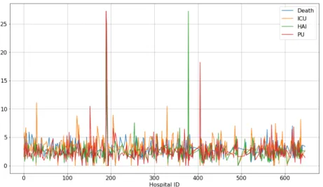
Figure 2 shows the percentage of occurrence of each complication for each of the 417 hospitals considered. The proportion of complications appears roughly
Figure 2: Risk (in %) of Occurrence of Complications per Hospital.
similar between hospitals except for a few of them (shown by the peaks on Figure 2). The filters that we apply (see Section 2.1.1) retain a number of
eligible admissions that varies between hospitals (leaving for instance 15859 relevant admissions for one hospital and 2 relevant admissions for another, with a mean number of 3568 relevant admissions per hospital). The peaks observed on Figure 2 actually correspond to hospitals having a significantly lower number of eligible admissions for our study. For instance, the most important peaks correspond to the following cases:
Death Hospital 189: 49 out of 209 eligible admissions (23.4%) ICU Hospital 29: 95 out of 853 eligible admissions (11.1%) HAI Hospital 378: 6 out of 22 eligible admissions (27.3%) PU Hospital 189: 57 out of 209 eligible admissions (27.3%) We consider that for these cases, the low numbers of eligible admissions explain the peaks observed. In the sequel, we abstract over the fact that some hos-pitals might be more prone to the development of complications than others. We concentrate on developing a predictive system intended to work with any hospital.
Figure 3 illustrates the distribution of drugs served. For each drug (on the x-axis), it shows the (logarithmic) number of patients who were served the drug on their first day. This shows that, as one might expect, some drugs are served to a very large proportion of patients5 while other drugs are rarely served, and
some almost never served. One goal of our predictive system is to automatically extract information from prescription data (including associations of drugs more or less frequently served) relevant for predicting the occurrence of complications. The purpose is to create information and risk signals usable by clinicians. 2.2. Predictive System
We now review the main principles and choices that we have made in de-signing the prediction system.
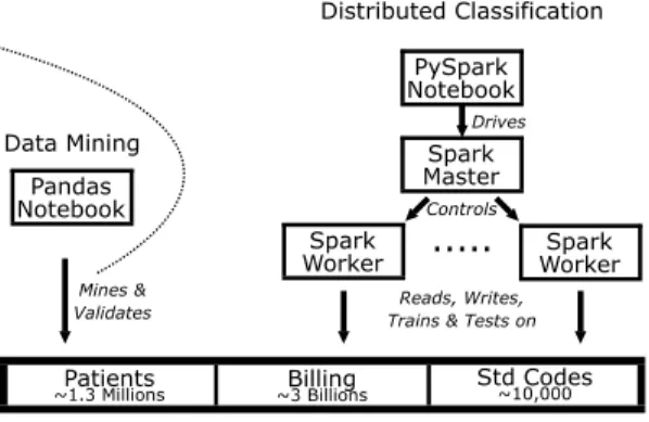
2.2.1. Distributed Approach
Distributing data and computations was instrumental for processing the aforementioned data6. We thus first review the distributed approach that made it possible to obtain our results. The structure of our prediction system is il-lustrated in Fig. 4. Initial data consist in a set of raw relational tables, that we store in a NFS distributed file system. This file system communicates with Spark SQL [8] that we use for data preprocessing, integration, and filtering. For optimizing the representation of features, we use a library for perfect hashing,
5For instance, the top three drugs that are the most served on the first day include
re-spectively “0.9% NACL 1000ML” (served 305 293 times), “PANTOPRAZOLE, PROTONIX TAB 40MG” (served 153 971 times), and “ACETAMIN, TYLENOL TAB 325MG” (served 122 306 times).
6Initial attempts with the Pandas library on a single machine with 160 GB of RAM were
non-conclusive. Only a fraction of the dataset was fitting in memory (after joining and filtering made using a distributed algorithm) and yet no transformation requiring copies (e.g. joins) was possible. We tried to compute joins by chunks and finally stopped the computation after 3 days (for an estimated time of at least 6 days).
0
1000 2000 3000 4000 5000 6000 7000 8000
Drug index
10
010
110
210
310
410
5Occurrences
Figure 3: Distribution of drugs served (the y-axis indicates the number of patients to which each drug on the x-axis was served).
that we modified and upgraded for use in our Spark and Python environments, based on the work of Czech et al. [9]. The feature engineering and classification components are hand coded in Spark [10] and SparkML [11]. We use distributed implementations of Logistic Regression (LR) [12], Linear Support Vector Ma-chines (LSVM) [13], Decision Trees (DT) [14] and FP-Growth [15]. We also used t-SNE [16] and facilities provided by Pandas and Scikit-Learn libraries on smaller excertps of data that were extracted and preprocessed with Spark. We use Docker [17] to improve the runtime performance of the distributed archi-tecture (mainly input/output) compared to a traditional approach with virtual machines. We automatically deploy custom Docker images on each machine of the cluster. The use of Docker also facilitates deployment on commodity and heterogenous machines. We use Jupyter Notebooks as a prototyping frontend.
Our cluster is composed of 5 machines each equipped with 2 Intel(R) Xeon(R) from 1.90GHz to 2.6Ghz, with 24 to 40 cores, and between 60 GB and 160 GB of RAM. The network is 1GB ethernet.
2.2.2. Feature Engineering
The distributed architecture makes it possible to consider many features per patient. We have explored many combination of possible features, going from individual attributes such as the age and gender of a patient, to features describing in more or less details the drugs served on the first day for that patient.
Reads, Writes, Trains & Tests on
Patients
~1.3 Millions ~3 BillionsBilling Std Codes~10,000
PySpark Notebook
Spark Master Spark
Worker ... WorkerSpark
Controls Drives Pandas Notebook Mines & Validates Data Mining Distributed Classification
Figure 4: Architecture of the Prediction System.
For a given patient, we also consider a specific “score” often used in the clin-ical literature and readily available in hospital EHRs: the Medication Regimen Complexity Index (MRCI) [18]. MRCI is one of the most valid and reliable scale for assessing regimen complexity [19]7. The MRCI score is meant to reflect the
complexity of the patient’s situation. The greater the MRCI, the more complex the patient’s situation is. While the minimum MRCI score is 2 (e.g. one tablet taken once a day as needed), there is no maximum score. We retained MRCI as a marker of risk. We also include it in our study for the purpose of comparison with earlier works such as the one of Lepelley et al. [5].
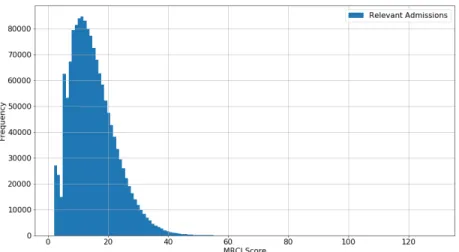
We performed data mining on the dataset and used statistical techniques to search and select basic features among the population characteristics. For example, A 7.9% overall correlation was found between patient’s age and oc-curence of death during hospital stay. Figure 5 illustrates the distribution of MRCI levels among the considered population; and Figure 6 illustrates the per-centage of people who expired at the hospital in terms of their MRCI level at admission. A 4.7% overall correlation was found between the MRCI value at admission and death at the hospital. In the sequel we investigate and report to which extent such correlations can actually be exploited for prediction purposes. We tested different sets of features for building predictive models based on analyses of varying granularity. For the sake of clarity when reporting our
7Specifically, MRCI is a global score aggregating 65 sub-items for the purpose of indicating
the complexity of a prescribed medication regimen. The MRCI has 3 sections giving informa-tion on the dosage form (secinforma-tion A), dosing frequency (secinforma-tion B) and addiinforma-tional instrucinforma-tions (section C) with 32, 23 and 10 items respectively. Each section reflects a different aspect of the complexity of prescription regimen. The total MRCI score is the sum of subscores for the 3 sections. MRCI is readily available in hospital EHRs but for our study, we had to recompute it from our prescription data. We computed it following the Appendix II of [19] which describes how to compute a score for each section. The only approximation is that our considered dataset lacks data required for computing the subscore for section C, which we thus arbitrarily set to zero. In the sequel, the total MRCI score is thus the sum of sections A and B.
Figure 5: MRCI Levels in the Considered Population.
results, we define categories of features and use naming conventions.
For each admission, we concentrate on the following features, grouped by named categories:
• A list B of basic features including patient age, gender, and admission type (e.g. whether the patient is admitted from a doctor’s office and requiring acute care for e.g. pneumonia or dehydration; or whether the patient in life-threatening condition such as accident victim).
• A score M that corresponds to MRCI at admission.
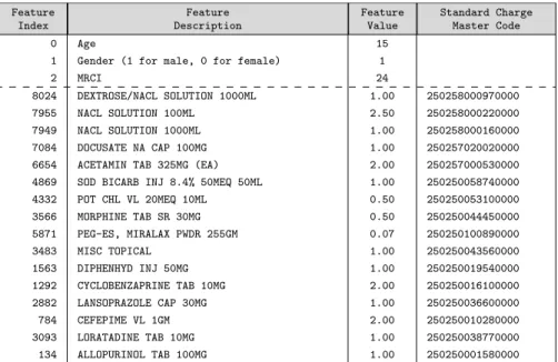
• A list C of clinical quantities associated to drugs prescribed on the first day. The length of C is the number of all drugs possibly prescribed during the first day in any hospital: there are more than 10 thousands such drugs. For example, Table 1 shows a sample vector including clinical quantities of drugs served on the first day. Since only a few drugs are served to each patient on the first day (compared to the length of C), we adopt a sparse representation for features in memory. In addition, we also consider an alternative choice of feature representation where drugs are grouped into drug categories. A drug category regroups drug variants with e.g. different dosage. A category typically regroups 10 drug variants. Thus, as an alternative to the original list C we also consider a list P of integer values (with one integer per category of drugs) indicating the number of drugs served on the first day in the category. Specifically, with our dataset, C contains 10739 entries and P has 2046 entries.
Table 1 illustrates a sample feature vector for a 15 years-old patient, who was served 16 drugs on the day of admission.
We consider combinations of the aforementioned feature categories: for ex-ample B+M, simply denoted as BM, corresponds to the use of all basic features and
0
20
40
60
80
MRCI at admission
0%
20%
40%
60%
80%
100%
Percentage of dead patients
Figure 6: Risk of Death in terms of MRCI Level at Admission.
MRCI; whereas BMC also includes the features corresponding to clinical quanti-ties of drugs served on the first day. In the sequel, we compare the predictive performances achieved with increasingly fine-grained models obtained with BM, BMP and BMC features for instance.
2.2.3. Classifiers
We conducted extensive tests with different classifiers including linear clas-sifiers (LR, LSVM), decision trees and random forests. In the sequel, we mainly report on our experiments with the LR classifier to make predictions. The reason is that LR was the classifier that yielded the best predictive accuracy among several widely-used classifiers (See § 3.1 for comparative metrics and Figures 7 and 8 for comparisons). Notice that LSVM also yields a similar pre-dictive performance. For equivalent performances, we still favor LR because its raw output has a probabilistic interpretation. For our tests, we use the SparkML distributed implementation [11, 10] of the LR classifier [12].
Like several other standard machine learning methods, LR can be formulated as a convex optimization problem, i.e. the task of finding a minimizer of a convex function f that depends on a variable vector w which has d entries. More formally this can be written as the optimization problem
Feature Index Feature Description Feature Value Standard Charge Master Code 0 Age 15
1 Gender (1 for male, 0 for female) 1
2 MRCI 24
8024 DEXTROSE/NACL SOLUTION 1000ML 1.00 250258000970000 7955 NACL SOLUTION 100ML 2.50 250258000220000 7949 NACL SOLUTION 1000ML 1.00 250258000160000 7084 DOCUSATE NA CAP 100MG 1.00 250257020020000 6654 ACETAMIN TAB 325MG (EA) 2.00 250257000530000 4869 SOD BICARB INJ 8.4% 50MEQ 50ML 1.00 250250058740000 4332 POT CHL VL 20MEQ 10ML 0.50 250250053100000 3566 MORPHINE TAB SR 30MG 0.50 250250044450000 5871 PEG-ES, MIRALAX PWDR 255GM 0.07 250250100890000 3483 MISC TOPICAL 1.00 250250043560000 1563 DIPHENHYD INJ 50MG 1.00 250250019540000 1292 CYCLOBENZAPRINE TAB 10MG 2.00 250250016100000 2882 LANSOPRAZOLE CAP 30MG 1.00 250250036600000 784 CEFEPIME VL 1GM 2.00 250250010280000 3093 LORATADINE TAB 10MG 1.00 250250038770000 134 ALLOPURINOL TAB 100MG 1.00 250250001580000
Table 1: Feature vector for a sample patient who was served 16 drugs on the day of admission.
in which the objective function f is of the form:
f (w) = λR(w) + 1 n n X i=1 L(w; xi, yi)
where the vectors xi ∈ Rd are the training data examples, for 1 ≤ i ≤ n, and
yi∈ R are their corresponding labels, which we want to predict; and the logistic
loss function L is of the form:
L(w; x, y) = log(1 + exp(−ywTx))
The purpose of the regularizer R(w) is to encourage simple models and avoid overfitting. The fixed regularization parameter λ defines the trade-off between the two goals of minimizing the loss (i.e., training error) and minimizing model complexity (i.e., to avoid overfitting). Our reported experiments were obtained with L2 regularization, i.e. R(w) = 12||w||2
2and λ = 1 2.
Given a new data point, denoted by x, the LR model makes predictions by applying the logistic function:
f (z) = 1 1 + e−z
where z = wTx. We eventually use a threshold t such that if f (wTx) > t, the
outcome is predicted as positive, or negative otherwise. By default we choose t = 0.5 unless specified otherwise. We make t vary to compute ROC curves and
ROC AUC PR AUC 0% 20% 40% 60% 80% 100% 77.9% 77.9% 62.1% 15.0% 12.2% 31.7% LR LSVM DT
Figure 7: Performances of different classifiers for predicting hospital mortality on imbalanced (real) test sets.
report area under curves (See Section 3.1). Notice however that the raw output of the logistic regression model, f (z), already has a probabilistic interpretation (i.e. the probability that x is positive).
2.2.4. Cross-Validation, Class Imbalance, and Normalization
We perform cross-validation: we separate training and testing subsets and we use only the training subset to fit the model and only the testing subset to evaluate the accuracy of the model. We pick the training and testing subsets randomly and in a disjoint manner. In practice we used at least 3-fold cross validations and up to 10-fold cross-validations.
There are many more patients without complication than patients experi-encing complications during their stays (hopefully). To deal with this class im-balance, we applied two different methods in order to rebalance classes before the random selection of the training subset: downsampling the set of patients with no complication, and learning with weighted coefficients (so that the im-pact of each instance is proportional to the overall class imbalance). We apply feature normalization for the linear models.
3. Results
We provide experimental evidence to back our claims on big prescription data. We bring novel insights concerning volume, variety, generality, velocity, scalability, and explainability in the construction of predictive models for com-plications. For assessing the quality of predictive models, we rely on a set of performance metrics that we first introduce.
3.1. Performance Metrics
For a given complication, our system outputs a boolean prediction (either positive or negative) for each admission. To evaluate prediction results, we use recall, precision and other standard metrics computed from confusion matrices [20, 21]. In particular, we use the area under the ROC curve (ROC AUC) evaluated on the test data, which is the standard scientific accuracy indicator [22]. The higher AUC indicates the better prediction performance. Intuitively, when using normalized units, AUC is equal to the probability that a classifier will rank a randomly chosen positive instance higher than a randomly chosen negative one [20]. We also use the area under the precision-recall curve (PR-AUC) as an additional insight (though for any dataset, the ROC curve and PR curve for a given algorithm contain the same points [23]). We use precision, recall, ROC AUC, and PR-AUC to evaluate the overall predictive performance in terms of a large variety of features and a large volume of training data. 3.2. Variety
We investigate the impact of considering more or less fine-grained features when predicting complications. In other terms, we examine whether considering more features (Variety) per instance yields a better predictive accuracy.
We consider the list of basic features (B) for each patient, the MRCI score (M), clinical quantities (C), and combinations of them. Fig. 8 presents ROC curves and AUC results for mortality prediction. Fig. 9 presents ROC curves and AUC results for the prediction of pressure ulcers. ROC AUC is greater than 80% with BMC features which is significantly greater than with BM features (63%).
The finer-grained features we consider the better predictive performance we obtain; the best predictive performance being obtained with the combination of all features (BMC). In particular, we observe that the detailed clinical quan-tities yield a significant increase in predictive performance compared to basic features and MRCI (Fig. 8). We obtain similar gains when predicting other complications. These results confirm that Variety (the number and granularity of features) can significantly improve the predictive modeling accuracy.
3.3. Volume
We study the impact of data volume on the construction of models. First, we study the impact of increasing the sizes of both the train and test subsets. For this purpose, we choose a constant size ratio between the train subset and the test subset. We set this ratio to 2:1, meaning that we construct models from a train dataset whose size is the double of the size of the test subset. We make the sizes of both the train and test subsets vary while keeping this constant 2:1 ratio between their respective sizes. The results in terms of ROC AUC are presented in Figure 10a. Results in terms of recall are shown in Figure 10b.
Second, we study the impact of a dramatic increase in the number of training instances on predictive modeling accuracy. For this purpose, we randomly pick
0%
20%
40%
60%
80%
100%
False Positive Rate
0%
20%
40%
60%
80%
100%
True Positive Rate
LR B.. (65.0%)
LSVM B.. (65.2%)
DT B.. (62.1%)
LR BM. (66.6%)
LSVM BM. (66.6%)
DT BM. (59.9%)
LR BMC (77.9%)
LSVM BMC (77.9%)
DT BMC (59.0%)
Figure 8: Impact of Finer-Grained Features (Variety) on ROC AUC for Predicting Mortality.
a test dataset that we keep constant while we repeatedly construct models with training datasets of varying sizes. We recall that in all our tests there is no overlap between the train and test datasets which are always chosen randomly in a disjoint manner.
Figures 11a, 11b and 12 present results in terms of ROC AUC, Recall and PR AUC (respectively) for the same test dataset with train datasets of increasing sizes. All models are evaluated on the same randomly chosen test subset of around 3010 instances, while we increase the train dataset size, as reported on the x-axes of the graphs of Figures 11a, 11b and 12 indicating the size of the training set (100% corresponding to a train dataset of around 1 267 000 instances, 75% corresponding to around 950 000 instances in the train dataset and 10% corresponding to around 127 000 instances). The test subsets are randomly chosen and extracted from the remaining part of the full initial dataset (after removal of the test dataset).
We observe that increased volume tends to improve predictive performance. The availability of prescription data in very large volumes is beneficial for pre-dicting complications.
3.4. Generality in Predicting Complications
We further investigate our initial postulate that drug prescription data on the day of admission contain rich information about the patients situation and perspectives of evolution. We study to which extent this information is general i.e. whether it can effectively be extracted for predicting different complications. For this purpose, we make our system builds (learns) a specific model for each
0%
20%
40%
60%
80%
100%
False Positive Rate
0%
20%
40%
60%
80%
100%
True Positive Rate
LR B.. (63.6%)
LR BM. (64.7%)
LR BMC (80.9%)
LR BMP (80.5%)
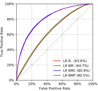
Figure 9: Impact of Finer-Grained Features (Variety) on ROC AUC for Predicting PU.
complication and we assess the quality of models. We now examine and evaluate the predictions for the different complications that we consider. We performed extensive tests using cross-validation methodology (see § 2.2.4), and we report on accuracy obtained from randomly chosen training and (disjoint) testing sets. Figure 13a shows a ROC curve obtained when predicting hospital death. We obtain a ROC AUC greater than 76%.
ROC curves and AUC obtained when predicting occurrence of pressure ulcers are shown on Figure 13b. Figure 13c shows the results for ICU admissions, and Figure 13d the results for hospital-acquired infections.
Overall, the system exhibits best accuracy for predicting the occurrence of hospital-acquired infections, pressure ulcers, and hospital deaths. Table 2 fur-ther illustrates detailed metrics on randomly selected datasets, with a thresh-old t = 0.5.
3.5. Velocity
We report on how fast the models can be generated with respect to the considered dataset size.
Three subtasks are particularly computationally-intensive: (i) the data pre-processing including prefiltering, joining and feature extraction from data (as explained in § 2.1.1 and 2.2.2), (ii) the construction (learning) of models (see § 2.2.3), and (iii) the evaluation of the model over a test dataset. Notice that since we perform cross-validation, the two latter steps are often grouped and performed repeatedly. Afterwards, once a model has been computed, its ex-ecution (for computing predictions) is very efficient. A cluster of machines is
50000 100000 150000 200000 250000 300000 350000 400000 Test population (number of patients)
60 % 65 % 70 % 75 % 80 %
Area under ROC Curve
BMP BMC BM
(a) Increasing volume leads to better ROC AUC.
50000 100000 150000 200000 250000 300000 350000 400000 Test population (number of patients)
52 % 54 % 56 % 58 % 60 % 62 % 64 % 66 % Recall BMP BMC BM
(b) Increasing volume leads to better recall.
Figure 10: Impact of volume on predictive performance with train and test sets of varying size (but with constant 2:1 ratio). Prediction of HAI.
20 % 40 % 60 % 80 % 100 % Train dataset ratio
60 % 65 % 70 % 75 % 80 %
Area under ROC Curve
BMP BMC BM
(a) Increasing volume tends to yield better ROC AUC.
20 % 40 % 60 % 80 % 100 %
Test population (number of patients) 56 % 58 % 60 % 62 % 64 % 66 % Recall BMP BMC BM
(b) Increasing volume tends to yield better recall.
Figure 11: Impact of volume on predictive performance with train sets of varying sizes, and same test set. Prediction of HAI.
20 % 40 % 60 % 80 % 100 % Train dataset ratio
4 % 6 % 8 % 10 % 12 % 14 % 16 % 18 %
Area under PR Curve
BMP BMC BM
Figure 12: PR AUC (train subsets of varying sizes and same test subset), when predicting hospital-acquired infections. Notice that classes are heavily imbalanced: hospital-acquired infections occur for 3% of all admissions. Metrics are reported for imbalanced (real) test sets.
then no longer needed: the model can be saved and transmitted (e.g. in PMML standard format) to be executed on a single commodity machine.
A BM model is computed in approximately 3.5 seconds from a training dataset of 800K instances, validated in 8 seconds on a test dataset of 400K instances, and executed in a negligible amount of time (a few ms) on a single instance (to obtain a prediction).
A more sophisticated BMP model (with more then 3 000 features) is computed in 20 seconds from a training dataset of 800K instances, validated in 14 seconds on a test dataset of 400K, and executed in a negligible amount of time (a few ms) on a single instance.
A BMC model (with more than 10 000 features) is computed in 108 seconds and validated in 29 seconds on datasets of similar sizes, and also executed in a negligible amount of time on a single instance.
Figure 14 illustrates the elapsed computation times in terms of the dataset size, for the different kind of models (from the simplest BM ones to the more complex BMP and BMC ones.
For the aforementioned computations to be possible, an additional one-time preprocessing stage is necessary to load and filter data (15s for loading and fil-tering patient data, and 4 minutes for loading, filfil-tering and joining with billing data stored in CSV format). This preprocessing stage is done only once; af-terwards and we restart from intermediate data that we store in the Parquet
0% 20% 40% 60% 80% 100% False Positive Rate
0% 20% 40% 60% 80% 100%
True Positive Rate
LR BMC (77.9%) LR BMP (77.4%)
(a) Predicting Death (AUC ≥ 77%).
0% 20% 40% 60% 80% 100% False Positive Rate
0% 20% 40% 60% 80% 100%
True Positive Rate
LR BMC (80.9%) LR BMP (80.5%)
(b) Pressure Ulcers (AUC ≥ 80%).
0% 20% 40% 60% 80% 100% False Positive Rate
0% 20% 40% 60% 80% 100%
True Positive Rate
LR BMC (65.6%) LR BMP (65.3%)
(c) ICU Admissions (AUC ≥ 65%).
0% 20% 40% 60% 80% 100% False Positive Rate
0% 20% 40% 60% 80% 100%
True Positive Rate
LR BMC (80.0%) LR BMP (80.3%)
(d) HAI (AUC ≥ 80%).
Figure 13: Predicting Hospital Death, Pressure Ulcers, ICU Admissions and Hospital-Acquired Infections with BMC and BMP Features (randomly picked datasets).
Metric Death ICU PU HAI Metric Definition True Positive Rate 65.1% 58.1% 68.4% 65.7% TP/P
True Negative Rate 75.4% 64.1% 78.0% 80.5% TN/N False Positive Rate 24.6% 35.9% 22.0% 19.5% FP/N False Negative Rate 34.9% 41.9% 31.6% 34.3% FN/P Negative Predictive Value 98.5% 97.3% 98.9% 98.9% TN/(TN+FN) Positive Predictive Value 7.9% 6.5% 7.9% 8.1% TP/(TP+FP) False Discovery Rate 92.1% 93.5% 92.1% 91.9% FP/(TP+FP)
Accuracy 75.1% 63.9% 77.8% 80.2% (TP+TN)/(P+N) Error 24.9% 36.1% 22.2% 19.8% (FP+FN)/(P+N)
Table 2: Detailed LR prediction metricsa on random train and test subsets, with notations
adopted from Fawcett [20]: TP is the number of true positives, FP: false positives, TN: true negatives, FN: false negatives, P=TP+FN and N=FP+TN.
Notice that classes are heavily imbalanced since complications typically occur for around 3% of all admissions. The presented metrics are computed on imbalanced (real) test subsets.
aTrue Positive Rate is also known as Hit Rate, Recall, and Sensitivity; True Negative Rate
is also known as Specificity; False Positive Rate as Fall-out; False Negative Rate as Miss Rate; and Positive Predictive Value as Precision.
format (which can be loaded in less than 10s). All these performance figures are obtained with the cluster of 5 machines set up to use 48GB of RAM per executor and 128 cores.
3.6. Scalability
We report on the extent to which model construction benefits from the availability of greater computational resources in the cluster of machines.
We make the computational resources of our cluster vary and study running times depending on the amount of memory available per executor and the total number of cores in the cluster. Figure 15a shows the elapsed times spent for a 3-fold cross validation process of a BM model depending on the cluster resources used. Each single time shown on Figure 15a thus corresponds to the total running time spent for 3 iterations of the construction and evaluation of a BM model on three randomly chosen datasets. Times are reported depending on two varying cluster resources: the amount of RAM per executor and the total number of cores available in the cluster. Figure 15a shows elapsed times when constructing BM models and Figure 15a shows elapsed times when constructing the more complex BMC models. Figure 16 illustrates the time variability of a single step of the cross-validation process (including time spent in splitting, normalizing features, training the model on one dataset, and evaluating the model on one dataset).
Figures all illustrate similar variations of computation times. Computation times decrease with the number of cores. We observe a particularly sharp de-crease in computation time when increasing the number of cores from 2 to 24. This overall behavior is similar independently of the amount of RAM available in each executor. We also observe that the computations tend to be faster when
100000 200000 300000 400000 500000 600000 700000 800000 Train population (number of patients)
0 20 40 60 80 100 120 140 160
Time of training and testing for 1 split (s)
BMP BMC BM
Figure 14: Times spent for constructing and testing models depending on dataset sizes.
more memory available in each executor. Overall, results show that the con-struction of simple and complex models greatly benefits from the distribution and the availability of more computational resources (mainly the number of cores) in the cluster.
3.7. Explainability
We pay particular attention to the explanability of the models that we gen-erate. In other terms, we do not only focus on numerical predictive modeling accuracy but also concentrate on generating models that offer opportunities for further clinical interpretation and understanding. Model explainability helps in building clinical knowledge and may guide the search of further models.
We thus further study the weights of the LR models that we generate. The weights of an LR model represent a summarization of the respective importance of features over the training dataset. As such, it is thus interesting to study how stable is this summarization with respect to different training datasets.
We constructed BMP models to predict hospital-acquired infections for 108 randomly selected train sets, and analysed the weights of all models. Specifically, we concentrate on the top 10 most important positive weights. In other terms, we retain the set S of all features f that such that f occurs in the top 10 most important positive weights in at least one of the 108 models. Only 12 drugs occur in S. These drugs are shown on Table 3a which presents the corresponding features sorted by their number of occurrences, and their identifier (not by weight which would require aggregation of some sort). We performed a similar analysis for the top 10 most important negative weights. Only 14 drugs form the most important negative weights, as shown in Table 3b.
0 20 40 60 80 100 120 140 Number of CPU Cores
100 200 300 400 500 600 Computation time (s) 8 GB 16 GB 32 GB 48 GB
(a) Construction of BM models.
0 20 40 60 80 100 120 140
Number of CPU Cores 200 400 600 800 1000 1200 1400 Computation time (s) 8 GB 16 GB 32 GB 48 GB (b) Construction of BMP models.
0 20 40 60 80 100 120 140 Number of CPU Cores
50 100 150 200 Computation time (s) min mean max
Figure 16: Times spent for a single step of the cross-validation process.
We also constructed BMC models for 102 randomly selected train sets. We analysed the weights of all models. This time, since these models use many more features, we pay attention to the topmost 20 positive and negative weights. Results are shown in Table 4 and 5, respectively.
We make the following observations:
• only the features indicated in the aforementioned tables form the most important weights of all models (there is no feature left with respect to the definition above);
• the majority of features retained this way appear in the most important weights of all models;
• the same obervations hold for the BMP and for the BMC models.
This illustrates the stability of weights and the robustness of the generated models with respect to the randomly selected train sets, opening the way for further clinical interpretation (beyond the scope of this article).
4. Related Works
A general overview of recent developments in big data in the context of biomedical and health informatics can be found in P´erez et al. [24]. With the broad adoption of EHRs systems, the development of techniques for improving the quality of clinical care has received considerable interest recently, especially from the AI community [25, 26, 27, 28, 29].
Most Important Positive Features Count 25025001018 CEFAZOLIN 108 25025002863 GENTAMICIN 108 25025004905 OXYCOD/ASA 108 25025005262 PIPERACILLIN/TAZO 108 25025006583 VANCOMYCIN 108 25025700053 ACETAMINOPHEN 108 25025800083 DEXTROSE SOLUTION 108 25025001030 CEFEPIME 90 25025800016 NACL 83 25025003050 HEPARIN NA FLUSH 72 25025000337 AMPICILLIN/SULBAC 43 25025003226 HYDROMORPHONE 36
(a) Positive Features
Most Important Negative Features Count 25025000520 AZITHROMYCIN 108 25025002815 FUROSEMIDE 108 25025003499 IPRATROPIUM 108 25025004224 METHYLPRED NA 108 25025004756 NITROGLYCERIN 108 25025004929 OXYTOCIN 108 25025700431 ASPIRIN 108 25025706196 VIT B1(THIAMINE) 108 25025000135 ALBUTEROL 106 25025001926 DINOPROSTONE 60 25025001966 DIPHTHERIA/TETANUS 33 25025704695 NICOTINE 14 25025003675 LEVALBUTEROL 2 25025003884 LORAZEPAM 1 (b) Negative Features
Table 3: The most important features in BMP models and the number of times they occur in the top 10 list of the most important weights, out of 108 randomly selected train sets.
Most Important Positive Features Count 250250065940000 VANCOMYCIN VL 500MG 102 250250065800000 VANCOMYCIN VL 500MG 102 250258001390000 DEXTROSE SOLUTION 100ML 102 250258000220000 NACL SOLUTION 100ML 102 250257000530000 ACETAMIN TAB 325MG (EA) 102 250250065950000 VANCOMYCIN VL 500MG 102 250250008220000 CA ACET TAB 667MG 102 250250065840000 VANCOMYCIN VL 500MG 102 mrci 102 250250052870000 PIPERACILLIN/TAZO VL 2/0.25GM 102 250250052630000 PIPERACILLIN/TAZO VL 2/0.25GM 102 250250049010000 OXYCOD/ASA TAB 4.5MG/325MG 102 250250028630000 GENTAMICIN VL 40MG/ML 2ML 102 250250010180000 CEFAZOLIN VL 1GM 102 250250010130000 CEFAZOLIN VL 1GM 102 adm type 2 101 250250003370000 AMP/SULBAC VL 3GM 94 250250100930000 SEVELAMER, RENAGEL CAP 403MG 87 250258000190000 NACL SOLUTION 100ML 78 250258001450000 DEXTROSE SOLUTION 100ML 69 250258000270000 NACL SOLUTION 100ML 50 250250010300000 CEFEPIME VL 1GM 20 250257000510000 ACETAMIN SUPP 325MG 11
Table 4: The most important positive features in BMC models and the number of times they occur in the top 10 list of the most important positive weights, out of 102 randomly selected train sets.
Most Important Negative Features Count 250250001200000 ALBUTEROL INH SOL 0.5% 1ML (5MG) 102 250250028190000 FUROSEMIDE VL 40MG 4ML 102 250257004340000 ASPIRIN TAB 325MG (EA) 102 250250105290000 OXYTOCIN VL 10U/ML 1ML 102 250250049270000 OXYTOCIN VL 10U/ML 1ML 102 250250047520000 NITROGLYCERIN OINT 2% 1GM 102 250250042270000 METHYLPRED NA VL 125MG 102 250250035010000 IPRATROPIUM INH SOL 0.02% 2.5ML 102 250250042240000 METHYLPRED NA VL 125MG 102 250250005200000 AZITHROMYCIN TAB 250MG 102 250250005110000 AZITHROMYCIN VL 500MG 102 250250019660000 DIPHTHERIA/TETANUS ADLT INJ 0.5ML 102 250250019260000 DINOPROSTONE VAG SUPP 10MG 102 250257004310000 ASPIRIN TAB 325MG (EA) 101 250257046890000 NICOTINE PATCH 21MG/DAY 99 250250036760000 LEVALBUTEROL, XOPENEX INH SOL 0.63MG/3ML 3ML 93 250250029250000 GUAIFEN SYRP 100MG/5ML 5ML 64 250250100600000 IPRATROPIUM/ALBUTEROL INH SOL 3ML 64 250250049290000 OXYTOCIN VL 10U/ML 1ML 63 250250052970000 PANTOPRAZOLE, PROTONIX I.V. VL 40MG 57 250257061960000 VIT B1(THIAMINE) TAB 100MG 53
age 50
250250001210000 ALBUTEROL INH SOL 0.5% 1ML (5MG) 34 250250043570000 MISOPROSTOL TAB 200MCG 14 250250028170000 FUROSEMIDE VL 40MG 4ML 13 250250028180000 FUROSEMIDE VL 40MG 4ML 5 250250021370000 ENOXAPARIN INJ 30MG 0.3ML 4
Table 5: The most important negative features in BMC models and the number of times they occur in the top 10 list of the most important negative weights, out of 102 randomly selected train sets.
The work of Luo et al. [28] adresses ICU mortality risk prediction with unsupervised feature learning techniques from timeseries of physiologic mea-surements (whereas we consider supervised techniques on prescribed drug data at admission). Lee et al. [25] introduce a method for the purpose of extracting phenotype information from EHRs and for providing analyses on phenotypes. Kuang et al. [26] propose a baseline regularization model for the task of finding new indications for existing drugs leveraging heterogeneous drug-related data based on EHRs. Li et al. [27] explore joint models for extracting mentions of drugs and their side effects, such as diseases that they cause. Zhang et al. [29] explore survival prediction with a focus on intermittently varying data.
Closely related works in terms of research objectives are the independent works performed simultaneously found in Avati et al. [30], Rajkomar et al. [31]. Authors develop a model for predicting all-cause mortality of patients from EHR data. The research objectives pursued are similar, and the methodology and the data used exhibit some similarities but with several important differences. First, [30] and [31] require “longitudinal” data in the sense that for making a prediction, their systems require historical data for the patient: it relies on historical observation windows and several observation slices: [30] uses 4 obser-vation slices and [31] uses data from 24 hours before hospital admission (and also after admission). Both systems require the knowledge of the patient situa-tion at several moments in time. In sharp contrast, our predictive system only
requires the list of drugs prescribed on the very first day of arrival at the hospital for making a prediction. Our prediction system is thus much more flexible and general, since it can be used with patients admitted for the first time with no known history. Second, [30] and [31] use deep neural network models whereas the current article presents results obtained with more classical models that: (i) perform faster on CPU machines, and (ii) are more intelligible: they offer more insights into the factors that influence the predictions, as emphasized in [32]. For instance, the weights computed by our models are stable and intelligible, allowing further interpretation (and fix if needed) by clinicians. Last but not least, to be able to operate without the need for historical data of patients, our models were trained with much more “transversal” data. [30] studies a popula-tion of 221 284 patients (216 221 hospitalizapopula-tions were studied in [31]), whereas our models are built from the automated analysis of more than 1.2 million of patients.
In fact, our work fundamentally differs from all these previous works by the initial assumed postulate from which we start. We formulate the hypothesis that the information required for identifying at-risk profiles is available in the initial patients’ drug prescription data at the time of hospital admission. In other terms, our system exclusively relies on analysing prescribed drug data of the day of admission. Previous studies that seeked to exploit EHR information with a similar postulate have mainly been developing score-based techniques. For instance the works found in [33, 34, 35, 5] also assume that the complexity of the patient’s medication regimen is a good indicator of the complexity of the patient’s condition. The existence of correlations between MRCI at admission and occurence of complications is empirically demonstrated in the work of Le-pelley et al. [5]. Compared to these works, we go further by (1) exploring how this information can be leveraged for predictive purposes (on large datasets) and (2) by considering finer-grained features, thanks to the distributed architecture, which allows to improve prediction accuracy. A simple score such as MRCI constitutes a rough approximation. For example, the same MRCI value may denote different situations with radically different evolution perspectives. Our fine-grained approach is more adapted to capture these differences. We showed that this leads to increased prediction accuracy.
Last but not least, we provide experimental evidence to validate our claim that big data perspectives such as volume and variety effectively help in extract-ing relevant information useful in a novel and concrete healthcare application for predicting complications.
5. Conclusion
We propose a novel method for identifying patients at risk of complications during their hospital stay, which is based exclusively on drug prescription data of the day of admission, for the purpose of developing adapted prevention. We illustrate how the volume and variety perspectives of big medical data improve the automatic identification of at-risk patients. Experimental results suggest that such systems might be especially useful for detecting patient profiles at
risk of hospital-acquired infections, pressure ulcers and death. This opens the door to promising research on the construction of further models. An advantage of our initial prototype system that of being adapted for deployment in hospi-tals as it is implementable in-house with modest hardware. It does not require neither external storage of sensitive medical data (thus avoiding additional is-sues of confidential data leakage), nor very expensive hardware (thanks to the distribution of data and computations).
References
[1] D. Levinson, Adverse Events in Hospitals: National Incidence among Medi-care Beneficiaries, Tech. Rep., Department of Health and Human Services, USA, https://oig.hhs.gov/oei/reports/OEI-06-09-00090.pdf, 2010. [2] C. Schaeffer, A. Haque, L. Booton, J. Halleck, A. Coustasse, Big Data Management in United States Hospitals: Benefits and Barriers., in: Pro-ceedings of the Business and Health Administration Association Annual Conference, J. Sanchez (Ed.), 129–138, 2016.
[3] R. Hillestad, J. Bigelow, A. Bower, F. Girosi, R. Meili, R. Scov-ille, R. Taylor, Can Electronic Medical Record Systems Trans-form Health Care? Potential Health Benefits, Savings, And Costs, Health Affairs 24 (5) (2005) 1103–1117, doi:10.1377/hlthaff.24.5.1103, https://www.healthaffairs.org/doi/pdf/10.1377/hlthaff.24.5.1103. [4] Frost, Sullivan, Drowning in Big Data? Reducing Information Technology
Complexities and Costs For Healthcare Organizations, Tech. Rep., Frost & Sullivan Company White Paper, 2012.
[5] M. Lepelley, C. Genty, A. Lecoanet, B. Allenet, P. Bedouch, M.-R. Mallaret, P. Gillois, J.-L. Bosson, Electronic Medication Regimen Complexity Index at admission and complications during hospitaliza-tion in medical wards: a tool to improve quality of care?, Interna-tional Journal for Quality in Health Care doi:10.1093/intqhc/mzx168, URL http://dx.doi.org/10.1093/intqhc/mzx168.
[6] H. Quan, V. Sundararajan, P. Halfon, A. Fong, B. Burnand, J.-C. Luthi, L. D. Saunders, C. Beck, T. Feasby, W. Ghali, Coding algorithms for defining comorbidities in ICD-9-CM and ICD-10 administrative data., Med Care 43 (11) (2005) 1130–1139, https://www.ncbi.nlm.nih.gov/pubmed/16224307.
[7] D. Roosan, M. Samore, M. Jones, Y. Livnat, J. Clutter, Big-Data Based Decision-Support Systems to Improve Clinicians’ Cognition, in: Proceed-ings - 2016 IEEE International Conference on Healthcare Informatics, ICHI 2016, Institute of Electrical and Electronics Engineers Inc., 285–288, doi: 10.1109/ICHI.2016.39, 2016.
[8] M. Armbrust, R. S. Xin, C. L., Y. H., D. L., J. K. Bradley, X. Meng, T. Kaf-tan, M. Franklin, A. Ghodsi, M. Zaharia, Spark SQL: Relational Data Pro-cessing in Spark, in: SIGMOD, 1383–1394, doi:10.1145/2723372.2742797, http://doi.acm.org/10.1145/2723372.2742797, 2015.
[9] Z. Czech, G. Havas, B. Majewski, Perfect Hashing, Theor. Com-put. Sci. 182 (1-2) (1997) 1–143, doi:10.1016/S0304-3975(96)00146-6, http://dx.doi.org/10.1016/S0304-3975(96)00146-6.
[10] M. Zaharia, R. S. Xin, P. Wendell, T. Das, M. Armbrust, A. Dave, X. Meng, J. Rosen, S. Venkataraman, M. Franklin, A. Ghodsi, J. Gon-zalez, S. Shenker, I. Stoica, Apache Spark: a unified engine for big data processing, Commun. ACM 59 (11) (2016) 56–65, doi:10.1145/2934664, URL http://doi.acm.org/10.1145/2934664.
[11] X. Meng, J. Bradley, B. Yavuz, E. Sparks, S. Venkataraman, D. Liu, J. Free-man, D. Tsai, M. Amde, S. Owen, D. Xin, R. Xin, M. Franklin, R. Zadeh, M. Zaharia, A. Talwalkar, MLlib: Machine Learning in Apache Spark, CoRR abs/1505.06807, http://arxiv.org/abs/1505.06807.
[12] D. Cox, The Regression Analysis of Binary Sequences, Journal of the Royal Statistical Society. Series B (Methodological) 20 (2) (1958) 215–242, ISSN 00359246, http://www.jstor.org/stable/2983890.
[13] J. Suykens, J. Vandewalle, Least Squares Support Vector Machine Classifiers, Neural Processing Letters 9 (3) (1999) 293–300, ISSN 1573-773X, doi:10.1023/A:1018628609742, URL http://dx.doi.org/10.1023/A:1018628609742.
[14] J. Quinlan, Induction of decision trees, Machine learning 1 (1) (1986) 81–106.
[15] J. Han, J. Pei, Y. Yin, R. Mao, Mining Frequent Patterns without Can-didate Generation: A Frequent-Pattern Tree Approach, Data Min. Knowl. Discov. 8 (1) (2004) 53–87, doi:10.1023/B:DAMI.0000005258.31418.83, http://dx.doi.org/10.1023/B:DAMI.0000005258.31418.83.
[16] L. Maaten, G. Hinton, Visualizing data using t-SNE, Journal of Machine Learning Research 9 (Nov) (2008) 2579–2605.
[17] D. Merkel, Docker: Lightweight Linux Containers for Consistent De-velopment and Deployment, Linux J. 2014 (239), ISSN 1075-3583, http://dl.acm.org/citation.cfm?id=2600239.2600241.
[18] J. George, Y. Phun, M. J. Bailey, D. C. Kong, K. Stewart, Develop-ment and Validation of the Medication Regimen Complexity Index, An-nals of Pharmacotherapy 38 (9) (2004) 1369–1376, doi:10.1345/aph.1D479, http://dx.doi.org/10.1345/aph.1D479.
[19] A. Paquin, K. Zimmerman, T. Kostas, L. Pelletier, A. Hwang, M. Simone, L. Skarf, J. Rudolph, Complexity perplexity: a systematic review to de-scribe the measurement of medication regimen complexity, Expert Opinion on Drug Safety 12 (6) (2013) 829–840, doi:10.1517/14740338.2013.823944. [20] T. Fawcett, An Introduction to ROC Analysis, Pattern Recogn. Lett. 27 (8) (2006) 861–874, doi:10.1016/j.patrec.2005.10.010, http://dx.doi.org/10.1016/j.patrec.2005.10.010.
[21] D. Powers, Evaluation: From precision, recall and f-measure to roc., in-formedness, markedness & correlation, Journal of Machine Learning Tech-nologies 2 (1) (2011) 37–63.
[22] I. Guyon, V. Lemaire, M. Boull´e, G. Dror, D. Vogel, Analysis of the KDD Cup 2009: Fast Scoring on a Large Orange Customer Database, in: Proc. of KDD-Cup competition, vol. 7 of JMLR Proceedings, 1–22, http://www.jmlr.org/proceedings/papers/v7/guyon09.html, 2009. [23] J. Davis, M. Goadrich, The relationship between Precision-Recall
and ROC curves, in: ICML, 233–240, doi:10.1145/1143844.1143874, http://doi.acm.org/10.1145/1143844.1143874, 2006.
[24] J. A. P´erez, C. C. Y. Poon, R. D. Merrifield, S. T. C. Wong, G. Yang, Big Data for Health, IEEE J. Biomedical and Health Informatics 19 (4) (2015) 1193–1208, doi:10.1109/JBHI.2015.2450362, https://doi.org/10.1109/JBHI.2015.2450362.
[25] W. Lee, Y. Lee, H. Kim, I. Moon, Bayesian Nonparamet-ric Collaborative Topic Poisson Factorization for Electronic Health Records-Based Phenotyping, in: IJCAI, 2544–2552, http://www.ijcai.org/Proceedings/16/Papers/362.pdf, 2016.
[26] Z. Kuang, J. A. Thomson, M. Caldwell, P. L. Peissig, R. M. Stew-art, D. Page, Baseline Regularization for Computational Drug Reposi-tioning with Longitudinal Observational Data, in: IJCAI, 2521–2528, http://www.ijcai.org/Proceedings/16/Papers/359.pdf, 2016.
[27] F. Li, Y. Zhang, M. Zhang, D. Ji, Joint Models for Extracting Ad-verse Drug Events from Biomedical Text, in: IJCAI 2016, 2838–2844, http://www.ijcai.org/Proceedings/16/Papers/403.pdf, 2016.
[28] Y. Luo, Y. Xin, R. Joshi, L. Celi, P. Szolovits, Predicting ICU Mortality Risk by Grouping Temporal Trends from a Multi-variate Panel of Physiologic Measurements, in: AAAI, 42–50,
https://www.aaai.org/ocs/index.php/AAAI/AAAI16/paper/view/11843/11562.pdf, 2016.
[29] J. Zhang, L. Chen, A. Vanasse, J. Courteau, S. Wang, Sur-vival Prediction by an Integrated Learning Criterion on In-termittently Varying Healthcare Data, in: AAAI, 72–78,
http://aaai.org/ocs/index.php/AAAI/AAAI16/paper/view/11873/11566.pdf, 2016.
[30] A. Avati, K. Jung, S. Harman, L. Downing, A. Y. Ng, N. H. Shah, Im-proving Palliative Care with Deep Learning, in: Proceedings of the IEEE International Conference on Bioinformatics and Biomedicine, 311–316, https://arxiv.org/pdf/1711.06402.pdf, 2017.
[31] A. Rajkomar, E. Oren, K. Chen, A. M. Dai, N. Hajaj, P. J. Liu, X. Liu, M. Sun, P. Sundberg, H. Yee, K. Zhang, G. E. Duggan, G. Flores, M. Hardt, J. Irvine, Q. Le, K. Litsch, J. Marcus, A. Mossin, J. Tansuwan, D. Wang, J. Wexler, J. Wilson, D. Ludwig, S. L. Volchenboum, K. Chou, M. Pearson, S. Madabushi, N. H. Shah, A. J. Butte, M. Howell, C. Cui, G. Corrado, J. Dean, Scalable and accurate deep learning for electronic health records, Tech. Rep., eprint arXiv:1801.07860: https://arxiv.org/abs/1801.07860, 2018.
[32] R. Caruana, Y. Lou, J. Gehrke, P. Koch, M. Sturm, N. Elhadad, Intelligible Models for HealthCare: Predicting Pneumonia Risk and Hospital 30-day Readmission, in: Proceedings of the 21th ACM SIGKDD International Conference on Knowledge Discovery and Data Mining, Sydney, NSW, Australia, August 10-13, 2015, 1721–1730, doi:10.1145/2783258.2788613, http://doi.acm.org/10.1145/2783258.2788613, 2015.
[33] H. Schoonover, C. Corbett, D. Weeks, M. Willson, S. Setter., Pre-dicting potential postdischarge adverse drug events and 30-day un-planned hospital readmissions from medication regimen complexity., J Patient Saf. 10 (4) (2014) 186–91, doi:10.1097/PTS.0000000000000067, https://www.ncbi.nlm.nih.gov/pubmed/25408236.
[34] M. Willson, CL.Greer, D. Weeks., Medication regimen complex-ity and hospital readmission for an adverse drug event., Ann Pharmacother. 48 (1) (2014) 26–32, doi:10.1177/1060028013510898., https://www.ncbi.nlm.nih.gov/pubmed/24259639.
[35] F. Yam, T. Lew, S. Eraly, H. Lin, J. Hirsch, M. Devor, Changes in medica-tion regimen complexity and the risk for 90-day hospital readmission and/or emergency department visits in U.S. Veterans with heart failure., Res So-cial Adm Pharm. 12 (5) (2016) 713–21, doi:10.1016/j.sapharm.2015.10.004., https://www.ncbi.nlm.nih.gov/pubmed/26621388.