Control using neural networks and adaptive control for cooling rate in GMA welding

Control Using Neural Networks and Adaptive Control for

Cooling Rate in GMA Welding

by

Isamu Okamura

Kogaku-shi (B.E.), University of Tokyo (1982) Submitted to the Department of

Mechanical Engineering in Partial Fulfillment of the Requirements for the Degree of

Master of Science

at the

Massachusetts Institute of Technology

© 1994 Isamu Okamura All rights reserved

The author hereby grants to MIT permission to reproduce and to distribute publicly paper and electronic copies of this thesis

document in whole or in part.

I)j

t

Signature of Author... ... ...

wepartment of Mechanical Engineering May 6, 1994

Certified by ... ...

David E. Hardt Professor, Department of Mechanical Engineering Thesis Supervisor

Accepted

by ...

:...

...

Ain A. Sonin Chairman, Departmental Committee on Graduate Studies

Control Using Neural Networks and Adaptive Control for

Cooling Rate in GMA Welding

by

Isamu Okamura

Submitted to the Department of Mechanical Engineering on May, 1994 in partial fulfillment of the requirements for the Degree of Master of Science in Mechanical Engineering

Abstract

The dynamic behavior of cooling rate during gas metal arc welding (GMAW) has been studied experimentally using an infrared pyrometer which scans the weldment using an oscillating mirror. The purpose of this study is to learn how the input variables of wire feed rate and travel speed affect the cooling rate. The experiments show that the wire feed rate has little effect on the steady-state cooling rate, although a distinct change of the temperature distribution is observed. By contrast, the travel speed has a strong effect on the cooling rate.

A comparison between analytical models and the actual measurement is made. The analytical models are based on Green's function for the partial differential equations of the heat transfer. They do not succeed in explaining the small effect of the wire feed rate on the cooling rate. On the other hand, there is good correspondence between the analytical model and the actual measurement for the dynamic behavior of the cooling rate. The analytical model, together with the experiment results, suggests the cooling rate should be controlled by the travel speed. The control should also accommodate the nonlinearity and the varying time-delay that are observed.

Two types of control schemes, linear adaptive control and nonlinear control using neural networks are proposed to achieve high performance. The adaptive control adjusts the parameters of its linear model to the perturbation caused by the nonlinearity. The control using neural networks regulates the cooling rate by directly employing a nonlinear model. Thus, both schemes can accommodate the nonlinear nature of the process.

A one-step-ahead adaptive control method is used as the adaptive controller. Some practical considerations, such as a weighing factor, an integrator and a constrained parameter estimation are discussed. Two types of model structures are proposed to cope with the varying time-delay. A recursive least-square algorithm is used as the on-line estimator. The estimation by this algorithm is fast enough to accommodate the nonlinearity of the process. For the controller using neural networks, first the characteristics of neural networks are investigated. The investigation suggests control based on Smith's principle because of the process delays. The design methods, such as the parallel identification based on a conjugate gradient algorithm and the controller design based on a back-propagation method with a distal system, are proposed. Some limitations that come from the complexity of neural computation and nonlinear identification are found.

The performances of both control schemes are shown by simulation using the analytical model. Both control schemes bring about quite satisfactory results, showing better performance than PI control.

Thesis Supervisor: Dr. David E. Hardt

Acknowledgments

I wish to express my deepest gratitude to Professor David E. Hardt, my thesis advisor, for giving me the opportunity to work on this project and learn from his expertise in process control. His guidance and suggestions were invaluable throughout my research. I also thank professor Hardt for his patience and time in reading this thesis.

I would like to thank other members of the faculty at MIT for giving me a chance to understand and learn theories associated with control. In particular, I would like to thank Professor Haruhiko Asada for his teaching and advise on the control using neural networks.

I also wish to thank Professor Toshiyuki Kitamori and Professor Shuji Yoshizawa at the University of Tokyo for their encouragement and advice for my study at MIT.

I would like to express my appreciation to my colleagues in our laboratory, Andrew Parris, Benny Budiman, Christopher Ratliff, Dan Walczyk, Robert Bakkestuen, and Upi Ummethala for their friendship and technical advice.

My special appreciation goes to my friends, Mr. David Mazzola, and Dr. Jang Boem Seong who offered me invaluable support of my life in the United States. Their heartwarming hospitality and encouragement kept me going through my career at MIT.

I am very thankful to my parents for their love, support, and encouragement through out my life. I would like to express my gratitude to my wife, Keiko and my children, Shun and Reina. Their assistance and love always have cheered me up, and led me to the goal of completion. I would like to dedicate this thesis to them.

Finally, I would like to gratefully acknowledge Kawasaki Steel Corporation for giving me the opportunity to study at MIT. Special thanks go to Mr. Kazushi Baba, and Mr. Tadaaki Iwamura for their encouragement and support.

This project was supported by the U.S. Department of Energy under contract number DE-FG02-85ER1333 1.

Table of contents

Table of contents ...

4

List of Figures ... 7

List of Tables ...

9

Chapter 1 Introduction ...

10

1.1 Organization of the thesis ... 13

Chapter 2 Measurement of Cooling Rate during GMAW ... 14

2.1 Measurement system ... 14

2.1.1 Specifications of measurement system ... 14

2.1.2 Conversion of intensity of radiation to temperature ... 16

2.1.3 Fitting by spline function ... 17

2.1.4 Other issues for measurement system ... 21

2.2 Measurement ... ... 22

2.2.1 Measured variables ... 22

2.2.2 Measurement conditions ... 25

2.2.3 Result of measurement ... 26

2.3 Remarks ... 34

Chapter 3 Dynamic Model of Temperature Distribution ... 39

3.1 Analytical models ... 40

3.2 Choice of model ... ... 48

3.2.1 Effect of thickness ... ... 48

3.2.2 Effect of width ... ... 48

3.2.3 Effect of Gaussian distributed heat input ... 49

3.2.4 Effect of heat transfer coefficient ... 50

3.2.5 Choice of model ... 51

3.3 Dynamic behavior of temperature distribution ... 52

3.3.1 Parameters of model ... ... 52

3.3.2 Simulation ... 53

3.3.3 Dynamic behavior for step-wise change of inputs ... 55

3.4 Remarks ... 58

Chapter 4 Problems in Control of Cooling Rate ... 60

4.1 Nonlinearity and time-delay ... 60

4.2 Results of PI control ... 62

4.2.1 PI controller design ... ... 62

4.3 Conclusions ... ... 66

Chapter 5 Control for Nonlinear and Time-Delay Systems ... 67

5.1 General review of control system design ... 67

5.1.1 Models ... ... 68

5.1.2 Objectives of control ... 69

5.1.3 Stability and Performance ... 69

5.1.4 Control scheme ... 70

5.1.5 What shall we discuss in this chapter? ... 72

5.2 Models for discrete-time systems ... 73

5.2.1 Advantages and disadvantages of linear models and nonlinear models ... 73

5.2.2 Linear models ... 74

5.2.3 Nonlinear models ... 75

5.3 Neural networks ... ... 77

5.3.1 Multilayer neural networks and back-propagation ... 77

5.3.2 Recurrent networks and identification ... 79

5.3.3 Radial basis networks ... 81

5.4 Identification for linear systems and nonlinear systems ... 83

5.4.1 Linear system identification ... 83

5.4.2 Nonlinear system identification ... 87

5.4.3 Some comments on nonlinear identification ... 93

5.5 Control dealing with time-delay ... 96

5.5.1 Smith's principle ... 96

5.5.2 Other methods for time-delay ... 98

5.6 Feed-back control for nonlinear systems ... 99

5.6.1 Feed-back linearization ... 99

5.6.2 One-step-ahead predictive control ... 103

5.6.3 Modification of nonlinear one-step-ahead predictive control ... 111

5.6.4 Other nonlinear control with fixed parameters ... 113

5.7 Adaptive control ... ... 114

5.7.1 Linear adaptive control ... 116

5.7.2 Nonlinear adaptive control ... 119

5.8 Control for cooling rate ... ... 121

Chapter 6 Application of linear adaptive control to cooling rate ... 123

6.1 Choice of adaptive controller ... 123

6.2 Practical aspect of control design ... 127

6.2.1 Modifications of least square algorithm ... 127

6.2.2 Constrained parameter estimation ... 128

6.2.3 Weighted one-step-ahead control with an integrator ... 129

6.2.4 Scaling variables ... ... ... 130

6.2.5 Modified one-step-ahead adaptive controller ... 131

6.3.1 Type 1: Approximation of time-delay ... 133

6.3.2 Type 2: Multi-model structure ... 134

6.4 Performance of estimation and control ... 136

6.4.1 Performance of Type 1 model structure ... 136

6.4.2 Performance of Type 2 model structure ... 146

6.5 Concluding remarks ... 153

Chapter 7 Application of Control Using Neural Networks

to Cooling Rate ...

155

7.1 Back-propagation method ... 156

7.1.1 Algorithm of back-propagation ... 156

7.1.2 Back-propagation with a distal system ... 157

7.2 Identification by neural networks ... ... 160

7.2.1 Series-parallel identification and parallel identification ... 160

7.2.2 Series-parallel estimation and parallel estimation ... ... 161

7.2.3 Conjugate gradient method for parallel identification ... 163

7.3 Approximation and identification by neural networks ... 165

7.3.1 Approximation of nonlinear systems ... ... 165

7.3.2 Parameter identification of dynamic systems ... 168

7.3.3 Concluding remarks ... 175

7.4 Selection of control using neural networks ... 176

7.4.1 Feed-back control with fixed parameters or adaptive control?.. 176

7.4.2 Model structure ... 177

7.4.3 Order of model ... 177

7.4.4 Treatment of time-delay ... ... 178

7.4.5 Control based on Smith's principle ... 179

7.5 Identification by neural networks for cooling rate ... 181

7.5.1 input given for the identification ... 181

7.5.2 Result of series-parallel identification ... 182

7.5.3 Result of parallel identification ... 183

7.6 Control using neural networks for cooling rate ... 186

7.6.1 Selection of control law for inner loop ... 186

7.6.2 Back-propagation with a distal system ... 187

7.6.3 Performance of inner loop control ... 190

7.6.4 Outer loop control ... 192

7.6.5 Comparison with other methods ... 195

7.7 Concluding remarks ... 198

Chapter 8 Comparison between adaptive control and control using

Chapter 9 Conclusions ...

...

207

9.1 Future work ... ... 207

Appendix A ... 210

R eferences ... 220

List of figures

Fig. 2.1.1 Layout of measurement system . ... 15

Fig. 2.1.2 Synchronization of sampling ... 15

Fig. 2.1.3 Comparison between measurements by pyrometer and thermocouple.17 Fig. 2.1.4 Example of temperature distribution ... 18

Fig. 2.1.5 Fitting by the 3rd order polynomial ... 19

Fig. 2.1.6 Fitting for transient-state temperature distribution ... 20

Fig. 2.1.7 Fitting by spline function ... 21

Fig. 2.2.1 Result of measurement for case A ... 27

Fig. 2.2.2 Result of measurement for case B ... 29

Fig. 2.2.3 Result of measurement for case C ... 31

Fig. 2.2.4 Result of measurement for case D ... 33

Fig. 2.2.5 Typical pattern of measured variables ... 34

Fig. 2.2.6 Change in temperature distribution by wire feed rate ... 35

Fig. 2.2.7 Steady-state temperature distribution (Travel speed 4 mm/sec) ... 37

Fig. 2.2.8 Change in temperature distribution by travel speed ... 38

Fig. 3.2.1 Effect of thickness ... 49

Fig. 3.2.2 Effect of width ... 49

Fig. 3.2.3 Effect of Gaussian heat source ... 50

Fig. 3.2.4 The effect of heat transfer coefficient ... 51

Fig. 3.3.1 Shape of O(w', ) data ... ... 54

Fig. 3.3.2 Shift of O(w', r) data ... 54

Fig. 3.3.3 Response by step-wise change of wire feed rate ... 55

Fig. 3.3.4 Response by step-wise change of travel speed ... 57

Fig. 3.3.5 Change of temperature distribution after the step-wise change of travel speed ... 57

Fig. 3.3.6 Change of temperature distribution after the step-wise change of wire feed rate ... 58

Fig. 4.1.1 Step response by travel speed ... .. 61

Fig. 4.2.1 Values for R and L in the response of cooling rate ... 62

Fig. 4.2.2 Step response of a first order system ... 62

Fig. 4.2.3 Response of PI control (Ziegler and Nichols method) ... 64

Fig. 4.2.4 Response of PI control ... 64

Fig. 5.1.1 Block diagram of control system ... 69

Fig. 5.1.2 Feasible control methods ... ... 72

Fig. 5.3.1 Feed-forward multilayer neural network ... 78

Fig. 5.3.2 Back-propagation ... ... 79

Fig. 5.3.3 Identification of nonlinear plants using neural network ... 81

Fig. 5.3.4 Radial basis networks ... 82

Fig. 5.4.1 Comparison between incremental gradient method and recursive least square method ... 94

Fig. 5.5.1 Smith's principle ... 97

Fig. 5.7.1 Block diagram of MRAC ... 114

Fig. 5.7.2 Block diagram of STR ... 115

Fig. 5.7.3 Nonlinear MRAC using neural network ... 120

Fig. 5.7.4 Nonlinear STR using neural network ... 121

Fig. 6.2.1 Constrained parameter estimation ... 128

Fig. 6.2.2 Adaptive control ... 132

Fig. 6.3.1 Step response ... 133

Fig. 6.4.1 The result of prediction for varied input magnitude ... 137

Fig. 6.4.2 The result of prediction for PRBS ... 138

Fig. 6.4.3 One-step-ahead control without integrator ( A =0.05) ... 140

Fig. 6.4.4 One-step-ahead control without integrator (A =0.03) ... 141

Fig. 6.4.5 One-step-ahead control without integrator ( A =0.01) ... 142

Fig. 6.4.6 Weighted one-step-ahead control with integrator (No limit on P/) .. 144

Fig. 6.4.7 Weighted one-step-ahead control with integrator (P0 >_{0) ... 145}

Fig. 6.4.8 Weighted one-step-ahead control with type 2 structure (A = 0.03, y = 0.7) ... 148

Fig. 6.4.9 Weighted one-step-ahead control with type 2 structure (A = 0.03, y - 0.8) ... 149

Fig. 6.4.10 Change of model structure ( = 0.03, y = 0.8) ... 150

Fig. 6.4.11 Comparison between one-step-ahead-control and PI control ... 151

Fig. 6.4.12 Change of model structure ... 152

Fig. 6.4.13 One-step-ahead-control and PI control ( = 0.1, y = 0.5) ... 153

Fig. 7.1.1 Neural network with a distal system ... 158

Fig. 7.3.1 Approximation by neural networks (Single input single output case). 166 Fig. 7.3.2 Approximation by neural networks (Two inputs single output case) . 167 Fig. 7.3.3 Response to pure sinusoidal input ... 170

Fig. 7.3.4 Response to step input with various magnitude ... 170

Fig. 7.3.5 Mapping created by neural network ... .. 171

Fig. 7.3.6 Response to step input with various magnitude ... 172

Fig. 7.3.7 Distribution of input-output pairs ... 173

Fig. 7.3.8 Response to sinusoidal input with various frequencies ... 173

Fig. 7.3.9 Mapping created by neural network ... 174

Fig. 7.5.2 Series-parallel identification ... ... 183

Fig. 7.5.3 Parallel identification ... 184

Fig. 7.5.4 Mapping y(t + 1) = NN(y(t),u(t)) ... 185

Fig. 7.6.1 Nonlinear controller u(t) = NNc(y(t),h) ... 188

Fig. 7.6.2 Response of the combined neural networks ... 189

Fig. 7.6.3 Block diagram of the inner loop control ... 190

Fig. 7.6.4 Predictive control ... 191

Fig. 7.6.5 Feed-back linearization (k=0.5) ... 191

Fig. 7.6.6 Block diagram of the control based on Smith's principle ... 192

Fig. 7.6.7 Feed-back control by Smith's principle ... 193

Fig. 7.6.8 Feed-back control by Smith's principle for a disturbance of 10 °c/sec. 194 Fig. 7.6.9 _{Block diagram of control by modified Smith's principle ... 195}

Fig. 7.6 10 Control by modified Smith's principle for disturbance 10[°c/sec] .... 196

Fig. 7.6.11 Comparison between control using neural networks and PI control . 197 Fig. 8.1.1 Disturbance rejection by three control methods ... 201

Fig. 8.1.2 Performance for plant perturbation (a) ... 202

Fig. 8.1.3 Performance for plant perturbation (b) ... 203

Fig. 8.1.4 Performance for plant perturbation (c) ... 204

Fig. 8.1.5 Performance for plant perturbation (d) ... 205

List of Tables

Chapter 1

Introduction

Joining is an important and necessary aspect of manufacturing operations. It is achieved by various methods. Among them the arc welding is thought of as the most fundamental method for joining metals. The arc welding process involves partial melting and fusion of the joint between two workpieces, which are achieved by the thermal energy established between an electrode and materials. Therefore, the modification of both the geometry and properties of materials always takes place during welding. Weld quality takes metallurgical and mechanical features such as loading capacity, fracture toughness, oxidation and corrosion resistance, and geometric tolerance of the joint. The final objective of the welding control is, therefore, to establish a control system to get satisfactory results for these weld quality factors.

This thesis deals with the control for gas metal arc welding (GMAW). The control should have a feed-back form based on an in-process measurement. However, the above-mentioned weld quality factors are quite hard to measure. Thus, an indirect approach for controlling the weld quality is used. The key outputs for GMAW, which are associated with the weld quality, are three geometry features (bead width, height, and depth), and two thermal features (heat affected zone width and centerline cooling rate). A multivariable scheme for the control of these features has been presented by Hardt (1990). The typical inputs of this control are the travel speed of the torch and the wire feed rate as shown in Fig. 1.1.1. It is quite important to know and understand how such inputs affect these outputs.

Our research is motivated by the desire to control the mass transfer rate (mass fed into the workpiece per a unit length) and the centerline cooling rate. A control structure using fuzzy control and neural networks has been presented by Einerson et al for this problem (1992). Since the dynamic behavior of the system has not been discussed in this paper, we have a fundamental question as to the decoupleness of the mass transfer and the cooling rate. The simplest model describing the temperature geometry in the workpiece, which was derived by Rosenthal (1946), is given by

ing gas electrode ozzle e guide and tact tube ielding gas tal Fig. 1.1.1 GMAW

where T denotes the temperature, Tois the ambient temperature, Q is the heat input, A is the thermal conductivity, and r is the distance from a torch. The equation (1.1.1) results in the model for the cooling rate:

CR = -2,rA(Tc - To)2 Q

(1.1.2)

where CR is the cooling rate at the critical temperature To, and v is the travel speed. The mass transfer is simply proportional to the ratio of the wire feed rate and the travel speed. Since almost all heat would be supplied by the molten electrode,

Mass transfer = f o Q

V V

f: Wire feed rate

is also true for pure arc process as well. Therefore, the mass transfer is closely coupled to the cooling rate via the term Q/v. From this point of view, Rosenthal's model shows that it is impossible to control the centerline cooling rate and the mass transfer at the same

(1.1.3)

time. However, as will be shown later, a new careful analysis and experimental data show that this is not the case.

Therefore, the first objective of this thesis is to depict the steady-state and dynamic behavior of the centerline cooling rate. Although extensive investigation has been done by Doumanidis and Hardt (1988, 1989) on the treatment of thermal features from a view-point of control scheme, little description for the detailed behavior of the centerline cooling rate has been discussed for these two inputs.

The other purpose of this thesis is to design the control system for the centerline cooling rate. As Doumanidis and Hardt (1988, 1989) pointed out, the control must deal with a nonlinearity in the dynamics of the cooling rate. In this thesis two types of controls, linear adaptive control and control using neural networks, are presented to deal with the nonlinearity.

The linear adaptive control is used as a system to adjust a linear model to the nonlinear dynamics of the process and to control it through the linear model. By 1980 considerable theoretical progress had been made in the scheme of adaptive control

(Narendra and Annaswamy (1989), Astr6m (1989), Goodwin and Sin (1984) and Landau (1981)). The applications of the adaptive control to the welding process have been presented by Suzuki (1988), Song (1992), and Doumanidis (1988). These investigations show satisfactory results for the control of the welding process. From practical point of view, the implementation of an adaptive control is rather simple. However, the control sometimes shows an undesirable behavior such as a saturation and an instability due to the violation of the strong assumptions of most adaptive schemes. Therefore an appropriate consideration should be given to the implementation of the algorithm. In this thesis we focus our interest on the practical implementation of the control for the cooling rate.

Recently, control using neural networks has been attracting the interest of many researchers. (White et al. (1992)) The expectation for neural networks is that they will give us a tool designing a nonlinear controller. Many control schemes using neural networks have been proposed. However the theoretical treatments are still under research. Little successful application of control using neural networks has been reported. Neural networks simply provide a model describing nonlinear systems, therefore various nonlinear control schemes are applicable. In this thesis first the possible configuration of the control using neural networks for the cooling rate is studied, considering the limitations of neural networks and the nature of the process of the cooling rate. Then, the design methods and the performance of this control are discussed.

1.1 Organization of the thesis

Chapter 2 describes the experiment for the cooling rate that was conducted to show the effect of the inputs of wire feed rate and travel speed. Chapter 3 presents an analytical model for analyzing the dynamics of the cooling rate. This model is used for designing the controller for the cooling rate. Chapter 4 discusses the nature of the cooling rate process based on the results in Chapter 2 and Chapter 3. In this chapter the performance of conventional PI controller is shown to demonstrate the problems of the control for the cooling rate. Chapter 5 reviews nonlinear controls to study the feasible nonlinear control methods for the cooling rate. Chapter 6 deals with adaptive control for the cooling rate. In this chapter practical implementation issues are discussed. Chapter 7 presents control using neural networks. In this chapter the drawbacks of the neural networks are first investigated. Then we discuss the implementation, considering the drawbacks and the nature of the cooling rate dynamics. Finally conclusions are made in Chapter 8.

Chapter 2

Measurement of Cooling Rate during GMAW

It is quite important to know and understand the nature of the process when we design the controller. This chapter presents the measurement of the center-line cooling rate during GMAW for this purpose. The objective of the measurement is to learn how the input variables of wire feed rate and travel speed affect the cooling rate.

2.1 Measurement system

Some measurement systems have been presented for measuring thermal geometry during welding. (Doumanidis and Hardt (1988, 1989), Lukens and Morris (1982), and Chin, Madsen and Goodling (1983)) All the systems use an infrared camera, which usually require cooling by liquid nitrogen, and is a rather expensive sensor.

However, the purpose of our experiment is simply to measure the temperatures along a line on the weldment surface. Therefore, a simpler configuration of measurement system is proposed. It is composed of an infrared pyrometer that is widely used in the industry and an oscillating mirror.

2.1.1 Specifications of measurement system

Figure 2.1.1 shows the measurement system, whose specification is shown in Table 2.1. About 45 output signals proportional to the radiation from the weld surface behind the torch are acquired by a PC acquisition board every scanning of the mirror. The sampling timing is synchronized with the oscillation of the mirror by a pulse signal that is given by the step motor. (Fig. 2.1.2) The signals from the pyrometer are converted to temperatures by the method discussed in Section 2.1.2. The temperature distributions on the weldment are acquired every 0.5 sec. The acquired temperatures are fit to a spline function composed of piece-wise third-order polynomials to eliminate noise caused by the arc. The centerline cooling rate is calculated based on the polynomials.

Fig. 2.1.1 Layout of measurement system Start pulse Direction f rotation

I

I Abot ut 45 data Abou About 45 datat 45 data

Sampling |

by PC Il l~l~

l...ll I l~

I lllll...ll

Fig. 2.1.2 Synchronization of sampling Table 2.1 Specification of measurement system Pyrometer

Type Accufiber model 100c (Accufiber Division

Luxtron Corp.)

Photocell _{Silicon cell}

Wave length of pyrometer 950 nm

Output Intensity proportional to radiation

Band width of output 10000 Hz

Oscillating mirror

Oscillation cycle of mirror 1 Hz: Temperature distribution is measured every 500 msec

Location of mirror Height: About 100 mm, Distance from arc: About 50 mm

Angle of oscillation 27 degree: Temperature distribution within about 100 mm from the arc is measured. Data acquisition

Data acquisition method Data acquisition board in PC

Data acquisition interval 10 msec: About 45 data are sampled per a scanning of mirror I I I I I I --- ----

-2.1.2 Conversion of intensity of radiation to temperature

(1) Plank equation

The relationship between radiated energy and temperature is given by the Plank equation:

E(T,)=

exp(T

) -1

tT

cl = 3.743* 10 [w.Vm4_{/ m}2_{] (2.1.1)}

c2 = 1.4387 * 104 [gm k]

where

A

C2 1

A ln(k +1) (2.1.2)

k=£Cl *C 3

where I is the signal output [v], c3 is the coefficient for the transformation from the radiated

energy to the signal output.

The coefficient k changes by the amplification of the internal circuit in a pyrometer. The value of k is determined by calibration using a blackbody (Emissivity = 1.0). The choice of the amplifier depends on the temperature range that we want to measure, considering the voltage that can be acquired by PC, which is from 0 to 10 v.

We will use the amplifier whose value of k is given as 5.27 * 105 by the calibration.

Then, the maximum value of the measurable temperature corresponding to the signal of 10 v is about 1100 °C, when we assume the emissivity is 0.8. The minimum temperature, which depends on the signal/noise ratio, is about 600 °C. It is noted that the accuracy of the measurement depends on the emissivity. However, we can not determine the value exactly, because it varies, depending on the material and the condition of the surface that is measured. We usually take 0.8 as the emissivity that is widely used for the measurement of steel temperature. We also note that the measurement discussed above is based on the following assumption.

1. The pyrometer has an optical filter with a narrow band around a specified wavelength 950 nm.

2. The photocell in the pyrometer yields the signal proportional to the radiation energy of the specified wavelength.

3. The emissivity has an almost constant value and can be predetermined.

(2) Comparison with temperature measured by thermocouple

We can measure temperature by a pyrometer under the assumptions shown above. However, we can not say whether these assumptions are true or not. It is reported that a pyrometry sensor brings about a satisfactory measurement for the temperature greater than 1000 C. We do not know how it performs for the temperature range of our interest from 600 °C to 1000 °C. We also have a fundamental question for the emissivity, because it varies by various factors such as the surface condition and the material. Nobody can determine the value without comparing the output of the pyrometer with a temperature measured by other methods.

In order to eliminate the uncertainties of these assumptions, a comparison between the measurement by the pyrometer and that by a thermocouple is made. Figure 2.1.3 shows the results of the comparison. In the figure we take 0.8 as the emissivity. We can see a big difference between both measurements. The temperature by the pyrometer shows a higher value than that by the thermocouple. We can not explain the difference only by the error of assumed emissivity.

1200 1100 1000 900 800 700 600 0 1 2 3 4 5 6

Output of pyrometer (Volt)

7 8 9 10

Fig. 2.1.3 Comparison between measurements by pyrometer and thermocouple

Temprature determined by l ... " P ii' t . ... .. ... ... ... . .. .. ... ; ... ..-(Emisksvity=Q.8) .- .. -- ... r·-·-- ··. · · · · :··· - .- :.-'°"

...

/ / . Temperature measured b thermoouple

l ../... ... . ... ... . ... ... .. .... ... .. ... .. .... ... .... .... ... _{i~~~~~~~~~""" .""} ... ... .. . .... _{j" j} ... _' .. .. ... ... _. ... .. ... .. . ... .. . · : 1 _ I I * * I I 4) 14 E2₄₎ H-I · · · _ - ~ ~~~~ . ~ ~ i _·· l-

I-(3) Conversion from output signal of pyrometer to temperature

As shown above, the difference between two measurements is quite big. In general the measurement by a thermocouple is more reliable than that by a pyrometry sensor. Therefore, we give up using the equation (2.1.2) for the conversion from the output signal of the pyrometer to the temperature. Instead we will use directly the relation between the temperature by a thermocouple and the output signal, which is given by the curve in Fig. 2.1.3, as a reference table for the conversion.

2.1.3 Fitting by spline function

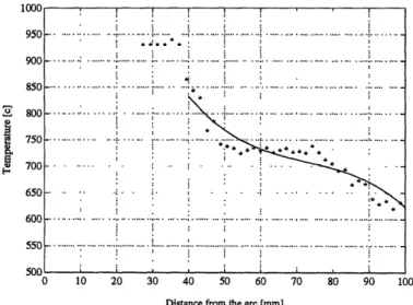
The calculation of cooling rate involves a derivative of the temperature distribution. Therefore a noisy temperature would give us a fluctuating measurement of the cooling rate. It is vital to remove as much noise as we can. Figure 2.1.4 shows an example of a measured temperature distribution of a weldment, where the noise is quite evident.

In order to eliminate the noise, temperatures are fit by a spline function composed of piece-wise third order polynomials.

The procedures for the fitting are as follows.

1. Temperatures are fit by a third order polynomial.

2. If the error of the fitting by the third order polynomial is greater than a specified value, the temperatures are fit by a spline function.

In order to reduce over-fitting, a third order polynomial is used as a basic function.

1UUU 950 900 850 % 800 750 700 650 600 550 Ann 0 10 20 30 40 50 60 70 80 90 100

Distance from the arc [mm]

' 3 I .. ... . " '. ' : : : - .. . . . . ... ... .... .. . .... : :. .. .. . _ .... ... ~~~~~~~~~~~~~~~.

., ....

(1) Fitting by third order polynomial

Figure 2.1.5 shows the fitting by a third order polynomial for the same data as shown in Fig. 2.1.4. In the figure the temperatures less than 600 °C are neglected, because they are so noisy that the fitting is aggravated. We can see the third order polynomial well fits the data.

h~ .4 10 95 90 85 80 75 70 65 60 55 ~ .. ... .. ... ... .. . .. ... ...

50 _

r*---

---

I--- -;-

--

e --

-

--- 0*

...

Distance from the arc [mm]

Fig. 2.1.5 Fitting by the 3rd order polynomial

100

(2) Fitting by spline function

The data shown in Fig. 2.1.4 are a typical steady-state temperature distribution. Steady-state temperatures can be fit well by a third order polynomial. However, if they are in the transient state it is sometimes hard to describe them as a third order polynomial. Figure 2.1.6 shows the fitting by a third order polynomial for a transient-state temperature distribution. We can see the

third order polynomial is not enough to fit these data.

U.. . ....i ...e. 950

900_,

-goo

...

Distance from the arc [mm]

Fig. 2.1.6 Fitting for transient-state temperature distribution

Such a temperature distribution should be fit by a higher order polynomial. However, it is known that a high order polynomial sometimes causes some fluctuations in its curvature. Another function which is often used is a spline function. A spline function, a continuous function that is composed of some piece-wise polynomials, is given by

f(x)

fi(k)(bi) = fi+(k)(bi) (k = 0 ... (m - 1)) (Continuity on nodes)

where fi (x) is the m-th order polynomial given by , aijx (i = 1 .. n), and bi denotes the nodes,

j=0

and then b=-oo,b = oo.

It is known that the spline function can be rewritten as:

m n-1

f(x)

=

zc

x'

+

d(x-bj)+

(2.1.4)

i=O j=1

xm ={0 (X <0) (Truncated m-th order polynomial) (2.1.5)

Therefore, the fitting by spline functions results in the estimation of the coefficient ci and dj,

which can be determined by the similar manner as the fitting by polynomials. The fitting by spline functions has the following good points:

1. It does not bring about fluctuations that are sometimes produced by a high order polynomial.

2. It is continuously differentiable.

Figure 2.1.7 shows the fitting by a spline function, which is composed of three third order piece-wise polynomials. We can see that it represents the temperatures well.

1000 950 . ... : ' " . .. : ... .... ...

900 ....

..

Distance from the arc [mm]

Fig. 2.1.7 Fitting by spline function

2.1.4 Other issues for measurement system

As shown in the figures above, the temperature is measured with respect to the location from the arc. Therefore, we need to know the location. The location is calculated geometrically from the angle of the mirror and the position where the mirror is situated. Since it is hard exactly to measure the position of the mirror, the relation between the angle of the mirror and the location where the pyrometer focuses is calibrated before experiment. To make the calibration, first a light source of a laser beam is mounted on the tube of the pyrometer. Then, the calibration data are obtained by observing the beam, and measuring the focused locations for some specified angles of the mirror.

To achieve a successful measurement of the temperature of the weldment, good alignment of the mirror and the pyrometer is crucial. In particular, the pyrometer should focus on the line of the weldment. We need check and adjust these devices by observing the laser beam so that the focal point will be located exactly on the line.

2.2 Measurement

Temperature gradient, cooling rate and location of critical temperature were observed during welding to see how the temperature distribution behaves for the step-wise change of travel speed and wire feed rate.

2.2.1 Measured variables

This section presents the definition of three variables, temperature gradient, cooling rate and location of critical temperature, and how to calculate them on-line. Before holding the discussion, we must keep in mind two types of coordinates for welding system. One is coordinates fixed to the workpiece, which will be called fixed coordinates. The other is coordinates fixed to the torch, called moving coordinates. The measurement is taken with respect to the moving coordinates. However, the definition of the cooling rate is based on the fixed coordinates. To avoid a confusion w is used as the location on the weldment with respect to the moving coordinates, and r denotes the location with respect to the fixed coordinates. T(w,t) implies the temperature of the time t with respect to the moving coordinates, while T'(r,t) is the temperature with respect of the fixed coordinates

t

Since r = v(t)dt+ r

+ w,

the relation between two representations of the temperature is given by

T(w,t) = T'(fv(t)dt + r + w,t) (2.2.l.a)

to

or T'(r,t) = T(-fv(t)dt- r + r,t) (2.2.1.b)

to

where r denotes the location of the torch at the initial time to, and v(t) is the velocity of the torch.

Temperature gradient

Temperature gradient Tg, the change of temperature per unit length at the critical temperature Tcr, is defined mathematically by

Tg(t) = _dT'(r,t)|

dr T=Trr, _ T(w,t)[

dw T=Tr

In the actual measurement, it is calculated by the following method:

To - AT

- dcr(t) -

dc,+a(t)

d,,(t) = arg{T(w,t) = T I

dr+AT(t) = arg{T(w,t) = (Ten + AT)

(2.2.3)

where d(t) denotes the location of critical temperature. The temperature gradient represents the spatial temperature change around the critical temperature.

Cooling rate

Cooling rate Cr, the change of temperature per unit time at the critical temperature, is given by

Cr(t) = dT'(rt)

dt T=Tr (2.2.4)

which is considered one of factors to represent the mechanical and metallurgical properties of the bead after welding. In steady-state this value is equivalent to the temperature gradient multiplied by the travel speed, because the temperature distribution in the moving coordinate is not dependent on time t, and the cooling rate is calculated as:

Cr

=

_ awl

F

dT(w)1

L dt j2 r L WJT=Tcr

= v Tg (2.2.5)

However, in the transient state it should be calculated as:

Cr = a 1 dT(w,t) 1 d _ T(w,t)

dL

L

\

t

The temperature gradient multiplied by travel speed is sometimes used as an alternative definition of the cooling rate. However, this definition brings about an unrealistic output in the transient state. For example, if the travel speed is abruptly changed, the cooling rate would also change abruptly, which is physically not possible.

The difficulty in the calculation of the cooling rate comes from the fact it involves the time and spatial derivatives, as shown in (2.2.6). Although various methods can be considered, the following will be used:

T(w,t - iAt) T(w,t)

N

CR(t)=argmin(AT -b) -a* i. At 2 (2.2.7) (Line -approximation) (2.2.7.a)

...

~~~~(2.2.7.a)

P

ai

=i(d,t;)-

cr

'=

~t

~- ~i.t

k~L~z.L.

/.D)

d.(t)

where v denotes the travel speed, and At is the sample interval. t' is the time when the past sample data was taken. In (2.2.7.c), d' implies where the location that presently has the critical temperature was located in the past temperature distribution T(w,t'). Therefore, AT_ishows how much the temperature drops from the time t' to the time t and reaches the critical temperature at the time t.

As shown above, we must use the present and past temperature distributions, which are usually contaminated by noise even if the temperature distributions are fit by spline functions to eliminate the noise. Therefore, if we calculate the cooling rate simply by ATl/At, the resultant data are quite fluctuating. To avoid this, the approximation shown in (2.2.7) is used.

Since the temperature drop AT is not proportional to the time difference (i. At), it is noted the measured cooling rate is not necessarily equal to the measured temperature gradient multiplied by velocity even in the steady-state due to the difference in the calculation methods of temperature gradient and cooling rate.

--11%_u

-" x, `

L'I-I

2.2.2 Measurement conditions

The variables above are measured for the following 4 cases:

Case A: Travel speed is kept constant at 4 mm/sec. Wire feed rate is changed from 18

cm/sec to 25 cm/sec as a step input.

Case B: Travel speed is kept constant at 8 mm/sec. Wire feed rate is changed from 18 cm/sec to 25 cm/sec as a step input.

Case C: Wire feed rate is kept constant at 18 cm/sec. Travel speed is changed from 4 mm/sec to 8 mm/sec as a step input.

Case D: Wire feed rate is kept constant at 25 cm/sec. Travel speed is changed from 4 mm/sec to 8 mm/sec as a step input.

The experiments were executed on mild steel, 12.7 mm thick and 60 mm in width under welding conditions of open-circuit voltage 30 v, Argon-2% oxygen shielding gas flowing at 100 I/min, and welding wire diameter 0.035 in.. The critical temperature is taken as 720 °C, given that the austenitization temperature is 727 °C.

2.2.3. Result of measurement

(1) The case where the travel speed is kept constant

Case A

Figure 2.2.1 shows the temperature gradient, the location of critical temperature, and the cooling rate for the case A, where the travel speed is 4 mm/sec and the wire feed rate is changed from 18 mm/sec to 25 mm/sec. The following results can be observed from this figure.

Temperature gradient

The temperature gradient gradually goes up form 9 °C/mm to 15 C/mm after the wire feed rate changes from 18 mm/sec to 25 mm/sec. After it reaches 15 mm/sec, it gradually goes down to the original point of 9 °C/mm.

Location of critical temperature

The location of critical temperature gradually moves away from the arc after the step input is given. It moves from 46 mm to 55 mm. After it reaches 55 mm, it is kept at this value.

Cooling rate

The cooling rate remains constant at about 40 °C/sec even if the wire feed rate is changed, although a distinct change in the temperature distribution can be seen from the responses of the temperature gradient and the location of critical temperature.

Some transient variation of the cooling rate after the step-wise change of the wire feed rate may take place, but be hidden in the noisy data. However, it is important to see that there would be no difference in the steady-state cooling rate before and after the step input. This result is also verified by the figure of the temperature gradient because the cooling rate in the steady-state is calculated as the temperature gradient multiplied by the travel speed. As mentioned above, the temperature gradient has the same value of 9 "C/mm in the steady-state before and after the step-wise change of the wire feed rate.

20 30 40 50 60

10 20 30 40 50 60

10 20 30 40 50 60

20 30 40 50 60

Fig. 2.2.1 Result of measurement for case A

t2i

Wire feedlrate [cm/sec]

20

10

-... ... -... ... .. -... .... .. ... . ... . .... .. ... .. ... ... ... ...

Travel speed [mm/sec]

i

10 U 4)0 S H~ 80 v 70 '; 60 o 50 40 f 30 ' 100 4 4 -50 U~. 3 10 -.U..- lL-.-. ^L~L~L· L --- ·. L-Y_ ~-_.·· L·L.·.-. -·.S * . . . ... ... ... ... ... ... ... ... ... . . .. ... .... . ... ... ... ...: ... ... ... ... ... ... ... ... ... ... ... ... . . ... . .... .. . .... ... . ... . ... .... .. """""""" """"""` """' "· ·""' '- · · · ·· · · ·~··· · · · ·· · · ·· · · ·~··· ... ... .... .··· Jv .... .. ... . .... ... ... . ... ... ... .... . .. .... ... . .... . ... ... ... . ... .... ... ... .. . ... .... .... .. . ... .... .... .... .. . ... .... . .. ... ... .... .. . . . . .. .. .. ... ... ... ... . .. ... .... . ... .... .. . . .. . .. . .. . . . .. . . . .. . . . .. . . . .. . .. . . .. . . . .. . . . .. . . .. . . . .

Case B

Figure 2.2.2 shows the results for the case B, where the travel speed is 8 mm/sec and the wire feed rate is changed from 18 mm/sec to 25 mm/sec. The following results similar to the case A are obtained from the figure.

Temperature gradient

It gradually goes up from 11 °C/mm to 15 °C/mm after the step-wise change of the wire feed rate. After it reaches the peek, it gradually goes down to the original point of 11

°C/mm.

Location of critical temperature

The location of critical temperatures gradually moves away from the arc after the step input. It moves from 47 mm to 53 mm. After it reaches 53 mm, it keeps the value.

Cooling rate

There is no distinct change in the cooling rate. It is kept around 130 °C/sec.

Comments on the cases where the travel speed is kept constant

1. It is clear that the heat input per unit time grows by the increase of the wire feed rate because the location of the critical temperature moves away from the arc after the increase.

2. The obvious increase of the width and height of the bead after the step input was observed in the experiments.

3. However, the cooling rate remains at almost same value.

4. Under the assumption that the heat input is proportional to the wire feed rate and the temperature is subject to the Rosenthal's model, the cooling rate should show about 38% increase.((25 - 18)/18 = 38%) However, the experiments show that is not the case.

10 15 20 25 30 10 15 10 15 20 20 25 25 30 30 10 15 20 25 30

Fig. 2.2.2 Result of measurement for case B Wire feed rate [cm/sec]

.... Trave sp... eed [m .... ... ... ... ... ... . ... s.... ... 20 10 0 Eo 15 0 1 5 80 , 70 '7 60 U 50 0 40 ' 30 o .atl l _· · _· · · _L_ LL_ L~_· *_I~___·~ _ L ·I _ _ _L I^^_ _ _·__·_ -... ,... ... ... ... ... !.. . ... . . . .. . . . .. . . .... . . . v -~~~~~~' ·~~~~~~~~~·~ ~ ~~~~ . .. .. .. . . .. .. .. .. . ... . . .. .. .. .. . . .. .. .. ... :...~~~~~~~~~~~~~~~~~~~~~~~~ .... .... .... .... .... .... .... 17_ nA

(2) The case where the wire feed rate is kept constant

Case C

Figure 2.2.3 shows the results for the case C, where the wire feed rate is 18 cm/sec and the travel speed is changed from 4 mm/sec to 8 mm/sec. The results are distinctly different from the case A and B.

Temperature gradient

The temperature gradient remains almost constant for a while after the stepwise change of the travel speed. It shows a sharp valley in its plot at almost same time when the location of the critical temperature shows a significant drop. The temperature gradient in the state shows a little change from 9 °C/mm to 11 °C/mm. This implies the steady-state cooling rate is almost proportional to the travel speed.

Location of critical temperature

The location of critical temperature shows a gradual increase from 48 mm to 65 mm after the change of the travel speed. When it reaches the peak, it suddenly decreases to the value of 45 mm and keeps the value. This sudden drop is quite different from the case of stepwise change of wire feed rate.

Cooling rate

The cooling rate does not show any significant variation for a while since we changed the travel speed. However, it suddenly increases in value from 40 °C/sec to 110 °C/sec 6 seconds later after the stepwise change. It shows a response involving a quite long delay and then a first order response with a short time constant.

10 15 20 25 30 35 40 45

10 15 20 25 30 35 40 45

15 20 25 30 35 40 45

Fig. 2.2.3 Result of measurement for case C

13n 10 AI _.. ... ... ... ... ... .. ...e ... . .a .. ... ... ... -..-...- ... ... ... .... ... ... ... . ... ... .... : ... ... ... ... a) '-4 bo a_ a) 0 -g_tW 0U 05 9:To I= c) o '-4 0 0 10 ill flu · ~ · _· l l . . ... .... ... ... .. ... ... . .... ... . .. .. ... . : · ·· · · ·· · · ·· · · ·. .... ... : .... ... · · · ·· · · ·· ·... ... . ... .. . .... .... .. .. ... . .. .... 200 150 100 50 0 -5o

Case D

Figure 2.2.4 shows the results for the case D, where the wire feed rate is 25 cm/sec and the travel speed is changed from 4 mm/sec to 8 mm/sec. The similar results to the case C are obtained.

Temperature gradient

Temperature gradient keeps the same value for about 5 seconds after the stepwise change of the travel speed. It shows a sharp valley in its plot. The temperature gradient in the steady-state shows a change from 8 °C/mm to 12 °C/mm.

Location of critical temperature

The location of critical temperature shows the gradual increase from 55 mm to 75 mm after the change of the travel speed. When it reaches the peak, it suddenly drops to the value of 49 mm and keeps the value.

Cooling rate

The cooling rate suddenly increases its value from 40°C/sec to 120 °C/sec 6 seconds later after the step input.

Comments on the case where the wire feed rate is kept constant

1. The heat input per unit time would be constant, because the wire feed rate is not changed.

2. The distinct decrease of the width and height of the weldment after the step input was observed in the experiments.

3. The step-wise change of the travel speed produces a time-delay and a first order

Wire feed rate [cm/sec]

l0 ~i... ..!... ... ... : ...

20 - . ... ... ... ... . ... ...

0 _{o10~ . ~Travel sped. [mm/.se}

10 15 20 25 30 35 40 45

20 ...

10 15 20 25 30 35 40 45

10 15 20 25 30 35 40 45

10 15 20 25 30 35 40 45

Fig. 2.2.4 Result of measurement for case D

2 I .__-, 6_w c

t

2.3. Remarks

1. Figure 2.2.5 shows the typical patterns of measured variables. First, these patterns show a distinct difference between the case where the wire feed rate is changed, and the case where the travel speed is changed. Of particular interest is the observation that the wire feed rate has little effect on the cooling rate, although a distinct change of the temperature distribution is observed. By contrast, the travel speed has a strong effect on cooling rate. This result suggests the cooling rate should be controlled by the travel speed, and can be controlled independently of mass transfer.

A_

Wire feed rate Travel speed

Fig. 2.2.5 Typical pattern of measured variables

2. Figure 2.2.6 shows the transient change of every one second in the temperature distribution for the case shown in Fig. 2.2.1, where the wire feed rate is changed from 18 cm/sec to 25 cm/sec. It performs as follows

a. After the step-wise change, the gradient of the temperature distribution becomes steeper from higher temperature. ( -(2))

b. After a while, the gradient is decreasing from lower temperature. ((2) - (3))

c. The final shape of temperature distribution, the steady-state shape, is almost same as the

I4 0a _, ;a '-4 o Ot -M a t5₀ A- 0 X . , ,,

I

U

4)

)0

Fig. 2.2.6 Change in temperature distribution by wire feed rate

3. To see more clearly the results of the steady-state cooling rate, let us consider the condition in which the cooling rate is not affected by wire feed rate, or heat input.

According to the principle of superposition, the steady-state temperature T(Q,w) can be written as

T(Q, w) = Qg(w) + To (2.3.1)

where Q is the heat input, and w is the distance from the arc, and Toare a constant. Then,

temperature gradient Tg is given by

Tg(Q,w) = -Qdg(w)/dwlTr

Since we are concerned with the critical temperature, T(Q, w) = T,, Then, (dQ/dw)g(w)r=r = -Qdg(w)/dwlT=r, the (2.3.2) (2.3.3) (2.3.4)

where dQ/dw shows the ratio between the change of the heat input and the location of the critical temperature which is caused by the heat input change.

We also have

dTg(Q,w)/dQ = -[dg(w)/dw + Q(d2_{g(w)/dw2 )(dw/dQ)]rT=T}

= - [dg(w)/dw - (d2g(w)/dw2)g(w)/(dg(w)/dw)lrT T In order that the steady-state cooling rate is not affected by the heat input,

dTg(Q, w)/dQ =

We can, therefore, get the condition: (dg(w)/dw)2 _{= (d}2_g(W)/dW2_)g(w)

, which results in the solution g(w) = A exp(aw) Therefore, T(Q,w) = QAexp(aw) + To (2.3.5) (2.3.6) (2.3.7) (2.3.8) (2.3.9)

More generally, we can write it as

T(Q, w) = f(Q)exp(aw) + To

by the similar discussion.

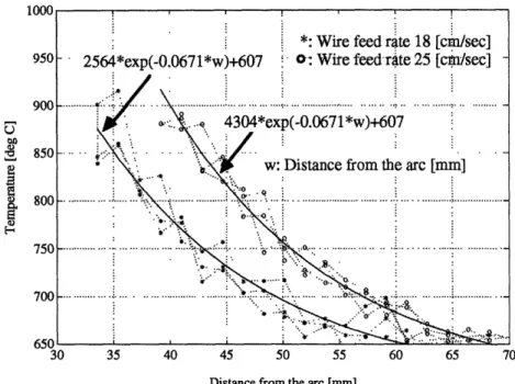
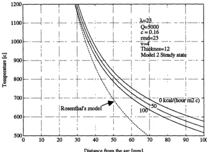
In Fig. 2.2.7 the steady-state temperature distributions obtained by the experiments are fit by an exponential function (2.3.9). It describes well the steady-state temperature distribution for the measurement range of 600 °C to 900 °C. The condition that the cooling rate is not affected by the heat input is satisfied.

IUUU

: Wire feed rate 18 [cm/sec]

950 - 2564*exp(-0.0671*w)+607 -o: Wire feedrate 25 [clsec]

9 0 0 ... '. ... ... .. .. ... . .. ...

V

4304*exp(-0.0671*w)+607

850 ... .

w:Distance from the arc [mm]

Xa2

80

...

m

' ... '

800

... ... ... ... : . ... ... .... . ... . .

700 . .. ....:: ...

30 35 40 45 50 55 60 65 70

Distance from the arc [mm]

Fig. 2.2.7 Steady-state temperature distribution (Travel speed 4 mm/sec)

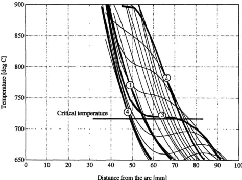
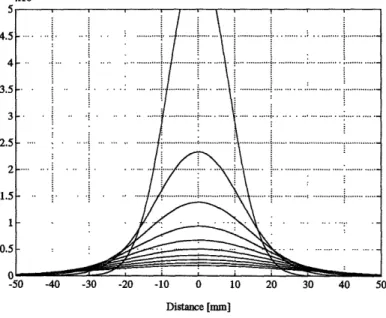
4. Figure 2.2.8 shows the change of every 500 msec in the temperature distribution for the case

shown in Fig. 2.2.4, where the travel speed is changed from 4 cm/sec to 8 cm/sec. The figure shows the following interesting characteristics.

a. After the step-wise change, the temperature distribution is shifting farther from the arc. (D -2)

b. After a while, it is decreasing its value from higher temperature. ((2) - (3 - ) c. The change from the state () to the state ) is quite fast. That yields the sudden

change of the temperature gradient, the location of the critical temperature and the cooling rate at the critical temperature.

---4)

a

4)

I)

Distance from the arc [mm]

Fig. 2.2.8 Change in temperature distribution

)0

by travel speed

5. The cooling rate must be determined in accordance with its metallurgical definition. The temperature gradient multiplied by the travel speed is sometimes used as an alternative. However, during the transient-state, its value is fairy different from the actual one, which would badly mislead the control system.

Chapter 3

Dynamic Model of Temperature Distribution

When we apply control to a process, we always have to evaluate the performance. The evaluation sometimes requires quite many experiments and adjustments of the parameters of the control. A model that describes the dynamic behavior of the process is used to reduce such laborious experiments and tuning of the parameters. It also gives us insight for designing the controller. In this chapter we study a model for this purpose. In particular we turn our attention to analytical models based on the heat conduction partial differential equation.

(Nomenclature)

The following nomenclature will be used throughout the chapter.

T(w,y,z,t) TO k

t

p

q(r),Q

a

= Initial temperature, Ambient temperature [°C] = Thermal diffusivity [m2/hour]

= Heat conductivity [kcal/(hour m °C)] = Time [hour]

= Specific heat [kcal/kg] = Density [kg/m3_]

= Scaled heat transfer coefficient [l/m]

= Heat transfer coefficient[kcal/(hour m2 °C)] divided by heat conductivity [kcall(hour m °C)]

= Heat input [kcal/hour] at time r, and constant heat input = Travel speed [m/hour]

= Location in the moving coordinate = Location in the fixed coordinate = Thickness [m]

3.1 Analytical models

The welding is a quite complicated process, which involves various phenomena such as heat conduction, heat convection, radiation, and mass transfer. The most important factor in the process is the heat conduction. However, we can not always neglect the other factors when we analyze the system. (Heiple et al. (1990)) Our concern lies in the cooling rate, which is a behavior after the solidification. Therefore, we focus our interest on heat conduction behavior.

Two types of models, an analytical model and a numerical model can be considered. However, the numerical model requires a large number of computations. That does not fit our purpose because we would like to evaluate the performance of the resulting controlled system by combining a controller with the model of the process. Therefore we use analytical models because they require fewer computations than numerical models.

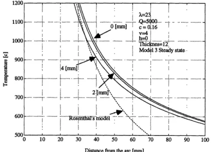
The analytical models under various given conditions are shown in the sequel. We can derive these models by using Green's function methods (Appendix A). Extensive derivation of the analytical models was done by Rosenthal (1946). Rosenthal's models have assumptions such as a point heat source and the neglect of a heat flux from the surface. Also these models only deal with a steady-state solution. Therefore, we can not see how the temperature behaves while the heat input and the travel speed are changing dynamically. For this problem, a Green's function method is very helpful. The first derivation of a model using Green's functions was by Edgar and Tsai (1983) to get a more general model under the assumption the heat has a Gaussian distribution. However,

(1) Semi-infinite steady-state model (Rosenthal)

Conditions

(a) Semi-infinite space (b) Point heat source

(c) No heat flux from the surface (d) Steady-state model

Model

T(w,y,z) = -exp(- r)exp(- - w) + To

2i A =r 2k 2k

r

= ~/w

y

(2) Model 1: Transient-state model under the same conditions as Rosenthal's model

Conditions

(a) Semi-infinite space (b) Point heat source

(c) No heat flux from the surface

Model 1 1 1 3q('r) T(wy,t)=jd4 ( )- exp(. 04 d[ ([-4t cp (w + v(1)dn)2 + y2 + z2 (

T

4k(t- )

T(w,y,z,t) = 1 pexp(_)

₁

3

exp(-)

.exp[

t-

(

-4k

dr+T

4(.j7_)

2k

(-t

--

_

,

z

(3.1.1)

1

lim T(w,y, z,t) -> Rosenthal' s model

t-.-(3) Model 2

Conditions

(a) Finite thickness, and infinite width and length (b) Point heat source

(c) Heat flux is described by:

LdT(w,y,z,t)

[dT(w, y,z,t) ) =-h(T(w,y,a,t)- TO)

(3.1.4) Transient-state model T(w,y,z,t) - T =

1

J[|

dr1

q(dr)

exp(

(w + v(ir)d)2 + y

4k(t-

:)

If the heat input and the travel speed are kept constant at Q and v, then

T(w,y,z,t) - T =

l_ _cp_ 2kV1 ) | t [ W2 +y 1 V2 2)(t

1Q oex

p

_(-

_{4k t-}

_-(741+

_kar

2

_)(t

_-

:

_)dn

_(z)an

_(O)

4 irk cp

2

t- expI--,

J

1Q=

Qexp(-

wv

)

exp

3'

D,

(z =

sin(az +fi)

a+

a,,

a+ 2,, = nr

tan(p,) = a

1 Q

exp

)

exps

2

-(4k

dsZIJI(z)~.(0)V

1

Q

WV)_ K

(4v

K0():The modified Bessel function of the second kind and zero order

(4) Model 3

Conditions

(a) Finite thickness, and infinite width and length (b) Gaussian heat source

q 1 W2 y2

Q(x,y,z)= q 1 exp(- )(z)

cp2r& 2 2₂

(c) Heat flux is given by the equation (3.1.4).

Transient-state model T(w,y,z,t)- To = (3.1.8) (3.1.9) (w+ v(rl)dn7)2 + y 2

4k(t- ) + 2 a2

- kax

_{(t - )]d,}

_(Z)n

₍₎

oo t

n 1 0 1

0=l