HAL Id: hal-02416666
https://hal.archives-ouvertes.fr/hal-02416666
Submitted on 21 Dec 2020HAL is a multi-disciplinary open access archive for the deposit and dissemination of sci-entific research documents, whether they are pub-lished or not. The documents may come from teaching and research institutions in France or abroad, or from public or private research centers.
L’archive ouverte pluridisciplinaire HAL, est destinée au dépôt et à la diffusion de documents scientifiques de niveau recherche, publiés ou non, émanant des établissements d’enseignement et de recherche français ou étrangers, des laboratoires publics ou privés.
Experimental and Theoretical Adsorption Study of
Ethanol on Ice Surfaces
N. Peybernès, Stéphane Le Calvé, Ph. Mirabel, S. Picaud, P. Hoang
To cite this version:
N. Peybernès, Stéphane Le Calvé, Ph. Mirabel, S. Picaud, P. Hoang. Experimental and Theoretical Adsorption Study of Ethanol on Ice Surfaces. Journal of Physical Chemistry B, American Chemical Society, 2004, 108 (45), pp.17425-17432. �10.1021/jp046983u�. �hal-02416666�
Experimental and theoretical adsorption study of ethanol on ice surfaces
N. Peybernès, S. Le Calvé * and Ph. Mirabel
Centre de Géochimie de la Surface / CNRS and Université Louis Pasteur, 1 rue Blessig, 67084 Strasbourg cedex, France.
S. Picaud and P.N.M. Hoang
Laboratoire de Physique Moléculaire - UMR CNRS 6624, Faculté des Sciences, 16, route de Gray, Université de Franche-Comté, 25030 Besançon Cedex, France.
Abstract
Adsorption study of ethanol on ice surfaces were performed by combining experimental and theoretical approaches. The experiments were conducted using a coated wall flow tube coupled to a mass spectrometric detection. The surface coverage increases with decreasing temperature and with increasing ethanol concentrations. The obtained experimental surface coverages were fitted according to the B.E.T. theory in order to determine the enthalpy of adsorption ∆Hads and the monolayer capacity NM: ∆Hads = - 57 ± 8 kJ mol-1, NM = (2.8 ± 0.8)×1014 molecule cm-2. The adsorption characteristics of ethanol on a proton disordered Ih(0001) ice surface were also jointly studied by performing classical molecular dynamics simulations. More specifically, the configurations of the molecules in their adsorption sites and the corresponding adsorption energies have been studied as a function of temperature and coverage. In the simulations, the saturation coverage is around NM = 3.2×10¹⁴ molecule cm-2, and corresponds to an adsorption energy equal to -56.6 kJ mol-1, in good agreement with the experimental value. The results are discussed and compared with previous determinations for alcohols.
* Corresponding author. Fax: +33-(0)3-90-24-04-02. E-mail address: [email protected]
Introduction
Recent measurements in the upper troposphere (UT) have revealed the presence of Partially Oxidised Hydrocarbons (POHs), such as alcohols, and these POHs may play an important role on the ozone cycle in this region. The upper troposphere defines a region of the atmosphere (between 8 and 12 km) characterised by its low temperatures (188 to 228 K) and where cirrus clouds cover a substantial portion (~25 %) of the earth's surface 1,2. Upper tropospheric air which has been transported from the warm boundary layer, may become highly supersaturated with respect to water or ice resulting in the formation of large number densities of ice particles 3. At temperatures below 233 K, cirrus clouds are predominantly composed of ice crystals 4 and these crystals can provide surfaces for trace gas interactions, that may promote heterogeneous reactions and therefore a re-partitioning of the different species between the gaseous and the solid phase.
The uptake of atmospheric pollutants on ice surfaces has been extensively studied for more than ten years, given their potential impact on the stratospheric ozone hole. Therefore, attention has mainly focused on halogenated or nitrated species such as HX, HOX, XONO2 (X = Cl, Br), N2O5 and HNO35-9. By contrast, very few articles have been devoted to the characterization of POHs on ice, although their photo-oxidation can provide a substantial source of HOx radicals that are involved in photochemical and chemical cycles leading to ozone loss in the atmosphere. Among these POHs, acetone on ice is certainly the system that has been the most experimentally studied10-14 and a relatively clear understanding of the acetone behavior on ice has emerged from the convergence of the various experimental data, in fair agreement with theoretical results15,16.
In a series of experiments, Sokolov and Abbatt have investigated the adsorption of different alcohols on ice as a function of their size (from ethanol to 1-hexanol)11, by using a coated-wall flow tube coupled to a mass spectrometer, between 213 and 245 K. The results show that the saturated surface coverages are all within ±50 % of 3.0×10¹⁴ molecules cm-2, and correspond to monolayer-like coverages for alcohols. These results also suggest that the alkyl chains are aligned perpendicular to the surface at monolayer coverage5,11. In order to characterize the influence of the organic function (C=O, O-H, C(O)OH, C(O)H) on the interaction between POHs and ice, the adsorption on ice of acetic acid11, formaldehyde12, methanol12,13, acetaldehyde13, and 2,3-butanedione14 has also been experimentally investigated, using a Knudsen cell flow reactor13 or a coated-wall flow tube11,12,14. The
corresponding adsorption energies have been measured within the same range, i.e. [-70, -50] kJ mol-1 for all these organic molecules except for formaldehyde, for which no significant adsorption has been evidenced.
From our knowledge, the theoretical studies devoted to the interaction between POHs and ice are very scarce. In a previous paper, we have used molecular dynamic simulations to characterize the adsorption of acetone on an ideal proton-ordered ice surface between 50 and 150 K15, and shown that this approach leads to theoretical results that are in good agreement with experimental data10-14, as well as with results issued from ab initio calculations at 0 K16. However, the main advantage of molecular dynamics simulations with respect to ab initio calculations is the inclusion of temperature effects, and the possibility of taking into account a large number of molecules in the simulation cell. These two characteristics allow calculations within the same temperature range and the same coverage conditions as in the experiments.
The goal of the present study is to re-examine the interaction of ethanol with ice surfaces, at temperatures relevant for the UT, with an approach that combines experiments and theory. Surface coverages of ethanol on ice have been experimentally measured in order to determine the values of the monolayer capacities NM and of the corresponding enthalpies of adsorption ∆Hads for temperature ranging from 193 K to 223 K. Our experimental data were then compared with those obtained in this work by Molecular Dynamics (MD) simulations performed in the same temperature range on a model proton-disordered ice surface. Although one previous experimental study has already been devoted to the ethanol/ice system11, this paper reports the first joint experimental and theoretical adsorption study of ethanol on ice.
Experimental section
The uptake of ethanol on ice surfaces was studied using a vertical coated wall flow tube (CWFT) coupled to a mass spectrometer, already described elsewhere 14. We will therefore provide only a brief summary of its principle operation. The apparatus, which is shown in figure 1, has a double jacket to allow the system to be operated at low temperature. The cooling fluid was circulated in the inner jacket from a cooler/circulator (Huber, Unistat 385) while vacuum was maintained in the outer jacket for thermal insulation. The temperature of the flow tube could be cooled down and regulated between 193 and 223 K.
The jacketed flow tube was approximately 40 cm in length with an internal diameter of 2.8 cm. The ice surface was prepared by totally wetting with Milli-Q water (18 MΩ cm) the inner wall of the flow tube that was typically precooled between 258 and 263 K. The water film was then rapidly cooled down to 253 K to form an ice film and then to the desired temperature over a period of 10-30 min. The thickness of ice film was estimated between 30 and 200 µm by weighting the resulting liquid water, when the ice film was melted at the end of the experiment.
The helium carrier gas (UHP certified to > 99.9995 % from Alphagaz) was used without further purification. During the experiment, water vapour was added to the main He flow in order to provide a partial pressure of water, equal to the vapour pressure of water over the ice film and therefore inhibit net evaporation of the ice film. In practice, a small fraction of the helium flow, varying typically between 1 and 5 mL min-1, was passed through a water bubbler thermostated at about 278 K and was diluted with a main flow of dry helium (100-200 mL min-1). The resulting gas mixture was then cooled down to the same temperature as that of the ice film in a glass tube of 20 cm in length (internal diameter 2.8 cm) where the excess of water was trapped. The resulting humidified helium flow was injected at the upstream end of the flow reactor.
Ethanol (≥ 99.8 %) was purchased from Carlo Erba and was further purified before use by repeated freeze, pump, and thaw cycles as well as by fractional distillation. To perform an experiment, ethanol was then premixed with helium in a 10 L glass light-tight bulb to form 1.1×10⁻² – 2.4×10⁻¹ % mixtures, at a total pressure of ≈ 800 - 950 Torr. The mixture containing ethanol was injected into the flow tube reactor via a sliding injector (figure 1). This later permits to change the reaction distance which can be varied up to 40 cm in order to change the gas/ice interaction time (0 - 700 ms) or the exposed ice film surface (50 - 260
cm2). The injector was jacketed and a heating tape was wound up in the jacket, to ensure a gentle heating of the injector 14.
All the gases flowed into the reactor through Teflon tubing. The gas mixture containing ethanol and water vapour diluted in helium was flowed through the reactor with a linear velocity ranging between 60 and 120 cm s-1. The concentrations of ethanol in the gas phase were calculated from their mass flow rates, temperature and pressure in the flow tube (CWFT). All the flow rates were controlled and measured with calibrated mass flowmeters (Millipore, 2900 series) and the pressure that ranged between 2.5 and 7.0 Torr, was measured with two capacitance manometers (Edwards, 622 Barocel range 0-100 torr and Keller, PAA-41 range 0-76 torr) connected at the top and bottom of the flow tube. Under our experimental conditions, the mixing time τmix between ethanol flow and the main He flow was lower than 2 ms 15 which corresponds to a mixing length smaller than 0.3 cm.
The gas stream coming out of the flowtube was analysed using a differentially pumped mass quadruple spectrometer Pfeiffer Vacuum QMS. Ethanol was monitored at the parent ion C2H5(O+)H peak at m/z = 46 amu, using a temporal resolution of 60 ms, an ionisation energy of 70 eV and an emission current of 1000 µA.
Experimental Results
Our work is the second experimental study of adsorption of ethanol on ice surfaces 11. Uptake experiments were performed by first establishing a highly stable flow of ethanol in the injector, this injector being positioned past the end of the ice film. The injector was then moved quickly (at ≈ 45 s, see figure 2) to an upstream position so that the ice film is exposed to ethanol. The uptake of ethanol on the ice film leads to a drop of signal as shown in figure 2. On a time scale of about 15 s, the surface became saturated and the MS-signal returned to its initial level. When the injector was pushed back (t ≈ 124 s), the ethanol molecules desorbed from the ice surface and the signal increased and then again returned to its initial level after 15 s. Similar experiments were conducted over a temperature range 193 – 223 K and for gas phase concentrations of ethanol varying from 6.4×10¹¹ to 1.2×10¹³ molecule cm-3.
In the temperature range of 203-223 K and for concentrations mentioned above, the integrated areas of the adsorption and desorption peaks were found to be the same, within experimental errors, so that adsorption of ethanol on ice could be considered reversible. Similar reversible adsorptions on ice were already observed for acetone, methanol and formaldehyde by Winkler et al. (2001) 12 or for C2-C6 n-alcohols by Sokolov et al. (2002) 11.
At 193 K and for concentrations larger than 7×10¹² molecules cm-3, the desorption peak was significantly smaller than the adsorption peak. As observed for the uptake of many species on ice surfaces 17,18, unlimited gas-phase uptake can occur at low temperature and high gas phase concentrations due to a mechanism of surface adlayer growth via a flux of both ethanol and water vapor to the ice surface to generate a liquid solution or amorphous supercooled mixture. The missing ethanol will then be trapped either inside the generated solution or under this latter in the first solid layers.
Surface coverage
The number of ethanol molecules adsorbed on the ice surface was determined from the integrated area of the adsorption peak (in molecule s cm-3) and the total flow rate in the flow tube (cm3 s-1). The surface coverage N (in molecule cm-2) of ethanol on ice was then calculated from the exposed ice surface Sice (in cm-2) according to N = Nads/Sice where Nads is the number of ethanol molecules adsorbed on the exposed ice surface. Our experimental ice surface areas are considered equal to the geometric areas of pyrex.
The experiments were performed using 5 different diluted mixtures and 8 newly generated ice surfaces in order to verify the reproducibility of the data. A typical example of ice film is shown in figure 3. The plot of surface coverage N versus the gas phase concentration at 223 K is shown in figure 4, together with the results obtained by Sokolov and Abbatt 11. The relative errors on the gas phase concentrations (horizontal error bars) calculated from the possible uncertainties on each flow, total pressure etc. range between 2 and 25 %. The quoted errors on N (vertical error bars) arise from uncertainties made on the total flow rate, on the exposed ice area, on the concentration in the gas phase. They also include a systematic error of 2 % that corresponds to the error on the integrated area of adsorption peak. The resulting error on N varies between 6 and 20 %.
Isotherms
In this work, the data have been fitted by using B.E.T. isotherm theory where the surface is considered uniform so that all sites are equivalent and the ability of a molecule to adsorb at a given site is independent of the neighbouring sites. The choice for this quite simple model has been a posteriori justified by the very good comparison between the results issued from these experiments and those issued from molecular dynamics simulations (see the theoretical part of this paper). In B.E.T. model, the initial adsorbed layer can act as a substrate for further
adsorption. In this case, for all layer except the first, the heat of adsorption is equal to the molar heat of condensation L.
The most convenient form of the BET equation for application to experimental data is given by the following equation:
0 M M 0 0 p p C N 1 C C N 1 )) p / p ( 1 ( N p p Y ⋅ ⋅ − + ⋅ = − = (1)
where Y is the BET function 19, p and p0 are respectively the partial pressure of the compound in the flow tube and its saturation pressure (Torr) and C is the BET constant (no unit). The values of the saturation pressures p0 were calculated from the Antoine equation:
c T b a p log 0 + − = (2)
The Antoine parameters available in the literature for ethanol are a = 5.372, b = 1670.41 and c = -40.19 20. The saturation vapour pressures of ethanol are then the following (in Torr): 2.07×10⁻³ (193 K); 9.71×10⁻³ (203 K); 3.81×10⁻² (213 K); 1.29×10⁻¹ (223 K).
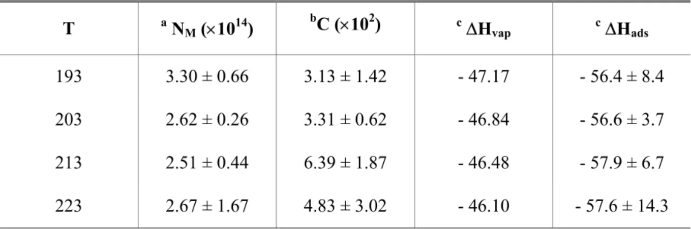
The plot of Y against p/p0 gives a straight line with a slope s = (C-1) / NM C and an intercept i = 1 / NM C. The BET plot is linear for relative pressures higher than 7.5×10⁻⁴ as shown in figure 5. The values of NM and C determined from a combination of the slope and intercept (NM = 1/(s+i) ; C = s/i + 1) are reported in table I. The B.E.T. constant is then used to derive the enthalpy of adsorption from the following expression:
(T) H lnC RT (T) Hads =− +∆ vap ∆ (3)
The enthalpy of adsorption is independent of temperature between 193 and 223 K and the average value is ∆Hads = – 57 ± 8 kJ mol-1. Even if the values of NM seem to be slightly higher for the lowest temperature (193 K), the average monolayer capacity corresponding to the adsorption of ethanol on ice surfaces is NM = (2.8 ± 0.8)×1014 molecules cm-2. For either ∆Hads or NM, the quoted uncertainties were taken as the mean of the four individual errors at each temperature.
Comparison with previous studies
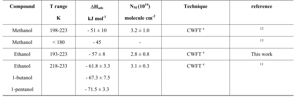
Our results are reported in the table II together with previously reported data for primary alcohols RCH2OH (where R = H, CH3, C2H5, n-C3H7). Sokolov and Abbatt (2002) 11 have studied the adsorption of ethanol on ice surfaces between 218 and 233 K in the concentration range of 3.01×10¹¹ - 2.73×10¹³ molecules cm-3, using a Coated Wall Flow Tube coupled to a mass spectrometer. Under their experimental conditions, the adsorption was always found reversible. In the figure 4, our measurements of N (molecules cm-2) plotted versus the concentration of ethanol at 223 K, are in good agreement with those determined by Sokolov and Abbatt. In the same way, our values of NM and ∆Hads are also consistent with those derived by these authors with Langmuir model: NM = 2.9×10¹⁴ molecules cm-2, ∆Hads = – 61.8 ± 3.3 kJ mol-1.
The same authors have shown that the monolayer capacity of a primary alcohol on ice do not change within the experimental errors (NM = 3.1×10¹⁴ molecules cm-2) when the alkyl chain increases. They concluded that it was probably an indication that when the surface is saturated, the molecules are oriented in a similar manner with the hydroxyl group binding to the ice surface and the alkyl chain at right angles to the surface. They have also found that the adsorption enthalpy decreases in absolute value when the alkyl chain was shorter. Indeed, the value of ∆Hads = – 61.8 ± 3.3 kJ mol-1 for ethanol is smaller in absolute value than that for 1-butanol (∆Hads = – 67.3 ± 7.5 kJ mol-1), itself lower than that obtained for 1-pentanol (∆Hads = – 71.5 ± 3.3 kJ mol-1) 11. This is consistent with the both determinations of ∆Hads for methanol: ∆Hads = – 51 ± 10 kJ mol-112and ∆Hads = – 45 kJ mol-113.
Molecular dynamics calculations Interaction potential
The intermolecular potentials used in the present study to describe the interaction between water and ethanol molecules consist of site-site potentials which contain coulombic and Lennard-Jones contributions. These potentials are written as
) r ( V ij σ − σ ε + = 6 ij ij 12 ij ij ij 2 ij j i ij r r 4 e r q q ) r ( V (4)
where is the distance between the ith and jth sites of the interacting molecules. qrij ie is a point charge located at the ith site, and ε, are the usual Lennard-Jones parameters. For the σ lateral interaction V between the ethanol molecules, we use the model proposed by Briggs et al.
eth eth−
21 in which charges and dispersion-repulsion centers are located on the atoms of the hydroxyl group and on the C atom of the alkyl groups, that are treated as single sites centred on the carbon atom. TIP4P model is used for water-water interaction22 ( ) and the parameters for the interaction V between ethanol and water are obtained by using the usual Lorentz-Berthelot combining rules, defined as follows:
w w V − w eth− j i ij ε ε ε = (5) and 2 j i ij σ σ σ = + (6)
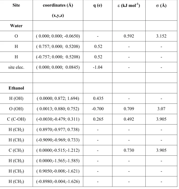
The various potential parameters are summarized in Table III. In the simulation, all interactions between sites are damped through a switching function S(R) (where R is the centers of mass separation between molecules) which is defined such as, at the boundaries of the switching region, the potential energy is continuous and the switching function first and second derivatives are zero15.
Details of the simulation
We consider adsorption on the (0001) basal plane of proton disordered hexagonal ice. The simulation box is a parallelepiped of sizes Lx = 35.914 Å and Ly = 38.878 Å along the x and y directions perpendicular to the c axis of ice. It contains six bilayers of moving water molecules which form a slab of 21.99 Å thick. These moving water molecules are placed on a slab consisting of four bilayers of fixed water molecules. To simulate an infinite surface, periodic boundary conditions are imposed by replicating the simulation box along (x,y). This box contains a total of 1600 water molecules, 960 of them being moving molecules. The initial configuration of the water molecules23 obeys the ice rules24 and has no net charges and no net dipole moment. In order to check the influence of the proton ordering on the simulation results, we have also considered adsorption on proton ordered hexagonal ice. In this case, the simulation box is a parallelepided of sizes Lx =4lx, Ly =4ly, based on an orthorhombic unit cell of sizes lx =8.98Å, Å and ly =7.78 lz =7.33 Å. This unit cell contains 8 water
molecules. Periodic boundary conditions are imposed by replicating the unit cell along the x and y directions, and the simulation box contains 960 moving molecules forming a slab of thickness Lz =4lz (along the z direction), adsorbed on 640 fixed water molecules (Fig. 6).
The simulation box also contains a certain number of moving ethanol molecules that is determined from experimental results. In the experiments, the averaged maximum number of adsorbed ethanol molecules in a monolayer is equal to (2.8 ± 0.8)×1014 molecules.cm-2 (see experimental section). This corresponds to 45 13± molecules in our simulation box. Thus simulations have been performed at low (9 ethanol molecules), medium (25 and 49 ethanol molecules) and high coverages (64 and 98 ethanol molecules). At the beginning of the simulations (initial conditions), the ethanol molecules are randomly distributed above the surface, in a single plane (9, 25, 49 and 64 molecules) or in two planes (98 molecules) because, on the basis of the experimental results, this latter coverage would correspond to the formation of more than one monolayer above the ice surface.
Each molecule is treated as a rigid rotor, and six external coordinates are used to describe the translation of the center of mass (x,y,z) and the orientation of the molecule ( ) with respect to an absolute frame tied to the bottom of the simulation box. The translational equations of motion are solved with a time step of 2.2 fs using the Verlet algorithm, and a predictor-corrector method based on the quaternion representation of the molecular orientations is used for the orientational equations
χ θ ϕ ,,
25. Every run involved an equilibration period of 60000 steps (132 ps), followed by a production run of 40000 steps (88 ps). The initial linear and angular velocities for each moving molecule are taken from a Boltzmann distribution corresponding to the desired simulation temperature. The simulations are performed in the NVT ensemble using a Berendsen thermostat. The potential cut-off in the calculations of the acetone-acetone, acetone-water and water-water interactions is handled through three different neighbor lists25, with the same radial cutoff (15 Å) in the direct space. Due to this large cut-off, the calculations of the electrostatic interactions through the Ewald scheme were not necessary26. Simulations are performed at 193 and 223 K, i.e. the boundaries of the temperature range considered in the experiments.
Theoretical Results
Geometry of the admolecules
We first characterize in our calculations the translational ordering of the ethanol molecules along the z axis, perpendicular to the ice surface, in order to determine the
maximum coverage corresponding to the formation of one complete monolayer above the ice surface. Indeed, this information can be directly compared to the experimental data.
As an example, the distribution functions p(z) of the distances between the molecular centers of mass of the moving molecules (water + ethanol) and the origin of the absolute frame is given in Fig. 7a for a coverage of 49 ethanol molecules, at both 193 and 223 K. The double peaks correspond to the hexagonal arrangement of the water molecules, which is preserved at these low temperatures, although a certain disorder is evidenced for the surface layer of the ice crystal. Note that these distribution functions for the water molecules are very similar to those obtained by Kroes in molecular dynamics simulations of the surface melting of the (0001) face of TIP4P ice (i.e. using the same potential than in the present simulations)27, indicating that the ethanol adsorption between 193 and 223 K does not significantly modify the ice surface characteristics. At the surface of our ice crystal, the single peak around 36.0 Å corresponds to the monolayer arrangement of the 49 ethanol molecules. This peak does not shift significantly when the temperature increases from 193 to 223 K, although it slightly broadens due to the thermal fluctuations (Fig. 7a).
The distribution functions p(z) at 193 K for the ethanol molecules only are also shown in Fig. 7b in order to study the influence of the ethanol coverage on the translational ordering of the adsorbed molecules. In this figure, it is cleary evidenced that two layers are formed for the highest coverage (98 molecules) since two peaks are obtained in the corresponding p(z) function. The integrals of these peaks indicate that the layer close to the ice surface contains 64 ethanol molecules, whereas the 34 remaining molecules arrange themselves in a second layer. Lower ethanol coverages lead to the occurrence of only one peak in p(z) (Fig. 7b), indicating the formation of a single ethanol layer above the ice surface. However, it is interesting to note that, in the simulation with 64 molecules (i.e. the number of molecules corresponding to the monolayer completion in the simulation with 98 molecules), only 55 molecules out 64 are arranged in a first layer, the remaining molecules being adsorbed in an upper layer (Fig. 7b). This difference is due to the fact that, in a simulation with 98 molecules, the 34 excess molecules in the upper layer act as a cover that prevents the 64 molecules in the lower layer from escaping.
On the basis of these results, we can conclude that, from a theoretical point of view, the monolayer contains between 49 and 55 molecules, i.e. between 3.0 and
molecules.cm
14
10 4 .
3 × -2. Similar results are obtained when considering the proton-ordered ice crystal.
Additional information concerning the orientations of the ethanol molecules can be obtained from the simulations, through the study of the angular distribution functions p(θ , )
, of the Euler angles , , and )
(
p ϕ p(χ) θ ϕ χ that represent the orientation of the molecule in an absolute frame. defines the orientation of the C—C axis with respect to the z axis perpendicular to the ice surface, is the angle made between the projection of this C—C axis in the (x,y) plane and the y axis, and the internal rotation of the ethanol molecule around its C—C axis is characterized by . The angular distribution functions are given in Fig. 8 for two typical situations corresponding to submonolayer (9 molecules) and (nearly) monolayer (49 molecules) coverages, at 193 K. At submonolayer coverage, the distribution exhibits a single large peak around 115°, with a full width at medium height (FWMH) equal to about 30°. This value corresponds to a tilted orientation of the C—C axis of the ethanol molecules, the methyl group being away from the ice surface. Note that the large value of the FWMH indicates large angular fluctuations around the mean value, due to the thermal motions at the temperature of the simulation. In the same way,
θ ϕ χ ) ( p θ ) (
p χ is characterized by one single large peak centered around a mean value of 300° which corresponds to an orientation of the OH group directed toward the ice surface, compatible with the formation of hydrogen bonds with the water molecules. At full monolayer coverage, additional peaks are evidenced in p(θ and )
due to lateral interactions which tend to flatten down ( )
(
p χ θ 83= °) or to lift up ( )
the ethanol molecules. However, a careful analysis of the data shows that the molecular orientations still correspond to a configuration where the OH groups are closer to the ice surface than the alkyl chains (see Fig. 9).
° 150 = θ
The distribution function p(ϕ) (not shown) is much less structured than p(θ) and p(χ ) and tends to spread over the whole angular range. This feature is connected to the proton disordering at the ice surface and to the optimization of the lateral interactions between ethanol molecules.
Very similar results are obtained at 223 K, although the corresponding peaks in the orientational distribution functions are wider due to larger thermal fluctuations. By contrast, more pronounced preferred orientations are obtained on proton ordered ice (not shown), due to the periodic arrangement of the dangling OH bonds at the ice surface.
Energy of the admolecules
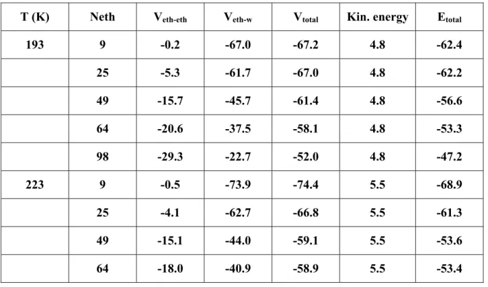
The different contributions to the total energy for the system ethanol-proton disordered ice are given in Table IV. At 193 K, and low coverage (9 ethanol molecules), the lateral interactions between ethanol molecules ( ) are negligible, and the total potential energy (about -67 kJ mol eth eth V − eth eth V − w eth−
-1) mainly comes from the electrostatic interaction between ethanol and water molecules. When the coverage is increased up to the completion of one monolayer (between 49 and 64 ethanol molecules), increases from 8% (25 ethanol molecules) to 26 % (49 ethanol molecules) and 35 % (64 ethanol molecules) of the total potential energy. Note that the ethanol-ice interaction ( V ) decreases (in absolute value) when increasing the ethanol coverage due to the influence of the lateral interactions on the geometry of the adsorbed ethanol molecules. This leads to a strong decrease of the total energy when a second layer of ethanol is formed above the ice surface (98 ethanol molecules).
Taking into account the kinetic energy, the total energy per ethanol molecule ranges from -47.2 to -68.9 kJ mol-1 for the various coverages and temperatures considered in the present simulations.
Very similar trends are obtained when considering adsorption on proton-ordered ice crystal. Indeed, around monolayer coverage, the total energy at 193 K increases from -53.0 to -51.7 kJ mol-1 when the coverage is increased from 49 to 64 ethanol molecules in the simulation box, respectively.
Characterization of hydrogen bonds
In order to characterize the hydrogen bonding between ethanol molecules and ice, and between neighbouring ethanol molecules, we have calculated pair radial distribution functions corresponding to distances between H and O atoms of the different partners. Three typical functions are given in Fig. 10 for the ethanol monolayer (49 molecules) at 193 K; two of them ( and g ) represent the probability of finding an H or an O atom of the hydroxyl group of an ethanol molecule at a distance r from an O or an H atom of the water molecules of the ice surface, respectively; the last one ( g ) characterizes the probability of finding H and O atoms of hydroxyl groups of two neighbouring ethanol molecules a distance r apart. These three functions mainly exhibit a strong peak centred around 1.8 Å that, on the basis of the O H—O distance criterion, is compatible with the
) r ( gHe−Ow Oe−Hw(r) ) r ( He Oe− L
formation of hydrogen bonds. The integrated intensity of the first peak in g , up to the first minimum, gives the number of Y atoms in the first shell of the X atom. The present results for and g indicate that 55 % of the ethanol molecules act as a proton donors, whereas 42 % of these molecules acts as proton acceptors, the remaining molecules (around 3 %) being not involved in such bonding with the ice surface. For the third function ( ), the integrated intensity of the first peak indicates that, in average, 43 % of the ethanol molecules are also bound via lateral hydrogen-bonds. Note that some ethanol molecules form hydrogen-bonds both with the ice surface and with a nearest neighbour ethanol molecule, as shown on the snapshot issued from the simulation at 193 K and at monolayer coverage (49 molecules, Fig. 9).
) r ( Y X− ) r ( gHe−Ow ) r ( He Oe− ) r ( Hw Oe− g Conclusion
The present paper reports the first combined experiments/theory study of the interactions between ethanol and ice. In the experiments, the adsorption of ethanol on ice has been characterized between 193 and 223 K, and is found to be (almost) fully reversible in this temperature range. The enthalpy of adsorption is independent of temperature between 193 and 223 K, and the average value is ∆Hads = – 57 ± 8 kJ mol-1. Even if the values of NM seem to be slightly higher for the lowest temperature (193 K), the average monolayer capacity corresponding to the adsorption of ethanol on ice surfaces is NM = (2.8 ± 0.8)×1014 molecules cm-2. These values are in good agreement with previous experimental data11. From a theoretical point of view, molecular dynamics simulations have been used to investigate, at a molecular level, the details of the adsorption characteristics of ethanol on ice, in the same temperature range as in the experiments, and with a number of ethanol molecules in the simulation box that reproduces the experimental amount of adsorbed molecules. At first sight, it seems quite difficult to compare the theoretical results with the experimental data because the simulations are performed on a perfect ice crystal, and correspond to equilibrium situations. Nevertheless, the energy values obtained in our simulations are in very good agreement with the measured values, and this indicates that the potential used in the present study is accurate enough to describe the ethanol/ice interactions. This also justifies a posteriori our analysis of the experimental data with the BET theory. Note that no other theoretical study is available in the literature for the ethanol/ice system. The calculated saturation coverage (3.2×10¹⁴ molecules.cm-2) is also in good agreement with the values
issued from the BET analysis of the experimental data, and is similar to that deduced from experimental and theoretical studies of other systems such as methanol or acetone adsorbed on ice11-13,15,16. The main advantage of the simulations is that they provide additional information on the structure of the adsorbate, and on the competition between ethanol-ice and ethanol-ethanol interactions. In particular, the theoretical results evidence the formation of hydrogen bonds in the simulated system, and a relatively strong influence of the intra-adsorbate interactions on the structuration of the ethanol molecules on ice. Finally, the present simulations indicate that the ethanol molecules are oriented with their alkyl chain directed away from the ice surface (Fig.9), in agreement with the trends inferred from experiments on alcohols of different sizes adsorbed on ice11.
Acknowledgement
This work was supported by EC (project CUT-ICE, EVK2-CT1999-00005) and by CNRS (program PNCA). This is the EOST contribution n° 2004.XXX-UMR7517.
References
1 Solomon, S.; Borrmann, S.; Garcia, R. R.; Portmann, R.; Thomason, L.; Poole, L. R.; Winker, D.; McCormick, M. P., J. Geophys. Res., 1997, 102, 21411.
2 Winkler, D. M.; Trepte, C. E., Geophys. Res. Lett., 1998, 25, 3351.
3 Wang, C.; Crutzen, P. J.; Ramanathan, V.; Williams, S. F., J. Geophys. Res., 1995, 100, 11509.
4 Heymsfield, A. J.; Sabin, R. M., J. Atmos. Sci., 1989, 46, 2252. 5 Abbatt, J. P. D., Chem. Rev., 2003, 103, 4783.
6 Hanson, D. R.; Ravishankara, A. R., J. Phys. Chem., 1992, 96, 2682. 7 Chu, L. T.; Leu, M. T.; Keyser, L. F., J. Phys. Chem., 1993, 97, 12798.
8 Tabazadeh, A.; Toon, O. B.; Jensen, E. J., Geophys. Res. Lett., 1999, 26, 2211. 9 Kroes, G. J., Comments At. Mol. Phys., 1999, 34, 259.
10 Schaff, J. E., Roberts, J.T., Langmuir, 1998, 14, 1478.
11 Sokolov, O.; Abbatt, J. P. D., J. Phys. Chem. A, 2002, 106, 775.
12 Winkler, A. K.; Holmes, N. S.; Crowley, J. N., Phys. Chem. Chem. Phys., 2002, 4, 5270.
13 Hudson, P. K.; Zondlo, M. A.; Tolbert, M. A., J. Phys. Chem. A, 2002, 106, 2882. 14 Peybernès, N.; Marchand, C.; Le Calvé, S.; Mirabel, P., Phys. Chem. Chem. Phys.,
2004, 6, 1277.
15 Picaud, S.; Hoang, P. N. N., J. Chem. Phys., 2000, 112, 9898. 16 Marinelli, F.; Allouche, A., Chem. Phys., 2002, 272, 137.
17 Barone, S.; Zondlo, M. A.; Tolbert, M. A., J. Phys. Chem. A, 1999, 103, 9717.
18 Hudson, P. K.; Shilling, J. E.; Tolbert, M. A.; Toon, O. B., J. Phys. Chem. A, 2002, 106, 9874.
19 Gregg, S. J.; Sing, K. S. W., Adsorption, Surface Area and Porosity; second edition ed.; Academic Press Inc.: San Diego, 1982.
20 NIST, www.webbook.nist.gov/chemistry.
21 Briggs, J. M.; Nguyen, T. B.; Jorgensen, W. L., J. Phys. Chem., 1991, 95, 3315. 22 Jorgensen, W. L.; Chandrasekhar, J.; Madura, J. F.; Impey, R. W.; Klein, M. L., J.
Chem. Phys., 1983, 79, 926.
23 Buch, V.; Sandler, P.; Sadlej, J., J. Phys. Chem. B, 1998, 102, 8641.
24 Eisenberg, D.; Kauzmann, W., The Structure and Properties of Water: Clarendon: Oxford, 1969.
25 Allen, M. P.; Tildesley, D. J., Computer Simulations of Liquids: Clarendon: Oxford, 1987.
26 Spohr, E., J. Chem. Phys., 1997, 107, 6342. 27 Kroes, G. J., Surf. Sci., 1992, 275, 365.
Figure captions
Figure 1: Schematic illustration of the vertical coated wall flow tube.
Figure 2: Ethanol concentration in the gas phase as a function of time during the adsorption of ethanol on ice surfaces at 213 K with [ethanol] =4.6×10¹² molecule cm-3.
Figure 3: Digital picture of a typical ice film (74 µm). Note that the stripes correspond to the winding of the resistance around the warming and sliding injector (in white).
Figure 4: Surface coverage of ethanol versus its gas phase concentration at 223 K. Our data are compared with those obtained by Sokolov and Abatt (2002). Our quoted errors are detailed in the text.
Figure 5: Plot of Y versus the relative pressure (p/p0) according to the B.E.T. model (see eq. 1) for the four studied temperature i.e. 193, 203, 213 and 223 K. The dashed line represents the lower limit under which B.E.T. analysis is not valid i.e. for p/p0 < 7.5×10⁻⁴ while the solid lines correspond to the plots obtained according to eq. 1. The quoted errors are detailed in the text.
Figure 6: Snapshot of the ice crystal (side view of the simulation box) at T = 193 K, showing the six mobile layers of proton disordered ice adsorbed on four rigid ice layers.
Figure 7: (a) Distribution functions p(z) (in arbitrary unit) of the distance z (Å) of the water and ethanol molecular centers of mass from the bottom of the simulation box at 193 and 223 K for a coverage equal to 49 ethanol molecules; (b) distribution functions p(z) of ethanol molecules only, for different coverages at 193 K, and for proton disordered ice.
Figure 8: Angular distribution functions for the ethanol molecules on proton disordered ice at 193 K and for two typical coverages : nearly isolated molecules (9 molecules – dotted curve) and monolayer (49 molecules – full curves): (a) angle θ; (b) angle χ. The angles are in degrees, and the distribution functions are given in arbitrary units.
Figure 9: Snapshot issued from the simulation of 49 ethanol molecules adsorbed on proton disordered ice ((a) top view; (b) side view showing only the top layers of the system) at 193 K. The water molecules are represented by small sticks for clarity.
Figure 10: Radial distribution functions g(r) for the distances between the oxygen atom of the ethanol molecule and the H atoms of the water molecules ( ) or the H atom of the OH group of the neighboring ethanol molecules ( g ), and between the hydrogen atom of the OH group of the ethanol molecule and the O atom of water ( g ), at 193 K and for a coverage corresponding to 49 ethanol molecules on proton-disordered ice.
) r ( gOe−Hw He ) r ( He Oe− ) r ( Ow −
Table I: Fit parameters for B.E.T. Isotherms corresponding to adsorption of ethanol on ice surfaces. The errors bars are given at 2σ levels (see text).
T a NM (×1014) bC (×102) c∆Hvap c∆Hads
193 3.30 ± 0.66 3.13 ± 1.42 - 47.17 - 56.4 ± 8.4 203 2.62 ± 0.26 3.31 ± 0.62 - 46.84 - 56.6 ± 3.7 213 2.51 ± 0.44 6.39 ± 1.87 - 46.48 - 57.9 ± 6.7 223 2.67 ± 1.67 4.83 ± 3.02 - 46.10 - 57.6 ± 14.3
Table II: Adsorption of ethanol on ice surfaces: comparison with previous works. Compound T range K ∆Hads kJ mol-1 NM (1014) molecule cm-2 Technique reference Methanol 198-223 - 51 ± 10 3.2 ± 1.0 CWFT a 12 Methanol < 180 - 45 - 13
Ethanol 193-223 - 57 ± 8 2.8 ± 0.8 CWFT a This work
Ethanol 1-butanol 1-pentanol 218-233 - 61.8 ± 3.3 - 67.3 ± 7.5 - 71.5 ± 3.3 3.1 ± 0.3 CWFT a 11
Table III: Parameters for the potentials used in the simulations. The coordinates of the different sites are given with respect to the molecular frame located at the center of mass.
Site coordinates (Å) (x,y,z) q (e) ε (kJ mol-1) σ (Å) Water O ( 0.000; 0.000; -0.0650) - 0.592 3.152 H ( 0.757; 0.000; 0.5208) 0.52 - - H (-0.757; 0.000; 0.5208) 0.52 - - site elec. ( 0.000; 0.000; 0.0845) -1.04 - - Ethanol H (OH) ( 0.0000; 0.872; 1.694) 0.435 - - O (OH) ( 0.0013; 0.880; 0.752) -0.700 0.709 3.07 C (C-OH) (-0.0030;-0.479; 0.311) 0.265 0.492 3.905 H (CH2) ( 0.8970;-0.977; 0.738) - - - H (CH2) (-0.9090;-0.969; 0.733) - - - C (CH3) ( 0.0000;-0.515;-1.212) - 0.730 3.905 H (CH3) ( 0.0000;-1.565;-1.585) - - - H (CH3) ( 0.9050;-0.008;-1.621) - - - H (CH3) (-0.8980;-0.004;-1.626) - - -
Table IV: Different contributions (kJ mol-1) to the total energy per ethanol molecule for different numbers of ethanol molecules (Neth) in the simulation box and for the two temperatures considered in the present study.
T (K) Neth Veth-eth Veth-w Vtotal Kin. energy Etotal
193 9 -0.2 -67.0 -67.2 4.8 -62.4 25 -5.3 -61.7 -67.0 4.8 -62.2 49 -15.7 -45.7 -61.4 4.8 -56.6 64 -20.6 -37.5 -58.1 4.8 -53.3 98 -29.3 -22.7 -52.0 4.8 -47.2 223 9 -0.5 -73.9 -74.4 5.5 -68.9 25 -4.1 -62.7 -66.8 5.5 -61.3 49 -15.1 -44.0 -59.1 5.5 -53.6 64 -18.0 -40.9 -58.9 5.5 -53.4
Ethanol / He Cooling system (down to -90 °C) Liquid water Sliding injector Ice P He/H2O pump Mass spectrometer pump P Cooling fluid Cooling fluid Capacitance manometer Ethanol / He Cooling system (down to -90 °C) Liquid water Sliding injector Ice P He/H2O pump Mass spectrometer pump P Cooling fluid Cooling fluid Capacitance manometer reactor reactor Figure 1
time (s) 0 50 100 150 200 250 [e th an ol ] (m ol ec ul es /c m 3 ) 1e+12 2e+12 3e+12 4e+12 5e+12 6e+12 7e+12 8e+12 Figure 2
5 mm
e = 74.4 µm
5 mm
e = 74.4 µm
[ethanol] (molecules cm-3)
0.0 3.0e+12 6.0e+12 9.0e+12 1.2e+13 1.5e+13
N ( m olecules cm -2 ) 0.0 2.0e+13 4.0e+13 6.0e+13 8.0e+13 1.0e+14 1.2e+14 1.4e+14 1.6e+14 This work
Sokolov and Abatt (2002)
223 K p/p0 (x 102) 0.00 0.05 0.10 0.15 0.20 0.25 Y ( x 10 17 cm 2 m olec u le -1 ) -0.5 0.0 0.5 1.0 1.5 2.0 2.5 p/po -80 vs Y*1e17 -80 213 K p/p0 (x 102) 0.0 0.1 0.2 0.3 0.4 0.5 0.6 0.7 Y ( x 10 17 cm 2 mo le cu le -1 ) 0.0 0.5 1.0 1.5 2.0 2.5 3.0 3.5 4.0 203 K p/p0 (x 102) 0.0 0.5 1.0 1.5 2.0 2.5 3.0 Y ( x 10 17 cm 2 m ol ecul e -1 ) 0 2 4 6 8 10 12 193 K p/p0 (x 102) 0 1 2 3 4 5 6 7 Y ( x 10 17 cm 2 m ol ecu le -1 ) 0 5 10 15 20 25 Figure 5
![Risiko- & [und] Schutzfaktoren der psychischen Gesundheit humanitärer Einsatzhelfer : eine systematische Literaturübersicht](data:image/gif;base64,R0lGODlhAQABAIAAAP///wAAACH5BAEAAAAALAAAAAABAAEAAAICRAEAOw==)