Multiscale analysis of brittle failure in heterogeneous materials

HAL Id: hal-02978612

https://hal.archives-ouvertes.fr/hal-02978612

Submitted on 26 Oct 2020

HAL is a multi-disciplinary open access

archive for the deposit and dissemination of sci-entific research documents, whether they are pub-lished or not. The documents may come from teaching and research institutions in France or abroad, or from public or private research centers.

L’archive ouverte pluridisciplinaire HAL, est destinée au dépôt et à la diffusion de documents scientifiques de niveau recherche, publiés ou non, émanant des établissements d’enseignement et de recherche français ou étrangers, des laboratoires publics ou privés.

Multiscale analysis of brittle failure in heterogeneous

materials

Elie Eid, Rian Seghir, Julien Réthoré

To cite this version:

Elie Eid, Rian Seghir, Julien Réthoré. Multiscale analysis of brittle failure in heterogeneous materials. Journal of the Mechanics and Physics of Solids, Elsevier, 2021, �10.1016/j.jmps.2020.104204�. �hal-02978612�

Multiscale analysis of brittle failure in heterogeneous

materials

EID Elie1,∗_{, SEGHIR Rian}1_{, RÉTHORÉ Julien}1

GeM, Institut de Recherche en Génie Civil et Mécanique UMR 6183 CNRS

Abstract

This paper presents a versatile model-free approach for linking the damage in highly heterogeneous materials at multiple scales. The proposed scheme evolves from phase-field modelling at the microscopic scale to simulate brittle failure, towards the estimation of the effective elastic, toughness and strength properties of the material at the mesoscopic scale, via a model-free coarse-graining technique. On one side, it’s shown that, in comparison with the classical homogenisation approaches, the considered upscaling method: (i) requires no RVE (representative volume element), (ii) can be applied when the statistical homogeneity of the material ceases to exist and (iii) when sharp localisations are present. On the other, (iv) the quasi-brittle behaviour of the material is justified without any assumption on the model at the mesoscopic scale. Most prominently this paper shows that (v) the consideration of an effective homogeneous continuum to substitute a microscopically heteroge-neous one is dictated by the use of a much larger regularisation parameter than what has been classically established.

∗_{corresponding author}

Email addresses: elie.eid@ec-nantes.fr (EID Elie), rian.seghir@ec-nantes.fr (SEGHIR Rian), julien.rethore@ec-nantes.fr (RÉTHORÉ Julien)

Keywords: heterogeneous materials, quasi-brittle failure, coarse-graining, damage modelling, multiscale

1. Introduction

The desire for better-performing materials has long been established, and expansion of the boundaries of the material property space has already been achieved in multiple ways, i.e., whether by manipulating the chemistry, through developing new alloys and polymers, or by manipulating the mi-crostructure through thermomechanical processing [1]. Innovative materials for aerospace and automotive applications are recently requiring the improve-ment of the mechanical properties while reducing the structure’s weight. Accordingly, engineers have shown interest in controlling the architecture of the materials through thoughtfully designing them in a certain fashion, to acquire improved mechanical properties over their constituents. However, the use of those highly heterogeneous materials is bridged by some limitations, de facto, treating the heterogeneities for accurately simulating the complex behaviour of such structures requires huge computational resources. Thus, of course, it’s appealing to describe a simpler nature of those materials.

A variety of upscaling methods were proposed to reveal the relations be-tween the microstructural heterogeneities from one side and the behaviour at higher scales from the other [2]. The underlying principle of existing classical homogenisation techniques lies on the description of a structure with the help of a much smaller specimen, known as the representative volume element -RVE. This implicitly assumes the presence of two separated scales: (i) the microscopic scale that is small enough to capture the heterogeneities in the

material, and (ii) the overall scale of the structure where the effects of the heterogeneities are expected to be smeared out, and on which effective mate-rial properties are considered [3]. The classical (first-order) homogenisation method is based on the construction of a boundary value problem on the RVE that allows the determination of the effective material properties at the higher scales [2]. In this case, the RVE should be big enough to statistically capture the heterogeneities and be constitutively valid, yet small enough to be considered as a volume element of continuum mechanics. More details on the classical homogenisation method can be found in the literature, and the respective work outlines the following limitations: upscaled deformation modes of an RVE for a first-order homogenisation are linear; the first-order methods cannot take into account the size effects, nor large gradients of de-formation, nor localisation, i.e., also, in case of large gradients, even materials with small microstructure cannot be accurately modelled [4]. Moreover, the first-order schemes do not work for softening materials. To surpass these problems, an extension to higher-order approaches has also been addressed [4, 5]. The solution of the microscopic boundary-value problem in the case of higher-order computational homogenisation is effortless, yet allows for an enriched upscaled continuum with higher-order strain and stress fields [4]. Although the higher-order techniques are able to treat softening materials, they present their limitations: localisation bands beyond a quadratic nature for the displacements cannot be resolved, i.e., softening materials in the presence of sharp localisation regions from the presence of a crack and/or high heterogeneities [6].

increasing demand on architectured (highly heterogeneous) materials, there’s a relevant need for incorporating small-scale mechanisms of deformation and damage to essentially assess reliability and lifetime of structures within rea-sonable computations. As damage localises in narrow regions in a considered continuum, the length scale that determines the variation of the defect falls below the considered scale of the mechanical fields (RVE) leading thus to what is known as gradient effects [7]. Gradient theories emerging from the multiscale nature of the mechanical framework are based on the enrichment of the classical continuum description with additional terms; those allow taking those gradient effects into account [8]. When the constitutive equations at the higher scales are difficult to write, general methods based on concurrent finite element simulations (FE2) can be applied [9]. FE2 methods do not require any constitutive equations because all non-linearities come directly from the homogenisation of microscopic quantities after applying localisation rules to determine local solutions. Interests are presently concentrating on the development of a continuous-discontinuous homogenisation scheme, to allow the assessment of the presence of both micro and macro cracks, and where localisation bands are incorporated at the macroscale [10].

Recently, work has been done on deriving a homogenised cohesive law at the macroscale from computations of crack propagation in a microscopic sample [11]. In [12], X-FEM approaches are used to incorporate the dis-continuity at the macroscale, but as previous methods, this technique relies heavily on the principle of separation of scales as well as the presence of an RVE and it remains a homogenisation technique where a small part of the domain is considered to extract the full response of the structure; plus,

both those methods rely on concurrent multilevel finite element (FE2) which is computationally expensive, and requires the difficult task of writing a consistent homogenisation scheme to link the scales [9]. Moreover, the need for enrichment of the description of the multiscale problem is directly per-ceived [13, 14, 15]. Although those methods are theoretically prominent, their experimental applicability remains questionable. In [16], a different approach has been proposed, where the effective toughness of the heterogeneous media was directly evaluated a priori (without concurrent computations). Recently, [17] followed the work of [16] to identify the different parameters of a damage model at the mesoscale by fitting a typical force-displacement response on a heterogeneous structure. Yet, as the effective material properties are deter-mined macroscopically from force-displacement responses, it’s believed that micro-cracks and their influence on the structural responses fail to be taken into consideration.

The above mentioned methods stand as long as the separation of scales is prominent, or as long as an RVE can be well-defined, which naturally leads to a homogeneous description of the microstructures at the macroscopic scale. Nonetheless, when the microstructure’s heterogeneities and/or the damage distribution are not statistically homogeneous, the effective description is expected to be dependent on the position in space and becomes influenced by simultaneous interactions between the damage and the microstructure. This restrains the above mentioned methods from accurately transferring the information from the microscopic scale to the macroscopic scale. Plus, to the author’s best knowledge, there’s no available formulation allowing a consistent transfer of such information between the scales.

Accordingly, we believe that a consistent micro-meso analysis on the dam-age of highly heterogeneous materials’ (architectured materials between them) requires proceeding through multiple intermediate scales to ensure the proper modelling between the scales. By setting the intermediate mesoscales, different continuum descriptions are sought going from the microscale consistently all the way to the larger macroscale. For this purpose, we follow the bottom-up approach of analysis in which information at the microscale is considered to inform the larger scales. We use a model-free coarse-graining technique [18] - a widely used technique in molecular dynamics studies - where pseudo-molecular systems are built to reproduce physically consistent behaviour of all-atom with easier and faster computations. The coarse-graining technique [18] is adapted to evaluate continuum mechanics at different intermediate mesoscales solely from the gathered data at the microscopic scale and by a manipulation of the inviolable conservation laws. The effective fields of mechanical properties are thus established. Ultimately, we seek to find the conditions under which one may describe the crack propagation process in het-erogeneous materials by substituting it by an effective homogeneous medium with effective elastic moduli, fracture toughness and strength. The proposed scheme relies on simulating (i) the failure process of architectured materials (modelled as periodic and quasi-periodic microstructures) at the microscopic scale by explicitly taking the heterogeneities into account. The acquired infor-mation is then (ii) upscaled to mesoscopic scales by the means of the proposed model-free coarse-graining technique; before finally (iii) analysing the obtained information at the considered scale. This method allows the construction of consistent density, displacement, strain and stress fields at larger scales

(a) microscale

?

(b) mesoscale (c) macroscale

Figure 1: The scales of interest for the failure problem of microscopically heterogeneous materials: the microscopic scale (a) the intermediate mesoscopic scales with properties obtained upon the length scales considered (b) and the structural macroscopic scale (c).

based on the actual physics in question at the scale of the heterogeneities. Without any a priori on the material’s behaviour, the herein proposed scheme provides a genuine evaluation of the effective material and failure properties at the considered scales. The different scales of interest are presented in Section 2.1. The paper is organised as follows: the computational method considered for the simulations at the microscopic scales is briefly introduced in Section 2.2 and the proposed coarse-graining method is provided in Section 2.3. Application of the scheme for the analysis of mesoscopic damage on typical microstructures is then constructed and discussed in Section 3; the effective material and failure properties are assessed in a lower-cost and more straightforward manner.

2. Computational Approach 2.1. General Statements

Let us briefly recall the multiple scales of interest at which damage problems can be tackled: the microscopic level is the level at which the

material’s architecture is prominent. In this study, reproducible lattices of pores are considered, e.g., Figure 1(a). Continuum mechanics apply; brittle failure occurs and can be simulated by the linear elastic fracture mechanics or its approximations (Phase-field Modelling [19], Eigen erosion [20]...). At the macroscale, the material is seen as a homogeneous bulk (Figure 1(c)), where linear elastic fracture mechanics elements can be implemented, and microstructural features give rise to resistance-curve behaviour. Effective macroscopic physical parameters shall be determined. In between those scales are the mesoscales. At the mesoscales, the literature suggests considering a homogeneous material (Figure 1(b)), and the effects of the microstructural heterogeneities are implemented in the modelling with the introduction of a process zone of size related to a certain length parameter to which damage spreads. Phase-Field Modelling, Eigen Erosion and Thick Level Set applied to quasi-brittle failure are examples of models considered at this scale. The homogeneity of the fields at the intermediate mesoscales is put into question in this study and the bottom-up approach is considered via a model-free upscaling technique for the analysis to answer the arisen questions.

2.2. Phase-field modelling

In this section, the method considered for the micromechanical simulation of crack propagation is presented. With the expected complex crack networks, techniques like X-FEM [21] that require the predefinition of a crack and/or cohesive element methods [22] that only allow separations on mesh’s boundary are discarded, and the variational approach [19] known as phase-field method is considered for building the micro-mechanical numerical experiments. The

finite element mesh were decisive in the choice of the phase-field model for the micro-mechanical simulations. Of course, more recently, a Thick Level-Set (TLS) [23] approach was developed. In the TLS approach, the damage zone is separated from the undamaged zone and the damage variable is linked to the level set function which itself is a parameter of the model. But with fewer assumptions on the model, the phase-field framework is believed to be more convenient for our study.

In this section, the phase-field approach as implemented in [24] is briefly presented; the choice regarding the method’s parameters is based on the study led in [25].

Assuming small strains, the phase-field introduces the following energy func-tional for a cracked body in a regularized framework:

E(u, Γ(α)) = Eu(u, Γ(α)) + Es(Γ(α)) (1)

Where u and Γ are the variables representing the displacement and the crack surface respectively. The crack surface being a function of a continuous damage variable α. α describes the material damage state: it takes the value 0 in the intact region of the material and 0 < α ≤ 1 to represent the crack.

E(u, Γ(α)) is the strain energy stored in the cracked body, Es(Γ(α)) is the

energy required to create the crack according to Griffith Criterion - known as the fracture energy.

The sharp crack is smeared-out by a regularisation parameter lc [26], and the

function γ(α, ∇α). E (u, α) = Eu(u, Γ(α)) + Es(Γ(α)) = Z Ω Wu(ε (u) , α) dΩ + gc Z Ω γ (α, ∇α) dΩ (2) It’s recalled that this approach uses the continuous field α to describe the discontinuities coming from the presence of a crack by the means of a crack

density function γ. The term Wu(ε(u, α))represents the strain energy density

in the cracked body, ε is the displacement symmetric gradient and gc is

the fracture toughness. The regularisation parameter lc choice has also been

previously assessed ([27, 28]). And it was shown that this phase-field modelling approach converges to the classical brittle failure when the regularisation

parameter lc approaches 0. More details on the choice of the parameters

considered for the finite element implementation are given in Section 3.1 2.3. Coarse-graining

When seeking to find continuum mechanics for the fracture process, out of information gathered at the microscopic scale, the challenge is to find an appropriate technique that takes into consideration the real solicitation of the material as well as the singularities coming from crack propagation and the presence of the heterogeneities. The micromechanical fields coming from phase-field simulations are upscaled by adapting the method from [29] and [18]: a physically consistent upscaling coarse-graining method that allows going from discrete probability density into an upscaled continuum (Figure 2).

sufficiently regular function with a local support: a variety of forms were studied and similar results were obtained; in this paper, the normalised Gaussian distribution (Figure 2(b)) of zero mean µ and a standard deviation σ is considered. It takes the following form:

φ(x, σ, µ) = 1

σ√2πe

−(x−µ)2

2(σ)2 (3)

• the width of the convolution function lCG= w/2. In 3, w = 2 × 3σ: it’s

the most important parameter that defines the different length-scales at which the problem is inspected. The normalised Gaussian function can be rewritten as follows:

φlCG(x, lCG) = 1 lCG 3 √ 2πe −x2 2(lCG₃ )2 (4)

• the discretization H considered for the coarser mesh (the support for the graining): this parameter defines the resolution of the coarse-grained fields (Figure 2(c)) and does not affect their distribution. Iden-tical results are obtained from investigations on multiple discretization sizes validating thus the mesh objectivity of the proposed upscaling technique.

In [18], a system of particles indexed by e is considered (Figure 2(a)), with

known masses me(t)and centres of masses re(t)at time t. The coarse-grained

mass density at position r and time t is given by:

ρ(r, t) ≡X

i

(a) Random particle system (b) Gaussian Distribution (c) Mesh support

Figure 2: The coarse-graining function (b) sweeps over the different points in the domain (c). Information from the particles system (a) is smoothed and continuous fields are computed.

Unlike in [18], continuum data is considered at the fine-scale from the

microme-chanical simulations. Let Ω0 _{be the domain of interest in the microstructure,}

a discretization of Ω0 _{into finite elements serves as a support for the}

coarse-graining computations. The coarse-grained mass density R(x, t) at position x

in Ω0_{, at time t, is defined as the convolution between the microscopic density}

function ρ and the predefined coarse-graining function φ: R(x, t) =

Z

Ω0

ρ(x − x0, t)φ(x0, t)dx0 (6)

For the sake of simplicity, the following notation is considered to replace the convolution:

hρ(x, t)iφ =

Z

Ω0

ρ(x− x0, t)φ(x0, t)dx0 (7)

and the coarse-grained mass density R(x, t), at position x and time t, would be as follows:

R(x, t) = hρ(x, t)iφ (8)

coarse-grained scale, expressions for the impulsions, velocities, displacements and stresses are obtained at different positions x and times t, at the coarse-grained scale. We start by recalling the conservation laws written at the microscopic scale; i and j denote the different directions in the considered space: • Balance of Mass ∂ρ ∂t + ∂(ρvi) ∂xi = 0 (9) • Balance of Momentum ∂ ∂tρvi+ ∂ ∂xi ρvivj = ∂ ∂xj σij (10) 2.3.1. Balance of mass

A simple manipulation of (9) allows the computation of the expression for the velocity at the coarse-grained scale. Computing the convolution of both sides of the equation, one can obtain:

h∂ρ

∂tiφ= −h

∂(ρvi)

∂xi

iφ (11)

The left side of the equation denotes the time derivative of the coarse-grained density R(x, t): ∂R ∂t = −h ∂ ∂xi ρviiφ (12)

Using the basic rule of the derivation of convolution, one can write: ∂R

∂t +

∂

∂xi

Writing the balance of mass at the coarse-grained scale, with RVi denoting

the impulsion Pi at the coarse-grained scale:

∂R

∂t +

∂

∂xi

RVi = 0 (14)

and by identification between (2.3.1) and (2.3.1), we can conclude that

RVi = hρviiφ (15)

Identifying the coarse-grained impulsion, Pi = RVi, and the microscopic

impulsion, pi = ρvi, one can see that the coarse-grained impulsion is equal to

the coarse-graining of the microscopic impulsion, which is not the case for the velocity field. The velocity at the coarse-grained scale is the ratio between the upscaled impulsion and the coarse-graining mass density:

Vi = hρ viiφ R = h piiφ R = Pi R (16)

In this study, continuum mechanics is assumed to hold in all length scales involved; the derivation is restricted to small displacement gradients and the discussion is confined to two- dimensional quasi-static problems on perfectly

solid materials. Therefore, the coarse-grained displacement Ui and velocity

Vi fields have similar expressions, from (2.3.1):

Ui =

hρ uiiφ

R (17)

Next, it is natural to proceed with a strain calculation based on the coarse-grained displacements:

E = 1

2(∇U + ∇

2.3.2. Balance of linear momentum

At the microscopic scale, the balance of linear momentum states: ∂ ∂tρvi+ ∂ ∂xi ρvivj = ∂ ∂xi σij (19)

at the mesoscopic scale, a similar expression is expected with coarse-grained mechanical fields, to be written as:

∂ ∂tRVi+ ∂ ∂xi RViVj = ∂ ∂xi Sij (20)

From the time derivative of the coarse-grained impulsion Pi = RVi = hρviiφ

(2.3.1), and using the basic rule of derivation, the expression of the stresses at the coarse-grained scale is determined:

∂Pi

∂t = h

∂

∂tρviiφ (21)

from the balance of momentum at the microscopic scale (10), we can write (2.3.2) as: ∂Pi ∂t = h ∂ ∂xi (σij − ρvivj)iφ (22)

It’s here interesting to introduce what is called ’fluctuating velocity’ v0

i = vi−Vi.

This velocity does not add any impulsion to the system, and the coarse-grained fluctuation impulsion vanishes as:

hρv0_iiφ=

Z

ρ(vi(x − x0, t) − Vi(x, t))φ(x)dx0 = hρviiφ−Vihρiφ = Pi−RVi = 0

(23)

Once, vi is replaced in (2.3.2) by v0i+ Vi, the following equation can be written:

∂Pi ∂t + ∂ ∂xi RViVj = ∂ ∂xi hσij − ρvi0v 0 jiφ (24)

Now writing the coarse-grained balance of linear momentum as a function of the coarse-grained variables, and by identification between (2.3.2) and (2.3.2) the expression of the stress at the coarse-grained scale is obtained:

Sij = hσij− ρvi0v

0

jiφ (25)

In quasi-statics, the dynamic terms v0

iv

0

j will be neglected and the stress at the

coarse-grained stress field S scale is found to be equivalent to the convolution

of the microscopic stress field with the coarse-graining function: S = hσiφ.

Finally, from equations (2.3.1), (2.3.1) and (2.3.2), displacement, strain and stress fields are constructed out of micromechanical simulations. As seen, this upscaling technique requires no condition on the geometrical aspect of the microstructure, nor on the micromechanical fields, nor puts any a priori on the behaviour at the mesoscopic scales. It’s indeed applicable on arbitrary heterogeneous (e.g., non-periodic) materials even when sharp localisation is present.

A general scheme of the analysis based on this upscaling technique is illustrated by the following steps:

1. Generating the geometries with suggested microstructures.

2. Acquiring the microscopic displacement, stress and strain fields before failure.

3. Acquiring the microscopic displacement, stress and strain fields from the micro-mechanical simulations of failure.

4. Coarse-graining the mechanical responses obtained from step 2 and 3

with different lCG.

5. Analysing the constructed database on heterogeneous microstructures and determining the effective elastic properties (κ, µ, E, ν) from steps

2 and 4, the failure toughness Gd and strength σf properties from steps

3 and 4.

3. Application on Mesoscale Analysis of damage

In this section, we present detailed information about an application of the proposed scheme where we present the typical microstructures of interest and their corresponding micromechanical simulation followed by an in-depth investigation of the results.

3.1. Typical Microstructures

Due to their wide presence and uses, periodic and quasi-periodic mi-crostructures are considered in the study, with the idea that any material would behave between a perfectly periodic one and a quasi-periodic mate-rial presenting long-range heterogeneities. For this purpose, hexagonal and kite&dart Penrose paving are studied. The materials’ symmetry order (6 and 5-fold symmetry respectively) should lead to elastic isotropic equivalent

.

Typical microstructures properties

Geometry Characteristic length(s) (µm) Hole radius (µm)

Periodic 3000 750

Quasi-Periodic - Type 1 2270 and 3670 750

Quasi-Periodic - Type 2 2270 and 3670 750

Table 1: Typical microstructures and their properties studied: The periodic microstructure presents a unique characteristic length (the distance between the holes); while the quasi-periodic shows two [30]

(a) Periodic Hexagonal (b) Quasi-Periodic - Type 1 (c) Quasi-Periodic - Type 2

Figure 3: Typical microstructures considered for the simulations of periodic material (a) and two types of quasi-periodic microstructures: holes distribution at the nodal positions of a kite&dart Penrose paving (Type 1) (b) and on the centroids of the kite&dart paving (Type 2) (c).

ρ 1200kg/m3

E 3GP a

ν 0.35

gc 250J/m2

lc 400µm

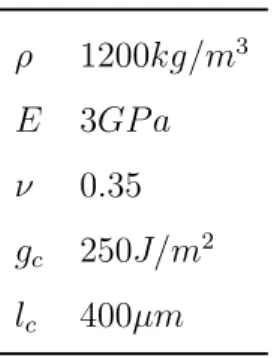
Table 2: Material properties considered in the phase-field simulation

media - a property to be discussed in the upcoming sections. We recall that for the hexagonal distribution, there’s only one characteristic length of the microstructure that is the distance between holes, denoted by d; while for the Penrose kite&dart paving, there are two characteristic lengths. As mentioned previously, the microstructure is modelled by the drilled holes inside a bulk material which mechanical properties are presented in Table 2. ρ is the material density, E and ν are respectively the Young Modulus

and Poisson ratio, lc is the internal length of the phase-field model and gc the

fracture toughness. In order to meticulously compare the microstructures,

the same hole radii rh = 750µm are taken, and the mean distances between

the holes is fixed to d = 3000µm corresponding to a volume fraction of

78% for the periodic microstructure and 75% for the quasi-periodic ones.

The generated microstructures are shown in Figure 3, and their respective geometrical aspects are displayed in Table 1. Two types of quasi-periodic microstructures are considered, both based on the kite&dart Penrose paving. Type 1 corresponds to the holes drilled at the nodes of the paving, while type 2 suggests drilling holes at the centroids of the kites and darts in the paving, leading thus to same-yet-different perfectly controlled microstructures each

217.5 mm 160 mm 65 mm 140 mm 70 mm 126 mm 50 mm bulk microstructure coarse-graining zone (a) (b)

Figure 4: Full (a) and close-up (b) diagrams of a typical finite element mesh of a TDCB specimen with the considered coarse-graining support mesh region (in light blue) allowing

the study of large scales lCGup to 10 times the mean distance between holes d.

one presenting specific quasi-periodic patterns. For the micro-mechanical simulations, the microstructure is put at the core of a Tapered Double Can-tilevered Beam (TDCB) fracture geometry to provide crack growth stability from the tapered profile of the specimen [31, 32]; the microstructure is sur-rounded by a homogeneous bulk material, the dimensions are put forth in Figure 4. Displacement boundary conditions are applied for the phase-field micro-mechanical simulation. In fact, the stability in crack growth provided by the TDCB specimen is believed to match the stability provided by the application of a surfing boundary condition [16]. In both cases, the crack evolves as it pleases inside the microstructure. In this study, the former

ourselves to the quasi-static evolution of cracks neglecting thus dynamics effects. The numerical discretization h = 200µm is thoughtfully adapted to the heterogeneities sizes and placements inside the domain and based

on [25], the internal parameter of the phase-field model lc is set to 400µm.

Both lengths are much smaller than the structure’s heterogeneities leading to mesh-independent crack initiation and propagation.

The influence of the microstructures on the crack propagation is prominent and put forth in Figure 3. For the periodic material, a simple linear crack path is obtained suggesting thus the presence of weak planes [30]. While for the quasi-periodic materials, each type proposes different-more tortuous paths suggesting more complexity of the damaging process. The influence of the microstructure is visibly reflected on both paths. A detailed crack path analysis is found in Section 3.4. After acquiring the simulation results,

a domain of interest Ω0 _{is considered for the study and then subdivided}

into finite constant-stress-constant-strain elements of size H = 1mm without loss of generality (Figure 4(b)).The considered coarse-graining function then sweeps over the mesh support constructing a database of mechanically and physically consistent fields at multiple larger scales to be analysed without any a priori on the model at each scale and by considering the physics happening

at the scale of heterogeneities. Ω0 _{is at the core of the microstructure which}

allows the use of large lCG and therefore large observation scales.

Exploiting the adapted coarse-graining method, one is able to investi-gate the microstructure at different transitional scales by building density, displacement, strain and stress fields at each scale.

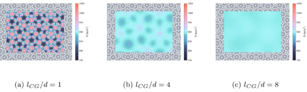
(a) lCG/d = 1 (b) lCG/d = 4 (c) lCG/d = 8

Figure 5: Effective density fields of type 1 quasi-periodic microstructure for three different scales.

3.2. Density

As established in the method, the density field R(x) is first computed. Effective density fields of the quasi-periodic type 1 microstructure at different

coarse-graining scales lCG are presented in Figure 5. Results actually show the

ability of the method to construct heterogeneous/homogeneous continuous density fields depending on the scale of interest without any a priori on the effective field’s homogeneity. To analyse the "homogenization" of the effective

density as the coarse-graining scale lCG is increased, we plot the evolution

of the mean and the coefficient of variation of R for the three considered microstructures (Figure 6 (a)). It’s considered that the homogeneity of a field is attained once its corresponding coefficient of variation COV drops below the ≤ 1% threshold. The arithmetic mean is calculated as the sum of the sampled values (whether at the nodes or the Gaussian points of the

coarse elements in Ω0_{) divided by the total number of samples (nodes and}

Gaussian points respectively). The standard deviation is found by taking the square root of the average of the squared differences of the values from their mean value. The coefficient of variation is defined as the ratio of the standard

0 2 4 6 8 10 l CG/d 600 700 800 900 1000 1100 1200 1300 R (kg/m 3) Periodic Quasi-Periodic - Type 1 Quasi-Periodic - Type 2 (a) 0 2 4 6 8 10 l CG/d 10-3 10-2 10-1 COV R Periodic Quasi-periodic - Type 1 Quasi-periodic - Type 2 1% (b)

Figure 6: Density conservation through mesoscales (a) and the evolution of the

correspond-ing coefficient of variation COVR defining the heterogeneity of the effective density

-evolution with lCG(b)

deviation to the arithmetic mean.

As the implemented coarse-graining method is based on the inviolable conservation laws - mass continuity between them -, it can be seen that the mean effective density in the studied domain is conserved through the scales and only the homogeneity of the field is altered. The heterogeneities of the effective density of the material are smeared-out much faster when considering

a periodic microstructure at lCG/d = 1, while the quasi-periodic

microstruc-tures require higher coarse-graining scales for the density heterogeneities to

smear-out at lCG/d = 4 (Figure 6 (b)).

3.3. Elastic Properties

Once the density fields are computed, manipulating the balance of mass at the fine and the coarser scale leads to the computation of the effective displacement fields that can be differentiated to determine the strain fields. The balance of linear momentum allows the evaluation of the effective stress

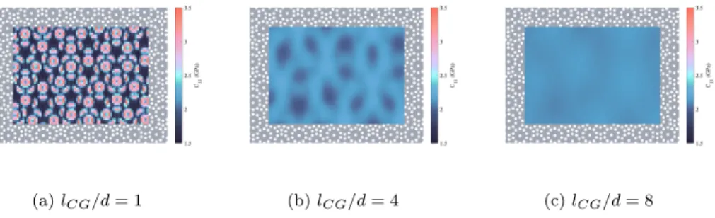
(a) lCG/d = 1 (b) lCG/d = 4 (c) lCG/d = 8

Figure 7: Fields of the C11 component of the effective elasticity tensor of type 1

quasi-periodic microstructure at three different scales.

fields. First, we aim to determine the behaviour of the material prior to dam-aging. For this purpose, we put the microstructure at the core of a rectangular specimen on which two tensile and one shear test simulations are conducted. From the microscopic mechanical fields, coarse-grained displacements, strains

and stresses can be evaluated for different lCG. Coarse-grained strain and

stress couples in Ω0 (obtained from the three tests) provide an evaluation

of the nine components Cij of the effective stiffness tensor C, representative

of the elastic behaviour, at each material point for the considered scales. It was observed that in the specimen coordinate system, the shear-extension coupling terms vanish; the reduced expression for the effective elasticity tensor written in (26) is thus adopted:

     S11 S22 S12      =      C11 C12 0 C21 C22 0 0 0 C66           E11 E22 2E12      (26)

Fields of the C11 component of the effective elasticity tensor of the

presented in Figure 7; the heterogeneity of C11 is shown to persist for large regularisation scales and thus the influence of the distribution of holes on the effective stiffness fields. From the computed effective elasticity tensors, both the anisotropy and homogeneity can be evaluated. As mentioned previously, the symmetry order of the studied periodic and quasi-periodic microstructures (6 and 5-fold symmetry respectively) are expected to lead to an equivalent isotropic response. From here, we aim to determine the scale from which the symmetry orders actually governs the elastic isotropy. To do so, the

two-dimensional elastic anisotropy index ar - defined in [33] - is analysed at

each material point for each observation scale. An explicit expression of ar as

a function of Cij and SCij can be written as follows:

ar = h1 4(C11+ C22+ 2C12)(SC11+ SC22+ 2SC12) − 1 i2 + 2h 1 16(C11+ C22− 2C12+ 4C66)(SC11+ SC22− 2SC12+ SC66) − 1 i2 !1₂ (27)

Where SCij represent the components of the compliance tensor SC defined as

SC = C

−1_{. a}

r takes the value of 0 in the case of perfect isotropy. Otherwise,

ar increases as the anisotropy strengthens. The main advantage of ar over

other anisotropy indices (Kube [34], Zener [35],...) is its direct applicability in 2D, for any symmetry type, and its direct evaluation from the elasticity

tensor. In this study, ar is computed from the evaluated elasticity tensors C

and SC at each material point of the domain for each coarse-graining scale

lCG. The distribution of these indices is shown in Figure 8. It’s observed

13 30 12 28 33 18 44 54 100 100 100 100 100 100 100 100 100 100 100 0.375 1 2 3 4 5 6 7 8 9 10 l CG/d 0 10 20 30 40 50 60 70 80 90 100

% isotropic material points

r= 0 + 1% + 3% + 5% (a) Periodic 13 11 13 24 19 26 37 17 29 48 14 59 35 85 14 100 100 100 100 100 100 100 100 0.375 1 2 3 4 5 6 7 8 9 10 l CG/d 0 10 20 30 40 50 60 70 80 90 100

% isotropic material points

r= 0 + 1% + 3% + 5% (b) Quasi-periodic type 1 11 12 7 19 18 14 28 21 23 37 22 48 43 8 79 20 100 100 100 100 100 100 100 100 0.375 1 2 3 4 5 6 7 8 9 10 l CG/d 0 10 20 30 40 50 60 70 80 90 100

% isotropic material points

r= 0 + 1%

+ 3% + 5%

(c) Quasi-periodic type 2

Figure 8: Material points distribution based on the elastic anisotropy index arcomputed

at different coarse-graining scales and for the considered microstructures.

(with an error lower than 1% ) once lCG is larger than the characteristic

length d of the microstructure. Although the material symmetry order of the quasi-periodic materials considered suggests elastic isotropic behaviour, it’s quite clear that this isotropy of the elasticity tensor cannot be reached at small scales but in fact, suggests a required scale of observation of at least 3 times the characteristic length d of the microstructure where the anisotropy indices of all the material points fall within 1% to 0 corresponding to the isotropy of the elasticity tensor in the whole domain.

Next, the homogeneity of the elastic moduli is put forth at different lCG. Only the observation scales at which the effective elasticity in the whole domain is isotropic (within 1% error) are considered in the study (Figure

8), i.e., lCG/d ≥ 1 for the periodic microstructure and lCG/d ≥ 3for the two

quasi-periodic microstructures. From the isotropic elasticity tensors fields, effective Young modulus (E) and Poisson ratio (ν) are computed for different

lCGon each element in the domain Ω0. Statistical analysis is conducted on the

evaluated effective elastic moduli to identify their possible "homogenisation" for each microstructure. The mean and standard deviation of the two material properties are plotted in Figures 9 and 10 as well as the evolution of the coefficient of variation of each property with the coarse-graining scale. The Poisson ratio converges and homogenises at considerably low length scales of observation. For the periodic microstructure, the effective Young modulus

is homogenised at considerably small observation scales (lCG/d = 1.5). The

average effective Young modulus for the different microstructures rapidly converges, contrary to its variation, especially for the quasi-periodic mi-crostructures where the effective Young modulus field requires larger length scales, at least 7 times the characteristic length d, to homogenise. Next, we proceed with the multi-scale damage analysis, starting with the influence of the observation scale on the crack path towards the effect on the strength and toughness fields as the crack advances inside the microstructures. 3.4. Crack Path

Displacement and stress fields from the phase-field simulations of fracture on the TDCB are upscaled, and coarse-grained displacements, strains and stresses with damage consideration are obtained. As the crack advances in

0 2 4 6 8 10 l CG/d 0 0.5 1 1.5 2 2.5 3

Equivalent Young (GPa)

Periodic Quasi-Periodic type 1 Quasi-Periodic type 2 (a) 0 2 4 6 8 10 l CG/d 10-3 10-2 10-1 COV E Periodic Quasi-Periodic type 1 Quasi-Periodic type 2 1% (b)

Figure 9: The effective Young modulus computed at different lCGfor the three

microstruc-tures (a) and the evolution of the corresponding coefficient of variation COVE - defining

the heterogeneity of the effective Young modulus - with lCG(b)

0 2 4 6 8 10 l CG/d 0.1 0.15 0.2 0.25 0.3 0.35 0.4 0.45 0.5

Equivalent Poisson ratio

Periodic Quasi-Periodic type 1 Quasi-Periodic type 2 (a) 0 2 4 6 8 10 l CG/d 10-3 10-2 10-1 COV Periodic Quasi-Periodic type 1 Quasi-Periodic type 2 1% (b)

Figure 10: The effective Poisson ratio computed at different lCGfor the three

microstruc-tures (a) and the evolution of the corresponding coefficient of variation COVν - defining

the microstructure, interactions between the crack and the structure of the material are observed, especially in the quasi-periodic microstructures. The crack can be expected to follow the path that would allow the maximum dis-sipation of energy. For type 1 quasi-periodic distribution, "resilient patterns" (red circles in Figure 11(b)) impose the deviation of the crack. For the type-2 quasi-periodic distribution, kinking of the crack is present, and due to the high amount of elastic energy stored in the specimen before kinking (red circles in Figure 11(c)), failure becomes unstable. The question arising here regards the ability to replace the complex crack path (at the microscopic scale) by an equivalent failure band (at larger scales of observations) represented by an effective straight crack path. To answer that question, the effective crack path at the coarse-grained scale is determined. Without loss of generality, we define the effective crack tip at time t as the local zone where the maximum stress occurs at this time t. By considering different criteria (Rankine, Maximum Volumetric Stress, ...) to evaluate the position of maximum stress, identical results were obtained; that is of course due to the stress singularity at the crack tip. The choice of the Rankine criterion naturally emerges for the description of brittle and quasi-brittle failure. From here, the effective "meso-scopic" crack tip position is defined as the local zone where the maximum Rankine stress is reached for each microscopic crack tip position. The length

scale introduced via the coarse-graining lCG method suggests softening of the

material (Figure 14 - more details about the stress-strain response is found in Section 3.5)- and an equivalency to a process zone is present suggesting that the critical stress before softening happens at a distance to the true crack tip (the crack tip determined from the micromechanical simulations). The

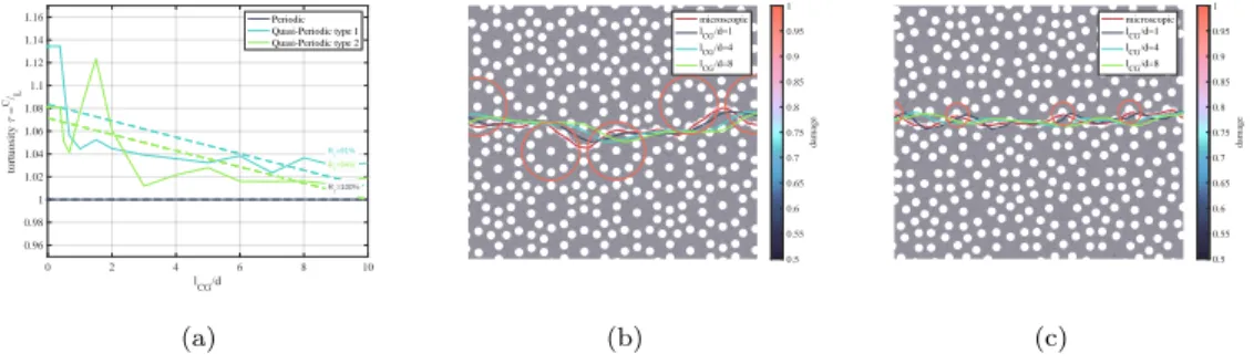
0 2 4 6 8 10 l CG/d 0.96 0.98 1 1.02 1.04 1.06 1.08 1.1 1.12 1.14 1.16 tortuosity = C/ L R =100% R =91% R =94% Periodic Quasi-Periodic type 1 Quasi-Periodic type 2 (a) 0.5 0.55 0.6 0.65 0.7 0.75 0.8 0.85 0.9 0.95 1 damage microscopic lCG/d=1 lCG/d=4 lCG/d=8 (b) 0.5 0.55 0.6 0.65 0.7 0.75 0.8 0.85 0.9 0.95 1 damage microscopic lCG/d=1 lCG/d=4 lCG/d=8 (c)

Figure 11: Mesoscopic crack paths for the type 1 (b) and type 2 (c) microstructures at

different lCGand the corresponding crack tortuosity evolution with lCG(a).

evolution of the crack paths and their corresponding tortuosity at different scales in the quasi-periodic microstructures are shown in Figure 11. Counter intuitively, one can observe prominent tortuosity of the crack path even at large scales. In fact, for the type 1 quasi-periodic microstructure, the crack

tortuosity only drops of less than 6% at lCG/d = 10 while the type 2 crack

path tortuosity drops around 9% from its microscopic value (Figure 11(a)). The conservation of the tortuosity across the considered scales drops the idea of the consideration of an effective straight failure band to replace complex crack paths. F F T analysis on the crack paths at different observation scales offers an insight on the amplitudes and wavelengths that contribute to the effective crack deflection. Later, the interaction between the wavelengths driving the crack deflection and the wavelengths driving the variations of the critical stresses and energy dissipation along the crack path are confronted. Figure 12 shows the F F T analysis results on the crack path inside the two quasi-periodic microstructures. As expected, small wavelengths λ/d ≤ 3 are smeared-out as the coarse-graining scale increases and more weight on the larger wavelengths is observed λ/d ≥ 10. The type 1 response shows decaying

0 1 2 3 4 5 6 7 8 9 10 11 12 13 14 15 16 17 18 19 20 21 22 23 24 25 /d 0 0.1 0.2 0.3 0.4 0.5 0.6 0.7 0.8 0.9 contribution to deflection microscopic l_CG/d=1 l_CG/d=2 lCG/d=3 l_CG/d=6 l_CG/d=9 (a) 0 1 2 3 4 5 6 7 8 9 10 11 12 13 14 15 16 17 18 19 20 21 22 23 24 25 /d 0 0.1 0.2 0.3 0.4 0.5 0.6 0.7 0.8 contribution to deflection microscopic l_CG/d=1 l_CG/d=2 lCG/d=3 l_CG/d=6 l_CG/d=9 (b)

Figure 12: FFT analysis on the mesoscopic crack path inside the quasi-periodic type 1 (a), and quasi-periodic type 2 (b) microstructures

amplitudes at wavelengths λ/d = 2 − 3 with a drop of about 62% (Figure 12(a)). The contribution of the wavelengths around λ/d = 5 corresponding to the distance between zones of "resilient patterns" (Figure 11(b)) is conserved through the scales and is responsible for 80% of the crack deflection. For the type 2 quasi-periodic microstructure, one clearly observe the absence of uniquely conserved high amplitude wavelengths across the scales (Figure 12(b)), except for λ/d = 2 − 3 that actually corresponds to the kinking spots. The crack path, in comparison with the type 1 -except for the kinking spots-does not conserve the same wavelengths suggesting a more easily smoothed crack path. Next, we focus on the influence of the microscopic heterogene-ity on the resistance and toughness fields at different coarse-graining scales, and we confront the wavelengths controlling the heterogeneities with the wavelengths present in the crack paths.

(a) lCG/d = 1 (b) lCG/d = 4 (c) lCG/d = 8

Figure 13: Upscaled vertical displacement Uy at different lCG. The discontinuity of the

displacement field is regularized by the coarse-graining function and dictated by its width

3.5. Fracture strength

Displacement and stress fields from the phase-field simulations of fracture on the TDCB specimens with the microstructures at their cores are upscaled, and coarse-grained displacements, strains and stresses with damage considera-tion are obtained. Figure 13 shows the vertical displacement field at different coarse-graining scales. The jump on the crack faces are smoothed as the observation scale increases and the sharpness of the crack at these scales is expected to be smeared out. A plot of the stress-strain relation computed at the coarse-grained scales of a TDCB test corresponds to a stress-strain response of a quasi-brittle behaviour (Figure 14). Here, the history of the hydrostatic stresses as a function of hydrostatic strains is plotted for different

points in Ω0.

As shown in Figure 14, the material undergoes a linear elastic trend followed by a non-linear region before reaching the critical stress where softening occurs. For small length scales, the increased width of the pack in the linear elastic region suggests heterogeneity of the modulus, to confirm the previous results regarding the homogenization of the elastic properties

strain stress Path strain stress Neighbourhood (a) lCG/d = 1 strain stress Path strain stress Neighbourhood (b) lCG/d = 4

Figure 14: Stress-strain behaviour of elements along the crack path and in a neighbourhood of the crack at two length scales lCG

of the materials. Non-uniqueness of the stress-strain response is observed when studying the response in a neighbourhood around the crack. The curve reaching the maximum stress corresponds to the response of the elements

along the crack path. As the distance to the crack path dcincreases, the

stress-strain response of the corresponding elements reach lower maximum stress states followed by some softening. When the elements are much further to the crack path, they remain undamaged and show typical linear elastic stress-strain response. For instance Figure 14 shows the stress-stress-strain response of a material in the neighbourhood of a crack at a specific abscissa in the domain,

at lCG/d = 1which corresponds to lCG= d = 3mm. As the coarse-graining

mesh size H is equal to 1mm, we find 6 different stress-strain responses of the elements corresponding to the discretization of the damageable zone. The

same trend is found at different coarse-graining scales lCG (Figure 14(a))

where a unique relation between the local stress and local strain states does not exist. Instead, as we move further from the crack path, and due to the regularizing nature of the coarse-graining, softening persists yet starts at lower critical stress levels leading thus to non-unique relations between the

stresses and strains. Non-locality of the fields is thus probable.

Moreover, when following the stress-strain response of the elements along the crack path, especially at low scales, and as the crack propagates through different patterns in the microstructure, the critical stress state reached before softening is found to differ from one position to another along the path. We define the maximum Rankine stress reached at each position of the crack

tip as the fracture strength or simply strength denoted σf, without abuse of

language. The evolution of the critical Rankine stress at different scales of observation is plotted in Figure 15 for the periodic (a), quasi-periodic type 1 (b) and quasi-periodic type 2 (c). The below figures thus show the significant influence of the local differences inside the microstructure - distribution of holes - on the fracture strength of the effective continuum. As the crack gets trapped inside the holes, much higher loading is required for the crack re-initiation, this phenomenon is mainly observed on the periodic geometry at the smallest scales, while for the quasi-periodic geometries, not only crack trapping influence the critical stress state reached, but also the crack deflection and deviation around the special "resilient patterns".

The strength fields at different coarse-graining scales lCG are studied and

both the average critical stress and its coefficient of variation over the crack

path for each length scale lCG are plotted in Figure 16. It’s clear that the

critical stress σf decreases when lCG increases. Moreover, a tendency stating

σf ∼ √_l1

CG is found. Similar expressions relating the tensile strength σf to

the characteristic length lc, E and gc are found in [25, 36, 37, 38] for gradient

and non-local damage models. Kindly refer to Section 3.6 for more details about this finding.

(a)

(b)

(c)

Figure 15: Fracture strength σf evolution along the crack path for the periodic (a),

In Figure 16, one observes higher strength for the periodic microstructure in comparison with the two quasi-periodic microstructures. A study on the evolution of the "homogeneity" of the strength is also conducted. Here, the coefficient of variation is evaluated by considering the squared differences of the values from the normalised values of a homogeneous response - allowing the study of the deviation of the strength surpassing the geometrical influences of the TDCB geometry and the loading conditions. Unlike the elasticity, the effective strength of the microstructures remains highly heterogeneous even

at large lCG. From Figure 16(b), it’s clear that the coefficient of variation

stabilizes nay slightly increases at large scales of observations independently of the microstructure. The coefficient of variation of the strength of type 1 and the type 2 microstructures stagnates at about 2% and 3% respectively.

The periodic’s COVσf converges to 0.6%. Counter-intuitively, the coefficient

of variation of the effective strength of the type 1 microstructure is lower than that of type 2 even though the path is more complex, but this may be caused by the presence of kinking in specific places leading to a huge increase of the loadings before the crack saps in comparison to the rest of domain where the crack path is smooth and straight.

Looking at Figure 15, it’s hard to quantify both the microstructural

effects and the influence of lCG on the fracture strength evolution in the

material. For this purpose, the fracture evolution is studied in the frequency domain, and F F T analysis allows to display the wavelengths and amplitudes to better depict the interactions of the microstructures and the coarse-graining impacting the strength. Figure 17 compares the wavelength spectrum of the

2 4 6 8 10 l CG/d 4 6 8 10 12 14 16 18 20 22 24 f (MPa) Periodic Quasi-Periodic type 1 Quasi-Periodic type 2 (a) 2 4 6 8 10 l CG/d 10-3 10-2 10-1 COV f Periodic Quasi-Periodic type 1 Quasi-Periodic type 2 1% (b)

Figure 16: Evolution of the mean fracture strength σf as a function of lCGfor the three

microstructures (a) and the evolution of the corresponding coefficient of variation COVσ_f

defining the heterogeneity of the effective strength field of the continuum (b)

amplitude is computed as the ratio of the amplitude of each wavelength to the RMS (root mean square) amplitude of the input signal. The periodic microstructure analysis shows a dominant peak occurring at a wavelength λ =

d corresponding to the length scale of the microstructure. The relatively low

(30%) drop of the contribution from the small scale to the largest considered

scale of λ = d suggests that the variation of the strength σf of the material is

controlled mainly by the distance d between the holes even on large observation scales for a periodic microstructure. This observation could explain the

stagnation of COVσf across the scales. As seen previously on the crack path

analysis, more weight is put on the larger wavelengths as the coarse-graining scales increase. The size of the holes does not present any influence on the strength variations. Regarding the type 1 quasi-periodic microstructure in Figure 17(b), one clearly observes the drop of the contributions of the small lengths scales and the rise of the contributions of the larger wavelengths as

the coarse-graining scales increase. The peaks on the wavelengths around

λ/d = 2 − 3 persist with increased influence as the scale of observation

enlarges. Comparing the F F T analysis of the crack path and the strength offers insights on the link between the wavelengths controlling the crack inside the microstructure and the effective strength. As the crack deflects mainly every λ/d = 5, it would have travelled two "resilient patterns" zones. This reflects the periodicity of the crack path that is twice the periodicity of the mechanical response. Once again, we can see that the main variation of the strength of the material is directly controlled by the distribution of holes. For the type 2 quasi-periodic microstructure (Figure 17(c)), even at the smallest scales, the heterogeneity of the strength comes from the long-range variations. At the smallest scale, 50% of the deviation comes from the larger wavelengths, which is due to the kinking that happen for the crack inside this microstructure at wide distances in the domain. Moreover, the small peak present at the small scale at λ/d = 1 corresponds to the crack travelling from one hole to another in a straight path between the kinking zones. The other small peak at λ/d = 2 − 3 (also met in type 1 microstructure) decays as the scale is increased. As the coarse-graining scale enlarges, the small wavelengths contributions are smeared out leading to the extreme rise of the influence of the large scales onto the strength variations.

3.6. Fracture toughness

The difference in the loading history of the material points inside the microstructure - whether distributed along their crack path or in the neigh-bourhood of a crack (Figure 14) - is directly related to the total amount of

0 1 2 3 4 5 6 7 8 9 10 11 12 13 14 15 16 17 18 19 20 21 22 23 24 25 / d 0 0.1 0.2 0.3 0.4 0.5 0.6 0.7 0.8 0.9 1 contribution to D f l_CG/d = 1 l_CG/d = 2 lCG/d = 3 l_CG/d = 6 l_CG/d = 9 (a) 0 1 2 3 4 5 6 7 8 9 10 11 12 13 14 15 16 17 18 / d 0 0.1 0.2 0.3 0.4 0.5 0.6 0.7 0.8 0.9 1 contribution to D f l_CG/d = 1 l_CG/d = 2 lCG/d = 3 l_CG/d = 6 l_CG/d = 9 (b) 0 1 2 3 4 5 6 7 8 9 10 11 12 13 14 15 16 17 18 19 20 / d 0 0.1 0.2 0.3 0.4 0.5 0.6 0.7 0.8 0.9 1 contribution to D f lCG/d = 1 l_CG/d = 2 l_CG/d = 3 lCG/d = 6 l_CG/d = 9 (c)

Figure 17: FFT analysis on the fracture strength σf for the periodic microstructure (a),

on the energy absorbed by the material points along the crack path. The

effective toughness Gd is defined as the energy to total failure evaluated as:

Gd =

Z tf

t0

S : ˙Edt (28)

allowing thus the measure of the energy dissipated per unit volume from the

start of the loading (t = t0) until the fracture of the specimen (t = tf). S

is the mesoscopic stress tensor and ˙E is the mesoscopic strain rate tensor.

The evolution of Gd at different scales of observation is plotted in figure 18

for the periodic (a), quasi-periodic type 1 (b) and quasi-periodic type 2 (c). The below figures thus show the significant influence of the local differences inside the microstructure -holes distribution- on the overall dissipated energy along the crack path of the obtained continuum. As the crack gets trapped inside the holes, much higher energy is required for the crack re-initiation, this phenomenon is mainly observed on the periodic geometry at the smallest scales, while for the quasi-periodic geometries, not only crack trapping influence the energy dissipation, but also the crack deflection and deviation around the special "resilient patterns".

A similar analysis to the one in Section 3.5 is conducted: a study of the

evolution of this toughness parameter Gd at different coarse-graining scales

followed by an F F T analysis to better understand the relationship between the microstructure and the effective toughness.

The average toughness Gd is inversely proportional to the coarse-graining

scale lCG (Figure 19(a)), and we find Gd ∼ _l1

CG. Indeed, coarse-graining

admits that the displacement, stress and strain fields on a material point actually depend on the state variables distribution in a neighbourhood of

(a)

(b)

(c)

Figure 18: Fracture toughness Gd evolution along the crack path for the periodic (a),

lCG. Here, we find Gd ∼ _l1

CG and σf ∼

1 √

lCG. As previously stated, similar

expressions relating the tensile strength σf to the characteristic length lc, gc

and E can be found in [25, 36, 37, 38]. From [25], the critical value of the tensile strength in uniaxial traction is given by:

σf = 9 16 r Egc 3lc (29)

This suggests the following: for a fixed toughness gc, the same relation

between σf and lCG holds between σf and lc: σf ∼ √1_l

c. Ultimately, for an

experimentally determined σf, the relationship Gd ∼ g_lcc stands. We recall

that the relations found in the literature hold only for uniaxial traction. We

mention that no consensus on the relation linking E, σf, lc and gc taking into

account the different loading conditions, and/or specimen geometries can be found in the literature. To emphasize, we recall that all the results presented in this paper are found without any a priori on the material behaviour at the coarse-grained scales.

A study on the evolution of the "homogeneity" of the effective toughness is conducted. In Figure 19, we plot the evolution of the effective fracture

toughness Gd as a function of lCG for the three microstructures (a) and the

evolution of the corresponding coefficient of variation COVGd defining the

heterogeneity of the effective toughness field (b).

As compared to the strength σf, one notices that the heterogeneity of

the toughness field Gd is higher than the one of the strength field at the

same scales. Yet no stability of the coefficient of variation of this quantity is observed at the large scales. As long as the crack path is straight, both the strength and the toughness evolve in the same manner at different

coarse-inversion of "homogeneity" of the toughness in comparison with the strength, i.e., when comparing the plots in both Figure (a) and Figure (b), the blue

and green curves corresponding to the coefficients of variation of σf and Gd

are inverted; COVσf is greater for the quasi-periodic type 2 microstructure

as compared to quasi-periodic type 1, while COVGd is smaller. In fact, the

crack might deflect to maximize its energy dissipation. This raises questions on the drift from LEF M where the notions of critical stress intensity factors and the critical energy release rate are somehow two faces of the same coin.

Again, F F T analysis transformed from the effective toughness deviation DGd

is presented in Figure 20.

For all three microstructures, small wavelengths λ/d ≤ 3 are smeared-out as the coarse-graining scale increases and more weight on the larger wavelengths is observed λ/d ≥ 10. In comparison with the strength responses, we can see that the larger wavelengths contributions to the heterogeneity

of the toughness fields significantly increase as lCG increases (a rise of more

than 100%) for all the microstructures). The peak on λ/d = 2 − 3 observed at the smallest scale for the type 1 microstructure (in both the strength and the toughness responses) is decreasing as the coarse-graining increases to give way to the larger wavelengths (see Figure 20). As compared to the F F T analysis of the fracture strength, the dominant peaks observed at smaller scales are no longer present through the observation scales and this suggests the following: as the regularization via coarse-graining increases, the

influence of the microstructure on Gdis smeared-out and the local phenomena

intervening in the energy dissipation process are smoothed, which can lead to an actual homogenisation of this parameter in comparison with the strength

2 4 6 8 10 l CG/d 10-2 10-1 100 Gd (kJ/mm 3) Periodic Quasi-Periodic type 1 Quasi-Periodic type 2 (a) 2 4 6 8 10 l CG/d 10-3 10-2 10-1 COV Gd Periodic Quasi-Periodic type 1 Quasi-Periodic type 2 (b)

Figure 19: Evolution of the effective fracture toughness Gd as a function of lCGfor the

three microstructures (a) and the evolution of the corresponding coefficient of variation

COVG_ddefining the heterogeneity of the effective fracture toughness field of the continuum

(b)

σf where the microstructural influence persists even for larger coarse-graining

scales.

4. Discussion and Concluding Remarks

This paper proposes a model-free coarse-graining method that does not require specific boundary conditions (as opposed to classical homogenisa-tion schemes) and is indeed applicable to non-periodic structures presenting high strain localisation. Aditionally, a model-free analysis of failure at the mesoscopic scale is performed. Phase-field simulation of failure on different microstructures was considered for the micromechanical simulations. The

obtained data are upscaled at different mesoscopic scales lCG via the

pro-posed coarse-graining technique that is solely based on the conservation laws. Density, displacement, stresses and strain fields at the mesoscopic scales are

0 1 2 3 4 5 6 7 8 9 10 11 12 13 14 15 16 17 18 19 20 21 22 23 24 25 / d 0 0.1 0.2 0.3 0.4 0.5 0.6 0.7 0.8 0.9 1 contribution to D Gd l_CG/d = 1 l_CG/d = 2 lCG/d = 3 l_CG/d = 6 l_CG/d = 9 (a) 0 1 2 3 4 5 6 7 8 9 10 11 12 13 14 15 16 17 18 / d 0 0.1 0.2 0.3 0.4 0.5 0.6 0.7 0.8 0.9 1 contribution to D Gd l_CG/d = 1 l_CG/d = 2 lCG/d = 3 l_CG/d = 6 l_CG/d = 9 (b) 0 1 2 3 4 5 6 7 8 9 10 11 12 13 14 15 16 17 18 19 20 / d 0 0.1 0.2 0.3 0.4 0.5 0.6 0.7 0.8 0.9 1 contribution to D Gd lCG/d = 1 l_CG/d = 2 l_CG/d = 3 lCG/d = 6 l_CG/d = 9 (c)

Figure 20: FFT analysis on the fracture toughness Gd for the periodic microstructure (a),

Quasi-brittle behaviour The coarse-graining method introduces a length scale which implies softening of the material - and thus an equiv-alency to a softening behaviour with a process zone, without any a priori on the behaviour at the larger scales. Plotting the stresses against the strains shows a typical response of quasi-brittle materials where a linear elastic region is followed by a non-linear region before softening. The notion of strength is thus notable.

Non-local effects Without any assumption on the material behaviour,

the absence of a unique behaviour law that links the local variables, i.e., local strains and local stresses, is illustrated. The stress-strain history of the elements at different distances to the crack path is different suggesting thus non-locality of the behaviour.

Once the behaviour at larger scales was established from the microscopic data, failure analysis was led on different heterogeneous materials, and for this purpose, three microstructures were considered: the periodic hexagonal distribution of holes and two types of kite&dart Penrose distribution of holes: at the nodal positions (type 1) and on the centroids of the kites and darts (type 2). A study on the effective material properties was led followed by a failure analysis to further understand interactions between the cracks, the scales and the microstructures.

Density The equivalent densities at different coarse-graining scales are

conserved - an expected results since the essence of the coarse-graining method is the conservation principles. A homogeneous density field (COV < 1%) is

obtained at lCG/d = 1 for the periodic and lCG/d = 4 for the quasi-periodic

Elastic properties From the micromechanical simulations before failure, coarse-grained elastic stresses and strains allowed the computation of elasticity fields. Although the anisotropy of a microstructure is depicted by its symmetry order, the proposed scheme shows that a relatively large observation scale is

needed for the symmetry order to reveal its influence. From the scale lCG/d =

1, isotropy converges for the periodic microstructure while the isotropy of

the quasi-periodic structure requires lCG/d = 3. The heterogeneities found

at the microscopic scale influence the equivalent elastic properties at the mesoscopic scale. We show that in order to consider a homogeneous isotropic

elastic equivalent medium, the required lCG exceeds the values considered

in the literature and in fact is much larger when considering non-periodic microstructures with long-range heterogeneities. For the periodic distribution,

an equivalent isotropic homogeneous elastic medium is found starting lCG/d =

1.5, while for both quasi-periodic distributions, an lCG/d = 7 is required to

obtain an equivalent elastic homogeneous medium.

Crack path Phase-field simulations on the considered microstructures

showed highly complex crack networks especially for the quasi-periodic mi-crostructures. The effective crack path was analysed at different observation scales. We define the crack tip at each time step as the position at which the equivalent Rankine stress is maximum. The evolution of the crack paths shows prominent tortuosity across the observation scales. F F T analysis on the crack paths offered insight on the amplitudes and wavelengths that contribute to the effective crack paths. For the type 1 quasi-periodic microstructure, peaks at similar wavelengths for different coarse-graining scales persist suggesting thus that the microstructural distribution of holes underlines the

conserva-tion of the tortuosity and prohibits the consideraconserva-tion of a smooth effective failure band. For the type 2 microstructure, one clearly observes the absence of uniquely conserved high amplitude wavelengths across the scales which suggests a more readily smoothed crack path between the kinking spots.

Fracture strength The notion of strength emerging from the obtained

coarse-grained stress-strain response was analysed. We define the fracture strength as the critical equivalent Rankine stress state reached at each effective crack tip position. The effective fracture strength is found to vary from one position of the crack tip to another along the crack path. This is explained by different phenomena including the trapping, re-nucleation, and deflection of the cracks after advancing inside the microstructure. This property is found to be the hardest to smear-out; in fact, the influence of the microstructure persists in all three microstructures even for relatively large coarse-graining scales. The stagnation of the coefficient of variation of the strength for the considered microstructures suggests the inability of the consideration of a homogeneous strength field for an effective medium that takes into account the heterogeneities at the smaller scales and that has a dominant role in stress concentration, crack initiation and general propagation. To better understand the microstructure’s influence coupled with the scales, F F T of the crack paths and the fracture strengths are confronted. Even at large coarse-graining scales, i.e., where smoothing of local phenomena is expected, the strength remains highly influenced by the relatively small scales of the microstructures and large wavelengths do not have a significant influence on this quantity.

This, with the evolution of the coefficient of variation of σf leads to believe

the fracture strength field of locally heterogeneous material.

Fracture Toughness We also proposed a definition of the fracture

toughness. Following the evolution of the coefficient of variation for the different microstructures, coarse-graining shows good ability to smear-out the microstructural effects on the equivalent toughness with no stagnation of the coefficient of variation at the large scales. F F T analysis of the fracture toughness evolution in the domain shows the large wavelengths contribu-tions suggesting more easily smoothed parameter in comparison with the fracture strength, whereas the small wavelength amplitudes related to the microstructures are smeared-out.

This leads us to believe that considering a homogeneous model for sim-ulating quasi-brittle failure in highly heterogeneous materials requires the consideration of extremely large scales to always be on the safe side when considering equivalent isotropic homogeneous properties. We also show the inevitability of the consideration of a non-homogeneous material in which the influence of substructures is preserved at the mesoscopic scales.

Open issues and extensions Within the proposed framework, we are

able to perform a micro-meso analysis of quasi-brittle failure on periodic and quasi-periodic materials. The examples presented herein are limited to quasi-static crack propagation with imposed displacement. The absence of branching and multi cracks limited the analysis to a single crack propagation. The consideration of the phase-field model at the microscopic scale to build the ground for the multi-scale analysis presented some limitations, especially regarding the model parameter and the calculation times. Yet, once the micromechanical data are obtained, the proposed coarse-graining method can