Coverage problems in mobile sensing

Coverage Problems in Mobile Sensing

by

Ajay A. Deshpande

B.Tech., M.Tech., Mechanical Engineering

Indian Institute of Technology Bombay, 2001

S.M., Mechanical Engineering

Massachusetts Institute of Technology, 2006

S.M., Electrical Engineering and Computer Science

Massachusetts Institute of Technology, 2006

Submitted to the Department of Mechanical Engineerin

in partial fulfillment of the requirements for the degree

Doctor of Philosophy

_{DEC 0 7 2008}

at the

_LIBRARIES

MASSACHUSETTS INSTITUTE OF

TECHNOLOGY-September 2008

@

Massachusetts Institute of Technology 2008. All rights reserved.

Author ...

Department of Mechanical Engineering

Sugust 28, 2008

Certified by

...

...

Sanjay E. Sarma

Associate Professor of Mechanical Engineering

Thesis Supervisor

Certified by

...

...

Daniela Rus

Professor of Electrical Engineering and Co puter Science

~E4is

Supervisor

Accepted by

...

Lallit Anand

Chairman, Department Committee on Graduate Students

Coverage Problems in Mobile Sensing

by

Ajay A. Deshpande

Submitted to the Department of Mechanical Engineering on August 28, 2008, in partial fulfillment of the

requirements for the degree of Doctor of Philosophy

Abstract

Sensor-networks can today measure physical phenomena at spatial and temporal scales that were not achievable earlier, and have shown promise in monitoring the environment, structures, agricultural fields and so on. A key challenge in sensor-networks is the coordination of four actions across the network: measurement (sens-ing), communication, motion and computation. The term coverage is applied to the central question of how well a sensor-network senses some phenomenon to make infer-ences. More formally, a coverage problem involves finding an arrangement of sensors that optimizes a coverage metric.

In this thesis we examine coverage in the context of three sensing modalities. The literature on the topic has thus far focused largely on coverage problems with the first modality: static event-detection sensors, which detect purely binary events in their immediate vicinity based on thresholds. However, coverage problems for sensors which measure physical quantities like temperature, pressure, chemical concentrations, light intensity and so on in a network configuration have received limited attention in the literature. We refer to this second modality of sensors as estimation sensors; local estimates from such sensors can be used to reconstruct a field. Third, there has been recent interest in deploying sensors on mobile platforms. Mobility has the effect of increasing the effectiveness of sensing actions. We further classify sensor mobility into incidental and intentional motion. Incidentally mobile sensors move passively under the influence of the environment, for instance, a floating sensor drifting in the sea. We define intentional mobility as the ability to control the location and trajectory of the sensor, for example by mounting it on a mobile robot.

We build our analysis on a series of cases. We first analyze coverage and connec-tivity of a network of floating sensors in rivers using simulations and experimental data, and give guidelines for sensor-network design. Second, we examine intentional mobility and detection sensors. We examine the problem of covering indoor and out-door pathways with reconfigurable camera sensor-networks. We propose and validate an empirical model for detection behavior of cameras. We propose a distributed al-gorithm for reconfiguring locations of cameras to maximize detection performance. Finally, we examine more general strategies for the placement of estimation sensors

and ask when and where to take samples in order to estimate an unknown spatio-temporal field with tolerable estimation errors. We discuss various classes of error-tolerant sensor arrangements for trigonometric polynomial fields.

Thesis Supervisor: Sanjay E. Sarma

Title: Associate Professor of Mechanical Engineering Thesis Supervisor: Daniela Rus

Acknowledgments

First of all, I would like to thank my advisors, Sanjay Sarma and Daniela Rus, without whose support and invaluable guidance this work would not have been possible.

Words are not enough to express my gratitude towards Sanjay. I have learned so much from him through his unique research-style. He gave me complete freedom in terms of the classes that I took and the problems I chose to work on and I value that a lot. I am simply held in awe by his in-depth understanding of a wide range of areas, his ability to ask right questions, his vision and bold approach to research. Besides research, he has given me invaluable advice on various other aspects of life for which I will be forever indebted to him. His energy and enthusiasm are highly contagious. I truly thank him for the TA opportunities he gave me. Sanjay, thanks a lot for everything!

I am truly grateful to Daniela for having given me an opportunity to work in her group. I have learned a great deal from her about research over the last few years. I am amazed by her energy and her ability to successfully run such a large research group. I thank her for providing work-space in Stata Center. I thank her for the opportunity she provided me to collaborate with our collaborators at the University of Southern California. I also thank her for generously funding my conference trips.

I am grateful to Devavrat Shah for being an excellent mentor for the last few years at MIT. I truly appreciate the constructive criticism he gave me on my research. I also thank him for detailed comments on my thesis.

I would like to thank Dr. David Brock for several useful suggestions during the committee meetings and comments on the thesis.

Work discussed in Chapter 4 was done in collaboration with Sameera Poduri and Gaurav Sukhatme at the University of Southern California. I am thankful to them for this great collaboration. I had several fruitful discussions with Sameera during our meetings and over phone. I am thankful to Gaurav for his useful comments on work in the second part of this thesis.

I truly acknowledge pointers provided by Prof. Vivek Goyal on related work in 5

frame theory.

I thank Prof. Harold Hemond for useful discussion on river work. I would also like to thank David Holtschlag of the USGS for generously providing me with their experimental data used in Chapter 3 of this thesis.

I would like to thank all the current and former members of Sanjay's research group, Rahul Bhattacharyya, Isaac Ehrenberg, Christian Floerkemeier, Patrick Hacker, Stephen Ho, Kashif Khan, Taejung Kim, Sriram Krishnan, Sumeet Kumar, Kirti Mansukhani, Seung-Kil Son and Marty Vona for creating wonderful atmosphere at the workplace. I would like to thank Sriram for being an excellent mentor and a great office mate over the years. I collaborated with Taejung Kim on art-gallery work and learned a lot from him about paper writing. I would like to thank Stephen Ho for proof-reading an early draft of this thesis and providing several useful sugges-tions. I thank him for several fruitful discussions we have had over the last year. I would like to thank Christian Floerkemeier for several discussions we have had over lunch. I would especially like to thank Christian and Stephen for taking time out to patiently listen to my defense practice presentation and providing so many useful suggestions. I would also like to thank Edmund Schuster for several useful discussions on applications of my work, and his kind and encouraging words.

I would also like to thank the members of Daniela's research group (Distributed Robotics Laboratory), especially Mac Schwager and Marty Vona, for so many useful discussions.

I would like to thank David Rodriguera and Rachel Russell of the Laboratory for Manufacturing and Productivity along with Leslie Regan and Joan Kravit at the

Graduate Office of Mechanical Engineering for the incredible support they provided on the administrative front. Because of them I never had to bother about any

ad-ministrative issues.

I was fortunate enough to have a great set of friends at MIT. I would like to thank Sreekar Bhaviripudi, Shashibhushan Borade, Amit Deshpande, Rohit Karnik, Dhanushkodi Mariappan, Ashish Shah, Vijay Shilpiekandula, Amit Surana, Kripa Varanasi and Murtaza Zafer. I have spent real quality time with these guys and have

learned a lot from each one. I will forever cherish the fun-times we have had together. I have spent countless hours with both the Amits, Vijay, Dhanush and Kripa chatting over afternoon coffee, lunches and dinners. These guys are like my brothers. I would also like to thank my friends in other parts of the world including my school friends and my IIT friends.

I would like to thank all my relatives and friends back in India for their support and love. They have always made my every trip to India a memorable one. I would like to thank Sunita (my brother's wife) for her support and encouragement. I thank Amma-Appa (my in-laws) for treating me like their own son. I thank Prahladh for being a big brother. He has left indelible impressions in my life through his thoughts and actions, and continues to inspire me. If not for him, I would have never met Pavithra, my wife and his sister! Finally I would like to thank my dearest wife Pavithra, my brother Nitin, Aai (Alka Deshpande) and Baba (Ashok Deshpande) for their constant love and endless encouragement. To them I dedicate this thesis. Pavithra, the sweetest dream unfolded before my eyes, brings the spark in my life and is the biggest source of my strength. Nitin has always been my true friend, philosopher and role model in life. Aai-Baba have made countless sacrifices and molded me into what I am today. I attribute my success so far to my parents and my brother.

To Aai, Baba, Nitin and

Contents

1 Introduction 21

1.1 Problems addressed in this Thesis . ... . 22

1.2 Summary of our Contributions ... ... 24

1.3 Structure of this Thesis ... 26

2 Literature Review 29 2.1 Sensor Networks ... ... 29

2.1.1 What is a sensor network? . . . . 30

2.1.2 Applications ... . ... 31

2.1.3 Differences with Traditional Network Design . ... 32

2.2 Coverage Problems in Sensor Networks . ... 33

2.2.1 Sensors Classification . ... .... 34

2.2.2 Mobility classification ... .... 35

2.3 Detection Sensors with Disc Coverage Model Floating in Rivers . . . 37

2.3.1 Motivation for the river application . ... 37

2.3.2 Coverage and connectivity with respect to a disc model . . . . 38

2.4 Intentionally-mobile Detection Sensors with Utility-based Coverage 39 2.4.1 Coverage Problem Formulation . ... 40

2.4.2 Distributed Control and Coordination Algorithm ... . 41

I

Detection Sensors

3 Floating Event-Detection Sensors in Rivers 3.1 Natural mobility of sensors in rivers ...

3.1.1 Ideal-channel rivers . . . . . . . . . . . ..

3.1.2 Natural rivers ... . ....

3.2 Coverage problem... ....

3.3 Coverage analysis for an ideal river mobility . . . . 3.3.1 Initial deployment . . . . . . . . . . . .. 3.3.2 An approximation: constant longitudinal velocity walk 3.4 Connectivity problem . . . . . . . ..

3.4.1 Connectivity challenges . . . . 3.5 Connectivity analysis for an ideal river mobility . . . . 3.6 Experimental Data and Simulation results . . . . 3.6.1 Experimental Data source . . . ..

3.6.2 Simulation settings ... ...

3.6.3 Coverage results ... ...

3.6.4 Connectivity results ... 4 Reconfigurable Camera Sensor Networks

4.1 Coverage Problem Formulation . . . .

4.1.1 Partial derivative of the overall utility function . . . . . 4.2 Distributed coverage control . . . ..

4.2.1 Control Law for each sensor . . . . 4.2.2 Distributed Coverage Algorithm . . . .

4.2.3 Convergence . . . . . . . . . . . ..

4.3 Deployment of Cyclops camera networks . . . . 4.3.1 Sensing Performance Function . . . .. 4.3.2 Coverage Algorithm for 1D loop . . . . 4.4 Simulation Results ... 4.4.1 Simulation Environment . . . . 47 . . . 47 . . . 49 . . . 51 .. . 52 . . . 54 . . . 55 . . . 56 . . . 59 . . . 61 . . . 61 . . . 63 . . . 64 .. . 69 .. . 69 .. . 73 83 84 85 86 86 87 88 88 89 91 94 94

45

4.4.2 Global knowledge of sensor performance function 4.4.3 Occlusions ...

4.4.4 Online estimation of sensor performance function 4.4.5 Cyclops Experiments and Results . . . . 4.4.6 Indoor experiments ...

4.4.7 Outdoor experiments . . . .

4.4.8 Dynamic Environments . . . .

II Estimation Sensors

5 Frame Theory and Non-uniform Sampling 5.1 B asis . . . . 5.2 Fram es . . . .

5.2.1 Frame Fundamentals ... 5.2.2 Tight Frames ... 5.2.3 Frame Algorithms ...

5.3 Pseudo-inverse and Linear Estimation .... 5.4 Non-Uniform Sampling ... 107 . . . . 108 . . . . 109 . . . . 109 . . . . . . 112 . . . . . 115 . . . . 116 . . . . 118

6 Error Tolerant Arrangements of Estimation Sensors 6.1 Sensor Arrangement Problem . . . . 6.1.1 Field M odel . .. . .. . . .. . . . .. . .. . .. .. . 6.1.2 Measurement Model and Matrix Representations . . . . . 6.1.3 Linear Reconstruction . . . . 6.1.4 Sensor Arrangement Problem . . . . 6.1.5 Relevance to non-uniform sampling and frame theory . . . 6.2 Our Approach: Error Tolerant Arrangement Classes (ETAC's) . . 6.3 ETAC's for Trigonometric Polynomials . . . . 6.3.1 Trigonometric polynomials . . . . 6.4 Regular Sensor Arrangements . . . . 6.4.1 Regular arrangement with the same period along each axis 94 97 98 100 .. 100 . . 101 . . 103

105

6.4.2 Regular sensor arrangement with different sampling periods

along each direction ... .. . . 140

6.4.3 Line-regular sensor arrangement . ... 141

6.5 A-dense Sensor Arrangement ... ... . . 144

6.6 Incrementally Constructed Sensor Arrangements . ... 146

6.7 Random Sensor Arrangements ... ... ... 151

6.7.1 Sensor arrangement with one randomly placed sample per grid cell ... ... ... 154

6.7.2 Uniformly random sensor arrangement . ... 163

6.8 On the i.i.d. noise assumption ... ... 165

7 On Mobility of Point Estimation Sensors 169 7.1 A few motion-related probleims overlay-ed on ETACs . ... 170

7.1.1 A-dense sensor arrangements . ... 170

7.1.2 Random sensor arrangements . ... 173

8 Conclusions and Future Work 175 8.1 Conclusions ... ... 175

List of Figures

3-1 Ideal channel coordinate system and profile. The z-axis and y-axis indicate the vertical and transverse directions respectively. The x-axis is not shown in the figure. It comes out of the page and indicates the

longitudinal direction of the flow. . ... . . . . . 49

3-2 Area swept by the coverage-discs of 9 nodes that move according to the mobility model in an ideal-channel river with the simulation parameters

described above ... 54

3-3 Connectivity versus time for 50 nodes deployed uniformly randomly along the transverse cross-section in an ideal-channel river. The

com-munication range of each nodes is 75m. ... . . . . 62

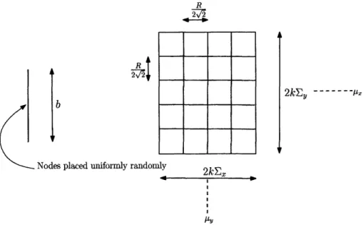
3-4 Grid arrangement useful in the analysis of connectivity ... 63

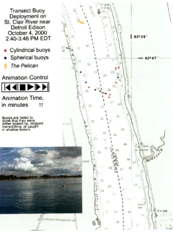
3-5 St. Clair River near Detroit Edison. The snap-shot of the animation

is obtained from the USGS website ... 65

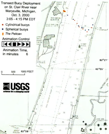
3-6 St. Clair River near Marysville. The snap-shot of the animation is

obtained from the USGS website. ... 66

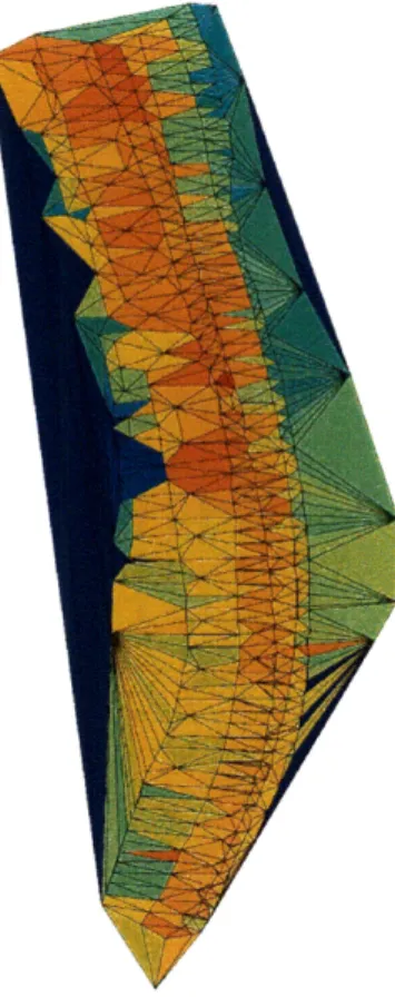
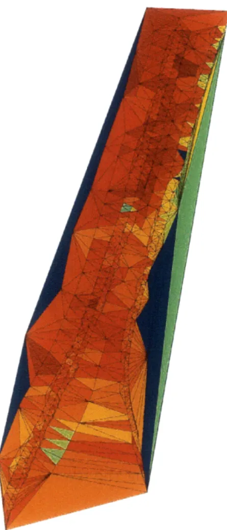
3-7 The velocity field using the mesh model for Detroit Edison site. . .. 67 3-8 The velocity field using the mesh model for Marysville site ... 68

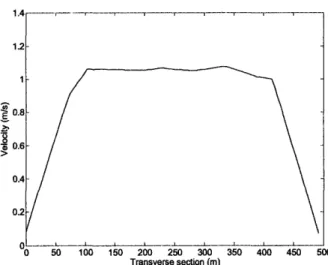
3-9 Edison velocity profile ... 68

3-10 Marysville velocity profile ... ... 69

3-11 Coverage results for the natural mobility in the ideal-channel river for

sensors with coverage radius = 20m . ... 70

3-12 Coverage results for the mesh model of St. Clair River at Edison for

3-13 Coverage results for the mesh model of St. Clair River at Marysville

for sensors with coverage radius = 20m ... 72

3-14 Connectivity vs. Time for nodes with communication range 75m in

the ideal-channel river in the central zone . ... 74

3-15 Connectivity vs. Time for nodes with communication range 75m in St. Clair River near Detroit Edison in the central zone . ... . 75 3-16 Connectivity vs. Time for nodes with communication range 75m in St.

Clair River near Marysville in the central zone . ... 76

3-17 Connectivity vs. Time for nodes with comnmunication range 75m in

the ideal river in the side zone ... ... 77

3-18 Connectivity vs. Time for nodes with communication range 75m in St. Clair River near Detroit Edison in one of the side zones ... . . 78 3-19 Connectivity vs. Time for nodes with communication range 75m in St.

Clair River near Marysville in one of the side zones . ... 79

3-20 Connectivity vs. Time for nodes with communication range 75m in St. Clair River near Detroit Edison in the other side zone . . . . ... 80 3-21 Connectivity vs. Time for nodes with communication range 75m in St.

Clair River near Marysville in the other side zone . ... 81

4-1 Cyclops camera, with an attached Mica2 Mote . ... 88

4-2 Perspective projection model ... ... ... . 89

4-3 Illustration of pixels on target not detected. (a) background image (b) original image and (c) foreground image. In the foreground image, some of the pixels in the target board are black. These are the pixels

that are similar to the background and are therefore not detected by

4-4 Validation of the proposed model for pixels detected vs. distance for three different environments. 1(a) is a well-lit corridor and close to an ideal environment. 2(a) is an outdoor pathway with shadows of trees and buildings. 3(a) is inside a lab where the lighting conditions are not uniform. The solid blue line is the number of pixels detected from experiments and the red dashed line is the minimum least squares fit

using the model in Equation 4.6 . . ... .. . . 92

4-5 Performance of the distributed control law for three types of parameter functions on a 1D loop which is a 250 feet long smooth curve. 1(a), 2(a) and 3(a) show the parameter values constant, sine and step. 1(b), 2(b) and 3(b) show the corresponding final positions of sensors (red circles) superimposed on the k function. The crosses show the dominance region boundaries between sensors. 1(c), 2(c) and 3(c) show the vari-ation in the net coverage utility. The utility increases monotonically

with each iteration ... ... 95

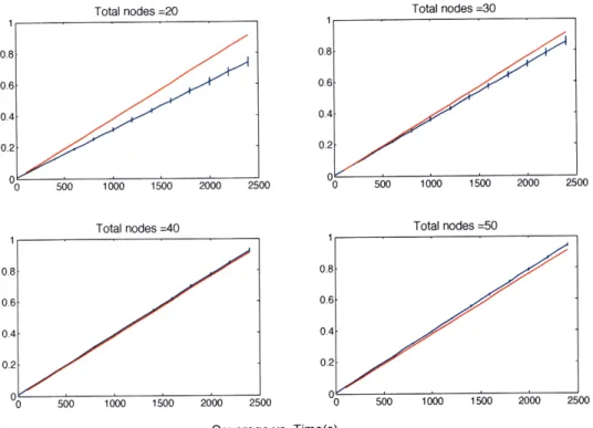
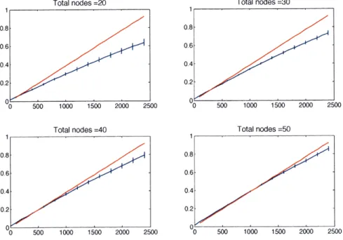
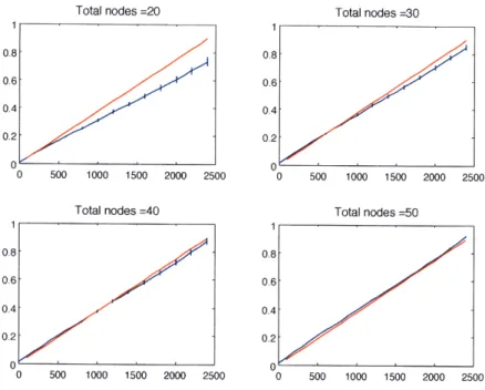
4-6 Variation in coverage utility and convergence time for different network

sizes averaged over 50 iterations ... 96

4-7 Performance of the distributed control law in the presence of occlusions

- (1) obstacles and (2) sharp corners. . ... . . 96

4-8 Performance of the distributed control law with partial knowledge of

ki(x) and k2(X) ... ... 99

4-9 Cyclops setup ... ... 99

4-10 Performance of the distributed control law in an indoor rectangular

corridor ... ... 101

4-11 Performance of the distributed control law in an outdoor environment. 102 6-1 (a) Regular sampling with the same period along both axes (b) Regular

sampling with different periods along each axis (c) Line-regular sampling 140 6-2 M = 3, a02 = 1; samples are uniformly placed at points of a regular

6-3 For the arrangement shown in Figure 6-2, Err(X) is shown as a function of (x, y) where (x, y) is added to the already existing arrangement of samples. There are many local optima. The estimation error is reduced the most when the sample is placed at the missing sample site. .... 148 6-4 Voronoi diagram for a set of points randomly placed in 2D domain.

This Voronoi diagram conforms with the toroidal nature of the

sam-pling domain .. ... ... ... 149

6-5 64 sample sites are randomly chosen. 10 additional sample points ob-tained using the brute force search method and our heuristic are shown

along with the initial randomly chosen sites. . ... 151

6-6 For the arrangement shown in Figure 6-5, Err(X) is shown as a function of (x, y) where (x, y) is added to the already existing sensor arrange-ment. The resolution between consecutive points is 0.01. There are

many local optima. ... 152

6-7 Comparison of the estimation error values for three different schemes of incremental sampling: (1) the brute force search method for global minima at each step carried at resolution of 0.01 (2) our heuristic based on Voronoi diagrams to choose initial point for optimum search at each step (3) random selection of an initial point for optimum search at each

List of Tables

1.1 Our categorization of sensors and mobility types and the coverage

prob-lems addressed in this thesis ... 24

2.1 Our categorization of sensors and mobility types and the coverage

Chapter 1

Introduction

Wireless sensor networks have revolutionized the way we can collect information about the physical world. Advances in three key technologies, integrated circuits, wireless communications, and micro and nano-mechanical systems in the last two decades lead to the advent of cheap, low-power and compact wireless sensors. These sensors have shown great promise in monitoring urban and natural environments, structures, agricultural fields, industries, and so on by providing data at spatial and temporal scales that were not achievable before. For example, in structural monitoring appli-cations, wireless sensors regularly monitor the health of structures such as buildings and bridges, and can warn of impending failures. As another example, sensors fixed at traffic signals combined with sensors on automobiles can provide real-time update on traffic conditions in urban environments. In each application, sensors provide real-time mapping of some aspects of the physical world.

Each sensor in a sensor-network embodies three abilities: sensing, communication and computation. If a sensor is mounted on a mobile agent such as a robot, an animal or a float in water, it has yet a yet another ability, mobility. In the cost, size and power-regime of sensors that we consider suitable for sensor-networks applications, a sensor is heavily constrained in each of its abilities. Sensors have limited battery-life, memory, computational capacity, and sensing resolution. They are also prone to failures. Power and adverse mobility patterns heavily limit communication ability. The main challenge in a sensor-network is the coordination of sensors' limited abilities

across the network for the desired application. However, despite these limitations, sensor-networks have demonstrated success in quite a few applications. Since its emergence towards the end of the last century, sensor-networks has been an active area of research and still in its early stage.

A central question in sensor-networks is how well sensors can sense and map some physical phenomenon. For example, in structural monitoring applications, we may ask how many sensors we may need and where we mount them on a structure or how reliable are the overall inferences about the sensors' measurements. It seems that one configuration might be better over the other configuration of the sensors in the sense of sensing quality. The term coverage problems applies to the class of problems that implicitly tries to address these questions. More formally, a coverage problem involves formulating an overall coverage metric based on an individual sensor's behavior and optimizing it over different configurations. This thesis addresses coverage problems in sensor networks with special emphasis on mobile sensing.

1.1

Problems addressed in this Thesis

The overall coverage metric depends on an individual sensor's sensing behavior, which in turn depends on the kind of sensors. The literature on coverage problems thus far has focused on static sensors that detect purely binary events in their immediate vicinity based on thresholds. It is possible to associate a spatial sensing-performance

fanction with each sensor. For example, some sensors can detect the presence of an

event only within a certain range. The sensing-performance function in this case can be a step function that is 1 over the circular disc of radius equal to the range and 0 ev-erywhere else. This model is known as the disc model of coverage in the literature. In yet another example, some sensors can have an explicit sensing performance-function in which performance decreases as a function of distance. We call this type of sensors

event-detection sensors. Apart from event-detection sensors, there is another type

of sensors in which sensors measure physical quantities like temperature, pressure, chemical concentrations, light intensity and so on in a network configuration. We

refer to this type of sensors as estimation sensors. In estimation applications, local estimates are used to reconstruct the spatio-temporal field of the unknown physical quantity. Coverage problems for such sensors have received limited attention in the literature. In this thesis, we address coverage problems for both event-detection and estimation sensors.

Recently, there has been great interest in deploying sensors on mobile platforms such as robots, floats in water, animals, and cars. Mobility adds another degree of freedom in coverage problems. It has the effect of increasing the effectiveness of sensing actions and can significantly alter the definition of the coverage metric. For example, the coverage of a mobile sensor with the disc nmodel is the area covered by the sweeping of the disc. We classify sensor mobility into incidental and intentional motion. Incidentally mobile sensors move passively under the influence of the en-vironment, for instance, sensors attached to animals or a floating sensor drifting in the sea. We refer to a sub-class of incidental motion where sensors move under the influence of natural forces as natural mobility. We define intentional mobility as the intentional control of the location and trajectory of the sensor. An example is a sensor mounted on a mobile robot. This thesis addresses the three categories of coverage problems at the intersection of both mobility models, incidental and intentional, and both sensor types, detection and estimation. In summary, the problems we address are:

1. Naturally mobile event-detection sensors in rivers: We address the cov-erage of floating sensors moving passively in rivers. We consider event-detection sensors with the disc model. The disc model is also used to miodel comnluni-cation between two nodes. Two nodes can communicate with each other if the distance between them is less than the communication range. We analyze the

connectivity of the moving network.

2. Reconfigurable camera-networks: We examine the problem of covering in-door and outin-door pathways using a reconfigurable camera-network where cam-eras are intentionally mobile. We also address the problem of modeling the

detection behavior of an individual camera.

3. Sensor arrangement problem: We introduce the sensor arrangement prob-lem as a kind of coverage probprob-lem for the estimation sensors that provide local sample values of a field of some physical quantity. The samples can be used to reconstruct the unknown field. Using the sampling theory and estimation theory, we formulate the coverage metric as the error in the field reconstruction. The error is a function of the geometric arrangement of the sensors. The sensor arrangement problem addresses the question of when and where to take samples in order to estimate an unknown spatio-temporal field with tolerable estimation errors.

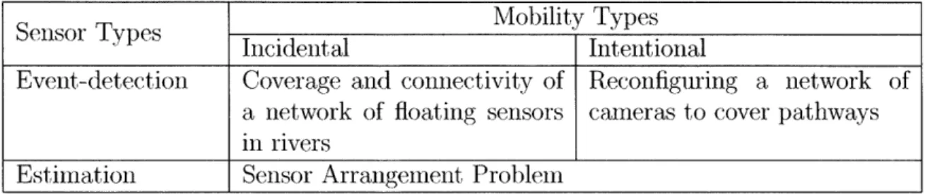
The table below shows our categorization of the sensors and mobility types, and the combinations we address.

Table 1.1: Our categorization of sensors and mobility types and the coverage problems addressed in this thesis

Mobility Types

Incidental Intentional

Event-detection Coverage and connectivity of Reconfiguring a network of

a network of floating sensors cameras to cover pathways in rivers

Estimation Sensor Arrangement Problem

1.2

Summary of our Contributions

A summary of our contributions for each coverage problem is as follows.

1. Naturally-mobile event-detection sensors in rivers: We analyze coverage and connectivity under the disc model of a network of floating detection-sensors moving passively in rivers. Our work appears to be one of the first efforts to study the impact of natural mobility on coverage and connectivity. We

two situations, 1) an ideal-channel river for which we propose a natural mobility model based on hydrodynamics literature, 2) a mesh model obtained using GPS location data for drifting floats in St. Clair River in Michigan at two sites. We assume that the sensors are initially placed uniformly randomly across the transverse cross-section of the river. Here is a summary of our observations.

" Coverage: Our choice of the coverage metric is the area swept by the discs around the floating sensors. We show results on coverage versus time for different numbers of nodes. We show that if the number of nodes is large enough, coverage relates to the cross-sectional average of the surface velocity.

* Connectivity: We measure network-connectivity in terms of the size of the largest connected cluster (LCC). We divide the river into three zones (or more depending on the width of the river) and analyze connectivity in each zone. We observe that connectivity in the central zone sustains for a long duration whereas connectivity in side zones decreases rapidly over time.

In each case, we provide analysis of how coverage and connectivity depends on motion parameters in the limiting sense.

2. Reconfigurable camera-networks: The coverage problem involving detection-sensors with spatial sensing-performance functions is formulated as the loca-tional optimization problem in the literature [14], [69], [51]. The Lloyd's descent algorithm yields a locally optimal solution to the locational optimization prob-lem. Intentionally mobile sensors can emulate Lloyd's descent in a distributed way and provide a locally optimal solution to the coverage problem [14]. The work so far deals with the sensors that exhibit identical behavior everywhere. We consider a class of sensors for which the sensing-performance function is location dependent. A camera is an example of such sensors. We formulate the coverage problem for such sensors as a new type of locational optimization problem. We propose a modified form of the Lloyd's descent algorithm and

prove that it guarantees convergence to the local optimal solution. As an appli-cation we consider the problem of covering indoor and outdoor pathways with a network of intentionally-mobile Cyclops cameras. We propose an empirical model for the sensing-performance function of the camera, which is location dependent. We present the simulation and experimental results.

3. Sensor arrangement problem: In this thesis, we restrict our work to the fields that are modeled as a linear combination of a set of known basis functions. We assume that the sensor measurements are corrupted with additive noise. In this setting, the minimum variance unbiased estimator (MVUE) yields the optimal mean squared error (MSE) for given sample values over all possible estimators [48]. We choose the MSE corresponding to the MVUE as the error metric for the sensor arrangement problem.

O(ur approach is to characterize different classes of sensor arrangements and to understand the circumstances under which the MSE satisfies the error tolerance limit. We refer to these classes of arrangements as Error Tolerant Arrange-nment Classes or ETAC's. In this work we discuss different types of ETAC's for fields that are modeled as 2D trigonometric polynomials: regular grid sensor arrangements, A-dense sensor arrangements, incrementally constructed sensor arrangements and random sensor arrangements. With a knowledge of the na-ture of ETAC's we will have articulated constraints for placing sensors in time and space; furthermore, by identifying possible sampling locations in advance, we will also have simplified the planning of the motion of mobile sensors for that field.

1.3

Structure of this Thesis

In Chapter 2 we provide a brief background on sensor-networks and literature review on the problems we address. We divide the rest of the thesis into two parts. In Part I, we discuss two coverage problems related to event-detection sensors. In Part II, we

deal with estimation sensors.

* Part I: In Chapter 3, we discuss the coverage and connectivity problems in a network of floating sensors in rivers. In Chapter 4, we deal with the problem of covering indoor and outdoor pathways using a network of reconfigurable cameras.

* Part II: We address the sensor arrangement problem for the estimation sensors in this part of the thesis. In Chapter 5, we briefly review the relevant results from frame theory and nonuniform sampling. In Chapter 6, we formally define the sensor arrangement problem and outline our approach. We then discuss a few classes of error-tolerant sensor arrangements for trigonometric polynomials. In Chapter 7, we formulate a couple of optimization problems related to mobility of estimation sensors.

Chapter 2

Literature Review

There has been a flurry of papers published on sensor networks in the last decade. Sensor networks have several aspects and providing an overview of these is a mon-umental task. In this chapter, we attempt to provide a quick overview of sensor networks and its various aspects, and present a brief review of work related to the problems we address in this thesis. The chapter is organized as follows:

Organization: In Section 2.1, we provide an overview of sensor networks including their applications and describe differences with traditional networks. In Section 2.2, we introduce coverage problems in sensor networks. In the same section, we provide our categorizations of sensor types and sensor mobility. The problems we address in this thesis are organized around these categorizations. Subsequently we present a review of existing literature on the coverage problems addressed in this thesis.

2.1

Sensor Networks

Sensor networks came into prevalence in the 1990's. This was enabled by the con-vergence of three key technologies: integrated circuits, wireless communications and micro-electro mechanical systems (MEMS). Advances in each of these areas led to the development of cheap, low-power and compact sensors, also referred to as sensor nodes or simply nodes. Each node has one or more sensors along with computation and

communication capabilities. Early papers in this area, e.g., [23], [66], [47] provided

future application scenarios, emphasized the paradigm shift beyond the Internet, put forward sensor network challenges and proposed early solutions. Since then the area of sensor networks has been an active area of research with many open questions. [2] is a comprehensive survey article that discusses applications, factors influencing sen-sor networks design and contemporary efforts. [89], [67], [50] are examples of books entirely dedicated to this subject.

2.1.1

What is a sensor network?

A sensor network is formed by a group of autonomous sensor nodes that coordinate among themselves through networking to apply themselves on a larger sensing task. Each sensor has an ability to perform low-power signal processing, computation and low-power wireless networking [66]. These nodes differ significantly from traditional sensors. In the traditional sensor paradigm, sensors tended to be very precise, expen-sive, bulky, hence very few in numbers, tethered to the base station using wires and deployed carefully. Much of the processing is done centrally and there is no protection against sensor failure. Modern sensors are viewed to be cheap, compact, less precise but can be deployed in a large numbers. Wireless networking provides the ability for sensors to coordinate among themselves. Sensors are prone to failures due to power constraints. These fundamental changes in operational settings have not only opened up avenues for several potential applications but also need to address new challenges. A sensor has three key abilities, sensing, communication and computation. There is a range of open problems in each of these areas as well as at the intersections of these. Sometimes a sensor has an additional ability, mobility. In some applications, mobility provides an alternative to having a large number of static sensors, whereas in some applications, the environment itself is dynamic and makes sensors move. Examples include sensors moving with water, wind currents, sensors attached to humans, animals, robots, etc. This opens a new set of challenges. In this thesis, we mainly address the problems at the intersection of two abilities, sensing and mobility.

2.1.2

Applications

Sensor networks have shown a great promise in monitoring events by providing

mea-surements at scales that was not possible with traditional sensors. This has enabled a wide range of applications in domains such as military, health, urban and natural environments, agriculture, industries, civil infrastructures. It is seen as a great tool to advance research in other scientific communities such as geology, biology, ecol-ogy. Below we cite a few examples from recent deployments in different application domains.

* Habitat monitoring: In two deployments, first 32 and then 150 UC Berkeley sensor motes, known as mica motes were deployed on Great Duck Island, off Maine coast, to monitor seabird nesting and behavior. Motes formed an ad hoc network among themselves to upload data every few minutes to a few motes who had access to the Internet. The data on temperature, humidity and local images could be remotely seen live on the Internet. For details, we refer readers to [55] and [75]. More than 100 nodes were deployed as a part of the Extensible Sensing System (ESS) at the University of California James Reserve in the San Jacinto Mountains to monitor animal presence. Micro-climate data consisting of sunlight, temperature, humidity, air pressure was collected above and below the ground level [76]. Other examples of research efforts related to habitat monitoring applications are [5] and [65].

* Environmental monitoring: In [19] and [88], the authors consider deployment of a network of a few static sensors and mobile robotic boats equipped with sensors in a lake to study growth of micro-organisms. In [88], the authors report on experimental results in sampling temperature and chlorophyll concentration levels in _{a lake. Other examples of research efforts related to environmental}

monitoring applications are [1], [65] and [73].

* Structural monitoring: A wireless sensor system called Wisden consisting of vi-bration sensors was deployed on a seismic test structure to test reliable recovery of structural vibration data [63], [86].

* Agriculture: 65 nodes were deployed in a wine grape vineyard, for 6 months to collect with agricultural significance [6]. In vineyard low temperatures can significantly damage the crop. In the past only a single measurement station was used although local temperatures vary considerably. The dense multi-hop sensor network was shown to reliably collect data. In [8], the idea of using humans, animals operating in the vineyard as data mules carrying sensors was proposed. The authors, in agricultural settings, suggest the need for carrying our human-centered research.

* Underwater applications: Water bodies including oceans, rivers and lakes con-stitute 70% of ocean sampling. Monitoring these systems manually is virtually impossible [82]. An underwater sensor network platform consisting of static sensors, Aquaflecks and mobile nodes, Starbug and Amour was developed in [82] for long-term monitoring of coral reefs and fisheries. Optical and acoustic networking protocol are presented for underwater communications. A mobile sensor network consisting of five spray gliders and ten Slocum gliders was de-ployed in Monterey Bay to collect data based on an adaptive data sampling strategy [52].

* Traffic monitoring: A traffic surveillance system consisting of a wireless sensor network and access point was proposed in [11]. Traffic-Dot node proposed in this system consists of a magnetometer sensor to detect vehicles and MICA2MOTE, a mote in the family of Berkeley motes. CarTel is a distributed sensor comput-ing system designed to process data from sensors attached to mobile units such as automobiles [45]. In addition to the obvious application of road traffic mon-itoring, CarTel is also seen useful in environmental monitoring using pollution sensors, civil infrastructure monitoring, geo-imaging.

2.1.3

Differences with Traditional Network Design

Sensor networks were seen as an answer to the question, what next beyond personal computers and the Internet [47], [23]. Although lessons learnt from the Internet and

mobile network design are applicable, sensor networks present some unique challenges [23] which demand different design paradigms. We summarize a few of the differences compared with the traditional network design below [23], [2].

* The sheer number of sensor nodes deployed without any control naturally poses scalability challenges.

* Sensors are limited in power, computational capacity and memory. * Sensors are prone to failure.

* Topology of the network keeps changing frequently because of sensor failures or mobility of nodes.

* Individual sensors may have IDs but the overall interest is in global identifica-tion.

* Sensor nodes mainly use broadcast communication paradigm as opposed to point-to-point communications.

These factors influence the design of a sensor network demanding re-thinking of conventional algorithms.

2.2

Coverage Problems in Sensor Networks

The main challenge in sensor networks is to coordinate four abilities, sensing, corm-munication, computation and mobility, across the nodes for sensing a phenomenon. This leads to a flurry of problems pertaining to the individual ability as well as the combinations of two or more abilities. This thesis mostly focuses on an issue related to sensing termed as with emphasis on mobile sensors. A central question in sensing a how well sensor networks can sense a particular phenomenon. This question relates to the notion of quality of sensing (QoS) and is addressed under a class of problems

Coverage problems are not unique to the field of sensor networks. They arise frequently in other areas such as theory of computation, computational geometry and robotics. In theory of computation, set cover and a related vertex cover problems are examples of coverage problems. Both minimum set cover and vertex cover problems are NP-hard [74]. In computational geometry, art gallery problems are examples coverage problem. The classic art gallery problem involves finding the minimum number of guards and their locations in an art gallery such that every point in the gallery is guarded by at least one guard [62]. There are a number of variations on this problem and optimization version of most of these problems are NP-hard [62], [72], [80] and [22]. In robotics, the problem of mapping and exploring an unknown environment using mobile robots is a type of coverage problem. In [26], Gage presents classification of different types of coverage problems in many-robot systems. A typical coverage problem in sensor networks involves finding a geometric configuration or an

arrangqcment of sensors that guarantees good QoS. More formally, a coverage problem

involves finding an arrangement that optimizes some coverage metric. This metric is based on behavior of an individual sensor. In this thesis we address coverage problems in sensor networks with emphasis on mobile sensors. Through the rest of this chapter we present a detailed literature review related to the coverage problems we address in this thesis. First, we provide categorization of sensors into two types based on sensing functionality.

2.2.1

Sensors Classification

Depending on the applications, sensor networks consist of various types of sensors such as thermal, visual, infra-red, acoustic, seismic [2]. Some sensors' functionality involves scanning space around them to detect an event of interest whereas some sensors simply measure physical quantities locally. Based on this observation we categorize sensors into two types: event detection and estimation. In event detection, sensors remotely scan the space around them and detect binary events based on thresholds. In estimation applications, sensors provide a local measure of a physical quantity like temperature, pressure, chemical concentrations, light intensity and so

011.

Examples of detection sensors include infra-red sensors, cameras, motion-detection sensors, etc. In such sensors, detection-ability of sensors degrades with distance. In formulation of coverage problems related to such sensors, different models have been proposed to characterize behavior of such sensors [83], [85], [15], [44], [49], [64], etc. The most simple abstraction is a disc model (see [83], [85], [70], etc.) where a detec-tion sensor can detect an event within certain range or coverage radius. The coverage problem in this case amounts to providing geometric coverage with discs centered at sensor-locations. In another abstraction, an analytic model is to characterize spa-tial performance of a sensor. This is referred to as a sensing performance function [15]. For example, in [15], a sensing performance function that is inversely propor-tional to the distance between the sensor and a point is used. The coverage problem formulation in case of such sensors is more involved.

In case of estimation sensors, measurements provided by sensors can be used to reconstruct a field. The quality of estimation depends on the number of sensors, sensor noise and sensors' location. Given the measurement values and their locations, and sensor-noise characterization, estimation theory can be used to estimate the unknown field and find the corresponding estimation error. We think of the coverage problem in case of such sensors as an inverse of the estimation problem. We wish to find an arrangement of sensors such that the estimation error being the coverage metric is minimized.

In this thesis, we address coverage problems for both kinds of sensors with em-phasis on mobile sensors. In the next section, we provide classification of mobility of sensors.

2.2.2

Mobility classification

Mobility has become an important aspect of sensor networks owing to advances in robotics, wireless networks and mobile computing. It has lead to a number of chal-lenging problems pertaining to the other aspects of sensors, sensing, communication and computing. We focus on sensing among these.

Networks involving static sensors alone have fixed coverage since nodes' locations are fixed. In some situations, the number of sensors required to provide guaranteed coverage may be very high and may lead to higher costs. For example, in monitoring large domains such as oceans and rivers, the numnber of static sensors required for monitoring may be very high. In such situations, a few mobile sensors may be neces-sary and effective. Mobility has the effect of multiplying the number of sensors in the field. Theoretically, a sensor which can move infinitely fast can be at many places at one time instance. A sensor moving at some finite velocity effectively enables that single sensor to act like some finite number of sensors in time-space, enabling what we refer to as multiplicity. We categorize sensor mobility into two types, incidental and intentional. We define incidental mobility as a situation in which a sensor does not have control over its motion. In these situations a sensor moves passively under the influence of the environment (e.g., sensors moving with water currents and nodes mounted on animals). We define intentional mobility as a situation in which a sensor has control over its motion and can actively move to a desired location (e.g., nodes mounted on mobile robots). The advantage of incidental mobility is that neither power nor control is an issue because nodes move under the influence of the exter-nal sources. At the same time, coverage depends on the mobility of nodes. On the other hand, intentional mobility provides control over nodes' location and may lead to better coverage but requires effective control strategies and perhaps more power.

In this thesis, we address three coverage problems at the intersection of both mobility types, incidental and intentional and both detection and estimation sensors. We reproduce below Table 1.1 from Chapter 1, which summarizes our categorizations and the coverage problems addressed in this thesis. In what follows, we provide summary of related work on each coverage problem.

Table 2.1: Our categorization of sensors and mobility types and the coverage problems addressed in this thesis

Mobility Types

Sensor Types _{Incidental Intentional}.

Event-detection Coverage and connectivity of Reconfiguring a network of

a network of floating sensors cameras to cover pathways in rivers

Estimation Sensor Arrangement Problem

2.3

Detection Sensors with Disc Coverage Model

Floating in Rivers

In the first problem we address in this thesis, we study a network of floating detection-sensors in rivers. We assume that each sensor has the disc model for its coverage. We first present motivation and applications of networks of floating sensors in rivers. Then we present a summary of related work on coverage problems related to sensors with the disc-coverage model. The disc model is also used to model network connectivity. According to this model, two nodes can communicate with each other if the distance between them is less than the communication range. Thus a node is connected to all the nodes within a disc of radius equal to the communication range. Due to similarity of the tools used in the analysis of coverage and connectivity for the disc model, in this thesis we also analyze the connectivity of a network of floating sensors in rivers. We therefore provide a brief literature review on connectivity as well.

2.3.1

Motivation for the river application

70% of the earth's surface is covered with large water bodies - rivers, lakes and oceans. These water bodies stretch over several miles and monitoring at these scales is virtually impossible. However they provide one of the biggest sources of natural mobility in terms of water currents. Floating sensor networks have the potential of providing new levels of automation for monitoring spatio-temporal phenomena in these domains. These include mapping fields of physical quantities such as

temper-ature, salinity, chemical concentrations. This will assist environmental scientists in localizing sources of groundwater seepage in rivers, waste-water spills, pollutants, high nitrogen levels, high vegetation levels, etc. that greatly affect the quality of water [1, 41, 19, 73]. Furthermore there is huge interest in building hydrodynamic models of rivers in order to understand the effects of contaminants propagation in public water intakes [1, 42, 43]. In all these applications the function of anchored buoy sensors is limited in scale and is less capable of collecting sufficient data to detect local events or to model flow patterns [42, 43]. The deployment of a network of floating sensors that move with the flow seems to hold great promise by providing more coverage and flexibility in data collection.

2.3.2

Coverage and connectivity with respect to a disc model

There is a large body of theoretical work in the area of sensor networks that deals with coverage and connectivity analysis corresponding to the disc model (e.g. [39,

56, 9, 85, 70, 53]). With the exception of [53], the other works deal with static

sensors that are placed uniformly randomly. In case of static sensors, the coverage requirement is that every point in the region is covered by at least one sensor. The connectivity requirement for static sensors is that a large fraction of nodes form a

connected graph. In [70], the connectivity model involves another aspect that each

nodes is on and off with certain probability at some time instant. This can account for node failures. Other possible connectivity requirements include bounded delay to send information from a node to any other node or k-connectivity where each node is connected to at least k nodes at any time [85, 70]. In case of mobile nodes, node position changes over time and it is possible to consider different types of coverage and connectivity requirements. For instance, connectivity requirement could be persistent where all nodes remain connected all the time, or recurrent where nodes connect within bounded delay. Similarly coverage requirements can be persistent or recurrent. In [53], coverage is analyzed for nodes mobility where the node distribution remains uniform and stationary. The analysis is equivalent to the static case. The theoretical ideas in these earlier efforts are rooted in solutions to the occupancy problems [57].

2.4

Intentionally-mobile Detection Sensors with

Util-ity based Coverage

The second coverage problem that we address in this thesis involves covering 1D pathways (indoor and outdoor) using a network of intentionally-mobile cameras. Our approach is to model camera as a detection sensor with utility-based coverage. In this section, we provide a detailed summary of related work on coverage problems related to intentionally-mobile detection sensors with coverage modeled as a utility function. First we motivate why such modeling scheme is advantageous over the disc model.

For some detection sensors, the disc model is not an accurate representation of the coverage model. According to the disc model, sensor's performance or the guarantee of event detection is same anywhere within the disc and drops to zero beyond the disc. Often, in practice, sensor's performance diminishes gradually. In that sense the disc model may heavily be a conservative estimate of the coverage. In such situations it is often convenient to represent the coverage as a utility or a sensing performance

function. For example, in case of infra-red sensors, the sensing performance function

could be the probability of detection. Of course, the disc model is a special case where the sensing performance function has step function like behavior.

Given the coverage model for each sensor as a utility function, it is convenient to think of the overall coverage problem as optimization of some overall utility metric. This problem can be formulated as a locational optimization problem. There is a rich body of literature on locational optimization which has applications for problems such as facility-location [61]. The solution to this problem is based on the general-ized Voronoi partitioning and the gradient descent approach starting from the initial configuration. Based on this approach, Cortes et al. proposed a distributed control and coordination algorithm to obtain an optimal coverage configuration for mobile sensor networks starting from the initial configuration [13], [15]. Below we briefly present their locational optimization formulation for the coverage problem and their

2.4.1

Coverage Problem Formulation

Notation presented in this section is mostly adapted from [15]. Let Q be the convex region that needs to be covered. Let 0 : Q -+ R+ denote the distribution density

function over the domain. Intuitively this function analytically assigns the importance

measure over the domain. Let P - (pl, p, p- - , P) denote the locations of n mobile sensors. Each sensor has the utility or the sensing performance function that depends on the distance between the location of the sensor and the point at which this function is assessed. Let f : R+ _{-~ R}+ _{denote the sensing performance function. Thus the} sensing performance at point q due to the ith sensor located at point pi is given by f(I q - pill). This function is assumed to be non-increasing with the distance. This leads to the Voronoi partitioning of domain

Q

V(P) = {V1, V2, . , V} denote the Voronoi partition of P. Then,

Vi= {q E QlIq- pill < Iq-pll, Vj

#

Each sensor has influence over the region corresponding to its Voronoi partition. The

overall utility can be formulated as the following location optimization function:

'-v(P) = / f(Iq - Pi I)/(q)dq. (2.2)

i= 1 V

The coverage problem is formulated as finding an optimal configuration of the sensors maximizes the overall utility.

(p - ,) = arg max Hv(P). (2.3)

(P1,P2," _,Pn)

We use a slightly different convention while defining the sensing performance func-tion above than in [13]. In [13], the sensing performance funcfunc-tion is a non-decreasing function of the distance. The coverage problem is defined as minimization of the overall utility function.

2.4.2

Distributed Control and Coordination Algorithm

A gradient descent based iterative approach is proposed in [61] to obtain a solution the above problem. A special case of the sensing performance function is considered in [13], [15], where f(llq -pi 1) -Iq -pi |2 . In this case, the centroidal Voronoi partion yields the optimal solution [61], [15]. The centroidal Voronoi partition corresponds to the situation when every sensor is located at the centroid of its Voronoi partition. We will explain this in detail now. Consider the ith node. Assume that the location of its Voronoi neighbors is kept fixed. Suppose that the location of i is varied within its Voronoi partition such that the overall utility is maximized. Then it can be shown that the centroid of the Voronoi partition considering O(q) as the mass density ftnction maximizes the overall utility. Now for the case of centroidal Voronoi partition, each sensor is at the centroid of its partition no further improving the overall utility.

Corts et al. translated this idea into a distributed control law [15]. They propose a distributed continuous-time control law for each sensor given by

-j = -k(pi - Cvi), (2.4)

where Cv denotes the centroid of the Voronoi partition of the ith sensor and k de-notes the constant gain. The convergence of the algorithm is also proved. The authors also propose the discrete-time asynchronous version of the control law and prove its convergence. This work initiated a number of variations that involved obstacles, com-munication constraints, etc. The algorithm in [15] requires global knowledge of the distribution density function and in that sense the algorithm is not truly distributed. Schwager et al. considered a model in which the distributed density fiunction is a linear combination of a finite set of basis functions. Based on this they proposed a consensus based distributed algorithm that simultaneously learns the density function and obtains a coverage solution [69]. Recently, Lekein et al. [51] have considered the case of non-Euclidean distance metrics. Their solution is to map the non-Euclidean metric to a near-Euclidean metric using transformations known as Cartograms. They show that convergence of a control algorithm in the transformed Euclidean space

implies convergence in the original non-Euclidean space. The location-dependent sensing model that we use can be thought of as a non-Euclidean distance metric and therefore, in terms of objectives, [51] is closest to our work. The key difference is that in the Cartograins based approach the transformation requires global knowledge of the distance metric and density function.

In all these works with the exception of [51] each sensor is assumed to have identical behavior. In our work we assume that the sensing performance function is learnt based on local observations.

2.5

Coverage for Estimation Sensors

In the third coverage problem, we deal with estimation sensors. An estimation sensor provides measurements of physical quantities such as temperature, pressure, humidity, chemnical concentration. These quantities can be represented as a spatio-temporal

fields or signals. Although the goal of a sensor network might be to provide a high

level inference about related physical phenomenon, the central question is estimating the unknown field. The quality of the estimated field depends on the measurements provided by the sensors. In this thesis we focus on sensors that provide measurements at a space-time location at which the sensor is physically located. We refer to these measurements as point estimates or point samples or simply samples. We refer to the set of locations of sensors as a sensor arrangement. The quality of the field depends on the geometric arrangement of the samples as well as the sample values. This idea leads to the formulation of some coverage metric and the coverage problem is to find the sensor arrangement that optimizes the coverage metric. We call this problem the

sensor arrangement problem. We ask when and where to take samples in order to

obtain a good estimate of an unknown spatio-temporal field.

Typically sensors provide only approximate measurements of the field. Sources of error include quantization and sensor noise. Assuming that sensors provide accu-rate measurements of a field, the sensor arrangement problem is still ill-posed. Given an ensemble of samples, there can be infinitely many choices of fields or functions