A
A qquuaannttiittaattiivvee aapppprrooaacchh ttoo SSw
wiissss G
Geerrm
maann ‒
D
Diiaalleeccttoom
meettrriicc aannaallyysseess aanndd ccoom
mppaarriissoonnss ooff lliinngguuiissttiicc lleevveellss
Yves Scherrer and Philipp StoeckleA Abbssttrraacctt
German-speaking Switzerland can certainly be regarded as one of the liveliest and at the same time best researched dialect areas in Central Europe. It is all the more surprising that dialectometric analyses in this area have only recently been per-formed and none of them included an investigation into the level of syntax. In this paper we pursue two goals: First, we present digital data that has been made avail-able in recent years on the basis of the Sprachatlas der deutschen Schweiz (SDS) and the Syntaktischer Atlas der deutschen Schweiz (SADS). Our second goal is to present dialectometric analyses performed with this data. A special focus is put on the comparison of different linguistic levels (lexis, phonology, morphology and syn-tax). Our methods include hierarchical cluster analyses (of the whole dataset as well as of the linguistic levels), correlations (between pairs of linguistic levels and be-tween linguistic levels and geography) and parameter maps which allow us to draw conclusions about the distributions of innovative and conservative regions, dialect centers and transition zones. Our results show that while all four levels generally yield similar geographic patterns (dynamic areas in the North vs. conservative areas in the South, agreement of dialect and cantonal borders, high correlations with ge-ography), syntax deviates most from the other levels.
11 IInnttrroodduuccttiioonn
In the last decades, dialectometry has emerged as a new field of dialectology. It investigates the application of statistical and mathematical methods in dia-lect research. Its purpose is to discover, characterize and visualize the re-gional distribution of dialect similarities.
Astonishingly, German-speaking Switzerland ‒ one of the liveliest dialect areas of Central Europe – has been largely absent from this strand of research until recently. This lack was mainly due to the absence of digitally usable datasets: the main linguistic atlas of German-speaking Switzerland, the
Sprachatlas der deutschen Schweiz (SDS), was completed in the 1990s
en-tirely without the help of computers.
The first goal of this paper is to present newly available digital datasets, including a subset of the SDS and the results of the SADS project, a recent
survey on dialect syntax. Our second goal is to present and discuss dialec-tometric analyses carried out with these two datasets, aiming in particular at the question of differences and similarities between linguistic levels. Indeed, the status of dialect syntax has been controversially discussed in recent dec-ades, and it is still an open research question whether there “[i]s […] a basic difference between syntactically defined areas and areas defined by other lin-guistic levels” (Glaser 2013: 206).
22 RReellaatteedd wwoorrkk
Following pioneering work by Séguy (1973), dialectometry has been consti-tuted as a scientific discipline by Goebl (e.g. 1984). As a romanist, Goebl mainly worked on Italian and French dialect data, but similar dialectometric studies were carried out for other languages such as German and English (e.g. Lee & Kretzschmar Jr. 1993; Goebl & Schiltz 1997; Goebl et al. 2013). One major development of the 2000s concerned the use of Levenshtein distance (e.g. Heeringa 2004) to automatically quantify the differences between dia-lectal variants instead of the manual taxation step in Goebl’s work.
In parallel, novel visualization and data analysis techniques from spatial statistics were introduced, such as hierarchical clustering (Goebl 1984), multi-dimensional scaling (Embleton 1993), and correlation analysis (Hee-ringa & Nerbonne 2001; Goebl 2005). For a comparative review of methods used in dialectometry, see Grieve (2014) and Wieling & Nerbonne (2015).
Kelle (2001) provides the first dialectometric account of German-speaking Switzerland. He digitizes 170 maps of the SDS atlas at about one sixth of the inquiry points in order to perform a hierarchical cluster analysis and confront the findings with traditional dialect classifications. He draws maps with up to six clusters and notes that the obtained classification roughly corresponds to traditional dialectological knowledge. However, this line of work does not seem to have been pursued any further.
It is only after 2012 that further dialectometric work was carried out with Swiss German data. On the one hand, the availability of a larger digitized SDS subset led to studies focusing on the general properties of the Swiss German dialect landscape independently of the linguistic level studied (Goebl et al. 2013; Scherrer 2014). On the other hand, studies focusing on different analysis and visualization techniques were carried out in the context of the impending publication of the SADS survey (Sibler et al. 2012; Stoeckle 2016). The present paper is intended as an extension of both lines of work. It compares the different linguistic levels present in the SDS atlas with syntax data and is based on earlier work by Kellerhals (2014).
The question to what degree different linguistic levels (such as phonology, morphology, syntax and the lexicon) define different dialectal landscapes has
been addressed by two research projects. Montemagni (2008) compares mor-pho-lexical variation with phonetic variation in Tuscan dialects. The two lin-guistic levels are compared to one another with the variation that would be expected from a purely geographic point of view. This is in accordance with the fundamental dialectological postulate (Nerbonne & Kleiweg 2007: 154), which states that “geographically proximate varieties tend to be more similar than distant ones.” The results show that morpho-lexical distances correlate much better with geographic distances than phonetic distances do, and that the best-correlating inquiry points are not located in the same areas for both linguistic levels. This divergence is then linked to a known phonetic innova-tion of that region, Tuscan gorgia, whose distribuinnova-tion areas correspond to those that showed a particularly high correlation between phonetic distance and geographic distances.
The second study comparing different linguistic levels (Spruit et al. 2009) focuses on Dutch data from two different sources: lexical and phonological data from the RND (Blancquaert & Pée 1925‒1982), and syntactic data from the more recent SAND1 (Barbiers et al. 2005). They show that when corre-lated to geographic distances, pronunciation data and syntax data produce markedly higher correlation coefficients than lexis data. A similar picture is obtained when correlating the linguistic datasets pairwise: pronunciation data correlates best with syntax and with lexis data, while the correlation between lexical and syntactic data is lower. They do not give a definite answer on why these correlation patterns occur, but they hint at the fact that the lexical da-taset is internally less consistent and thus may lead to less reliable analyses. Another factor may be structural constraints, which appear clearly in phono-logical and syntactic data, but less so in lexical data.
These two studies yield somewhat contradictory results, from which we conclude that the data sources and the dialect area examined play an im-portant role. In the following, we wish to replicate some of these experiments on our Swiss German data.
33 DDaattaa
Swiss German dialects have been the subject of dialectological research since the beginning of the 20th century. One of the major contributions is the Sprachatlas der deutschen Schweiz (SDS), a linguistic atlas that covers
pho-netic, morphological and lexical variation (Hotzenköcherle et al. 1962– 1997). The lack of syntactic data in the SDS has led to a follow-up project called Syntaktischer Atlas der deutschen Schweiz (SADS) (Bucheli & Glaser 2002). In the next two sections, we present these two resources and their con-version into comparable digital datasets usable for dialectometric research.
3.1 The SDS dataset
The data collection for the SDS atlas was carried out between 1938 and 1958. During this period 565 inquiry points in German-speaking Switzerland and eight additional inquiry points in Northern Italy were visited. This represents about a third of all municipalities of German-speaking Switzerland. Data was collected in on-site interviews with informants (generally, a man and a woman) and directly transcribed by trained fieldworkers. Informants were chosen according to the traditional NORM/NORF population method (“non-mobile, older, rural males [or females]”, Chambers & Trudgill 2004: 29), which means that the SDS represents the linguistic status of the early 20th
century. The results of the survey were published between 1962 and 1997 in eight volumes containing 1548 hand-drawn maps. Two volumes deal with phonological variation, one volume with morphological variation, and five volumes with lexical variation.
The digitization of a subset of SDS maps was undertaken by Scherrer start-ing in 2008.1 A first version of 193 SDS maps was made available in 2010
and used in the dialectometric studies of Goebl et al. (2013) and Scherrer (2014). Since then, additional maps have been digitized in two cycles by stu-dents at the University of Zurich.2 These maps are included in the present
study.
Since it was not possible to digitize the totality of SDS maps, we selected a subset according to linguistic criteria. A general preference was given to phonological and morphological phenomena, which have, by definition, a higher type frequency than lexical phenomena. For lexical phenomena we preferred words with high token frequency such as function words. Also, where several maps cover the same linguistic phenomenon, we only digitized one such map. Finally, we omit the eight inquiry points located in Northern Italy, as the sociolinguistic status of these dialects now fundamentally differs from the ones in German-speaking Switzerland.
The digitization process itself consists in scanning the original maps, georeferencing the scanned files and creating digital data tables. Due to their large physical size (larger than A3 paper), the original maps had to be scanned with special equipment or photographed, which turned out to work well enough in good lighting conditions. During the georeferencing process, the
_________________________
1The initial goal of this work was to create probability maps able to parameterize trans-formation rules in a procedural framework for translating between Standard German and different Swiss German dialects (Scherrer 2011). However, the digitized data now proves valuable for dialectometric research.
2Sandra Kellerhals was responsible for the second digitization cycle and Roy Weiss the third cycle; we thank these two students for their work.
image files are tagged with Swiss geographic coordinates and ArcGIS soft-ware is used to annotate each map with the position of four easily identifiable cities.3The digital data tables are also created with ArcGIS by displaying the
original map in the background and selecting all inquiry points showing a certain variant. The result is a table in which every row represents an inquiry point (with its pair of coordinates) and every column represents a variant. The presence of the variant is indicated by the value 1 and absence by 0.
In contrast to other dialect atlases where complete transcriptions of words are written in the map, the original SDS maps are symbol maps, where each symbol represents a variant. Different symbologies (symbol forms, hatching, colors) are used to represent different aspects of a linguistic form. In other words, Goebl’s taxation process has (at least partially) already been com-pleted by the atlas editors. We generally separate these different aspects by dividing one original map into several working maps and adopt a few simpli-fication steps to speed up the digitization process. In particular, we omit var-iants with less than five occurrences and merge phonetic varvar-iants that are difficult to distinguish and which may be the result of fieldworker isoglosses. Table 1 shows the number of original SDS maps and the number of working maps obtained in the three cycles, according to the linguistic levels. In sum-mary: 282 digital working maps have been extracted from 266 original SDS maps. This amounts to about 17% of all SDS maps. Simpler maps could be digitized in less than 30 minutes, whereas maps with a more complex topol-ogy required about an hour.
Table 1: Number of original SDS maps and working maps obtained in the three digitizing cycles. The data used in the experiments derives from the working maps resulting from the third cycle.
First Cycle Second Cycle Third Cycle Original Working Original Working Original Working
Phonetics, Vol. I/II 64 64 72 73 94 100
Morphology, Vol. III 94 105 104 116 106 118
Lexis, Vol. IV‒VIII 39 36 39 36 66 64
TOTAL 197 205 215 225 266 282
_________________________
3.2 The SADS dataset
The survey for the SADS was conducted half a century after the SDS data collection, between 2000 and 2002. In order to study the syntactic variation in German-speaking Switzerland, four written questionnaires including 118 questions covering 54 different phenomena were sent to informants in 383 survey locations (Bucheli Berger 2008: 30). Unlike traditional atlas projects, the authors of the SADS were not only interested in the answers of the so-called NORMs or NORFs, but also in the wider spectrum of sociolinguistic variation that may arise if speakers with different socio-demographic back-grounds are also included. In most locations, the target of five informants (Bucheli Berger 2008: 33) could be reached. The number of speakers per survey point ranges between 3 and 26, with a median of 8 and a total of 3187 informants taking part in the survey.
To elicit the (morpho-)syntactic data, different questioning types such as translation (from Standard German into the local dialect), completion (of a given dialectal beginning of a sentence) and evaluation (with several given answers which the informants had to rate with respect to which ones they would accept in their dialect and which one they would prefer) were used. All answers are stored in a FileMaker database together with information about the socio-demographic background of the speakers such as age, sex and profession and the survey location. The data tables contain, for each question and location, a frequency distribution over the attested variants.
The most demanding task in preparing the SADS data for the dialectomet-ric analysis is the selection of the phenomena and the classification of the variants. In contrast to Kellerhals (2014), who used 108 (of overall 118) ques-tions for her analysis, we use a smaller subset of 68 SADS quesques-tions for our analyses, which corresponds largely to the set of questions selected for the final SADS atlas publication.4 The removed variables do not show any or
only very little variation, or their distribution does not show any geographic pattern at all.
Our classification of the syntactic variables is guided by the same idea; i.e. comparability with edited and published dialect atlases. To this end, we only include those variants into our analyses which were selected for the final pub-lication of the SADS. In some cases the informants had given answers that deviated strongly from the given sentences5or were even uninterpretable. In _________________________
4Personal communication with Gabriela Bart.
5An example would be the verb cluster in Ich weiß nicht, ob er einmal heiraten will (‘I don’t know if he ever wants to get married’), where the authors were interested in the two serialization variants heiraten2will1and will1heiraten2and where many informants
other cases they had provided variants which would basically have been us-able but differed structurally or semantically from the intended variants6so
that they were finally excluded from the atlas. Most of these omitted variants do not show any specific geographic pattern; i.e. their distribution seems con-ditioned by factors other than geography, and moreover, they are almost never exclusively used at single locations or even become dominant. This does not make them less interesting, but since we are interested in geographic patterns of dialectal variation, we leave these variants out. Finally, 205 dif-ferent variants from 68 SADS questions are included in our study.
3.3 Making the two datasets comparable
The two data sources differ in many ways: they differ in the linguistic levels covered, in the editorial status, in the period of data collection (mid-20th
cen-tury vs. beginning of 21stcentury), in the methods of data collection (on-site
interviews vs. written questionnaires), in the number and sociolinguistic background of informants (generally 2 vs. up to 26 per location), and in the number of inquiry points (565 vs. 383). In order to compute meaningful cor-relations between the SDS and SADS datasets, they have to be made as sim-ilar as possible. Most aspects mentioned above cannot really be controlled for, but we strive to consolidate two of them, namely the inquiry point net-work and the informant selection.
First, the inquiry point networks only partially overlap, with the SADS network being significantly sparser. From the 383 SADS inquiry points, 342 match with SDS inquiry points on the basis of the municipality. This match-ing is not trivial, as many municipalities have merged and/or changed names since the SDS survey. A further 35 SADS inquiry points can be matched manually with a “free” SDS point located nearby. The remaining six SADS points are discarded, so that the common spatial reference frame contains 377 points.
Second, the numerical differences regarding the answers per survey site have to be adjusted. Due to the small number of informants per location, the SDS maps generally show a single variant per location, exceptionally also two or three variants.7In contrast, the SADS data are based on larger numbers _________________________
6An example would be the passive construction Die Villa ist gerade verkauft worden (‘The villa has just been sold’) dealing with – amongst other things – the variation between the two auxiliary verbs werden (‘to become’) and kommen (‘to come’), where some in-formants provided the alternative form Die Villa ist gerade verkauft gegangen with the auxiliary gehen (‘to go’).
7The proportion of cells containing multiple mentions is 2.5% in the phonology da-taset, 5.6% in morphology, and 10.6% in lexis.
of informants, which means that multiple mentions per location are more likely. Since it would have been difficult to compare the categorical meas-urements of the SDS with the frequency distributions of the SADS, we adjust the SADS data to the design of the SDS with one variant (exceptionally two or three) being regarded as representative for each place.
One possibility to achieve this goal is to select one SADS informant per location, preferably according to the NORM criterion used in the SDS.8This
approach is not ideal for two reasons. First, there are many locations in which no such speakers are available (the median age of the informants was 57 years when the first questionnaire was sent out). Second and more importantly, the choice of only one speaker per location would imply a massive loss of infor-mation. While in the SDS survey the informants were carefully chosen by the fieldworkers, the SADS data were collected on the basis of written question-naires that were sent back by mail. Thus the validity of the SADS data results, at least partly, from the large number of answers.
We therefore chose another technique to reduce the SADS data: for each variable and each survey location, we determine the dominant variant, i.e. the variant that was given by most informants. In some cases, multiple equally dominant variants are retained if they were provided by the same number of speakers.9
For those questions where the informants had to indicate accepted as well as preferred variants, we only included the preferred variants.
44 MMeetthhooddss
4.1 The dialectometric pipeline
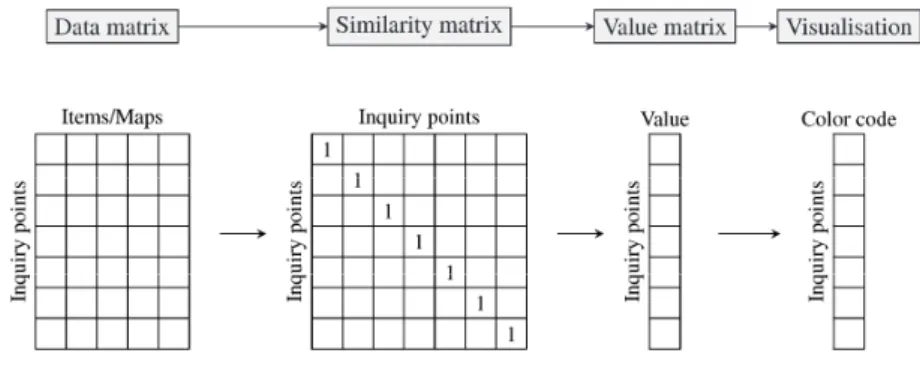
The idea behind traditional dialectometric methods is to aggregate infor-mation from as many maps as possible, in order to obtain a reliable generic picture of dialect landscapes. Following Goebl (e.g. Goebl 2010: 439), the traditional dialectometric pipeline consists of several steps (see Fig. 1). 4.2 The data matrix
The first step consists in aggregating information of several maps into aDATA MATRIX. The data matrix contains a row for each inquiry point and a column for each working map or linguistic item. The cells represent the variants that
_________________________
8Kellerhals (2014: 29) chose this approach in her dialectometric comparison between the SDS and SADS data.
9Multiple dominant variants occurred in 3.5% of cells, i.e. a comparable proportion as in the SDS data.
are used in a given inquiry point for a given phenomenon. The variants can be complete words, or pre-categorized variants. Furthermore, one may choose to deal with multiple mentions or even frequencies or probabilities, or limit oneself to a single mention per cell.
In our case, we build five data matrices, one for each linguistic level and one with the complete dataset. Our raw data consists of pre-categorized var-iants (as discussed above), and we allow them to occur as sets, in order to account for multiple dominant variants in the SADS data and for multiple mentions in the SDS data.
Fig. 1: The dialectometric pipeline.
4.3 The similarity matrix
In the second step, the data matrix is converted to a squareSIMILARITY MA-TRIXwith as many rows and columns as there are inquiry points. For each pair of inquiry points, a similarity value is computed by comparing the two corresponding rows of the data matrix. The simplest algorithm, known as Relative Identity Value (RIV, see Goebl 2010: 439) computes, for each pair of inquiry points, the proportion of cells in which the mentioned values are identical.
The RIV is ideal for datasets that do not contain multiple answers. How-ever, as mentioned above, the digitized SDS maps sometimes contain multi-ple answers for a given word at a given inquiry point, just like the SADS items may contain variants that are equally dominant. In earlier work on SDS data (Goebl et al. 2013), the multiple answers were reduced to single answers by removing secondary variants were these could be identified, and by ran-domly removing variants otherwise.
Here, we have chosen to extend the RIV measure to take into account mul-tiple answers, by treating every cell of the data matrix as a set that may con-tain zero, one or several variants. Measuring the similarity between sets is a thorny issue as the underlying linguistic assumptions are not quite clear (Goebl 2011), but several proposals have been made to deal with this phe-nomenon (e.g. Nerbonne & Kleiweg 2003). We have chosen the Jaccard sim-ilarity coefficient (Jaccard 1912), which defines the simsim-ilarity between two sets as the size of their intersection divided by the size of their union. The Relative Jaccard Similarity Value (henceforth RSVJaccard) of two rows A and B of length n is thus computed as follows:
Jaccard( , , ) =∑ Jaccard( , )
where
Jaccard( , ) =| ∩ | | ∪ |
In other words, RSVJaccard is an extended version of RIV that is able to deal with multiple answers.10
4.4 Value matrices
In the third step, the similarity matrix is condensed into aVALUE MATRIX, with the goal of having one single value per row. Different values emphasiz-ing different aspects of the spatial distribution of dialects have been proposed. One possibility is to select one column of the similarity matrix. This yields similarity maps relative to the selected inquiry point. Examples of such maps are shown in Goebl et al. (2013). Another possibility is to compute a statisti-cal parameter of the inquiry point such as the mean, the standard deviation or the skewness (see below).
Another idea is to group (or cluster) inquiry points with resembling simi-larity distributions using hierarchical clustering algorithms (e.g. Shackleton Jr. 2007; Nerbonne & Heeringa 2010; Goebl 2010). We present such experi-ments below.
_________________________
10Other similarity measures like Hamming distance, the Dice similarity coefficient or the overlap coefficient, may be used instead. Experiences with our datasets have shown negligible differences in terms of local incoherence between these measures, but rather large improvements with respect to standard RIV applied on randomly reduced multiple variants.
In the following we also present some correlative analyses. The goal of these analyses is to compare two similarity matrices row-wise in order to see how well they correlate. The matrices may either be linguistic similarity trices (e.g. to compare phonology with syntax) or geographic similarity ma-trices (e.g. to compare phonology with distance as the crow flies). The results of these correlative analyses may either be presented globally (i.e. as a single correlation score for each pair of matrices), or as maps. In the latter case, a value matrix is built on the basis of the row-wise correlation scores.
4.5 Visualization
In the fourth step, the value matrix is visualized, typically using Voronoi polygons in different colors11(Goebl 1984: 90–92) drawn around each
in-quiry point.
In the case of cluster analyses, each cluster number is associated with a clearly distinguishable color. However, if the value matrices contain real-val-ued scores (which is the case for statistical parameters and correlation scores), the visualization is more difficult. While it would be possible to cal-culate the color hue directly from these scores, the resulting maps would be difficult to read, since the exact differences between color hues are hard to distinguish. Therefore, the values are grouped into a small number of classes and each class is assigned a unique color. Goebl (1984: 93–97) has proposed and used two major classification techniques: MEDMW and MINMWMAX. We slightly depart from these techniques and use another classification tech-nique that is more popular in geostatistics, namely Jenks’ natural breaks clas-sification method (Jenks 1967). This technique works very similarly to Ward’s algorithm for hierarchical clustering, except that it is applied on the value matrix instead of the similarity matrix (see Section 5.1): when given a predefined number of classes, it defines the classes so that the variance within classes is reduced and the variance between classes is maximized. We ob-tained good results with 10 classes, which were mapped using a color ramp ranging from red to blue.12
_________________________
11For more detailed information on Voronoi diagrams see Aurenhammer (1991). 12Goebl (1984: 97) notes that Jenks’ algorithm does not take into account the mean value of the distribution when grouping and that its failure to do so results in disparate results. We have not observed such radical differences in the visualization when comparing the different algorithms.
55 DDaattaa aannaallyyssiiss
5.1 Data consistency and spatial autocorrelation
Before applying the whole dialectometric pipeline to visualize dialect pat-terns, we would like to compare our different datasets at the levels of the data matrix and the similarity matrix.
An interesting property of the data matrix is Cronbach’s alpha (Cronbach 1951; Heeringa 2004). Cronbach's alpha is a coefficient of consistency that tells us to what extent the different variables of the data matrix show the same distribution. If all variables have a similar geographic distribution of variants, the value of Cronbach’s alpha is 1. If all variables show different inconsistent geographic distribution patterns, the value is 0. A generally accepted thresh-old for good data consistency is 0.7 (Nunnally & Bernstein 1994).
Table 2: Cronbach’s alpha values for the data matrices of different linguistic levels.
Linguistic Level Cronbach’s Alpha
Morphology (118 variables) 0.93
Phonology (100 variables) 0.89
Lexis (64 variables) 0.89
Syntax (68 variables) 0.81
All levels (350 variables) 0.97
The five data matrices show Cronbach’s alpha values that all lie above the threshold of 0.7. The lowest value is obtained with the syntax dataset.
It is also useful to compare the different datasets with respect to their spa-tial autocorrelation. The principle of spaspa-tial autocorrelation has been adapted to dialect data by Nerbonne and Kleiweg’s Fundamental Dialectological
Postulate, which we already discussed in Section 2. We show two measures
of this postulate. First, we compute correlation scores between the linguistic similarity matrices and geographical distance matrices as the crow flies.13For
this, we use the Mantel test (Mantel 1967) with Pearson’s correlation coeffi-cient. Second, we compute local incoherence scores. Local incoherence (Ner-bonne & Kleiweg 2007) is based on the idea that spatial autocorrelation
_________________________
13To avoid negative correlations, we convert the linguistic similarity matrices into lin-guistic distance matrices, where each distance value corresponds to the complement to 1 of the similarity value.
should hold locally, so that differences between locations geographically far apart are discarded because these are mostly coincidental. Small local inco-herence values mean better coinco-herence and therefore better dialect measure-ments.
Table 3: Correlations between geographic distances (as the crow flies) and linguistic distances from different linguistic levels. The correlations and variances are com-puted using a Mantel Test with a simulated p-value (999 repetitions) < 0.001. For correlation and variance, higher values are better; for local incoherence, lower val-ues are better.
Linguistic Level Correlation (r) Explained Variance
(r2x 100) Local Incoherence
Geography ~ Morphology 0.82 68% 0.71
Geography ~ Phonology 0.72 52% 0.81
Geography ~ Lexis 0.77 59% 0.81
Geography ~ Syntax 0.64 41% 2.64
Geography ~ All levels 0.82 68% 0.56
The two measures show similar tendencies, but also some surprising differ-ences. Morphology correlates best with geography, nearly as well as the com-plete dataset. This is backed by the fact that the morphology subset is the largest. The syntax data shows lower spatial autocorrelation than the other levels and a proportionally much higher amount of local incoherence. This can be interpreted as a tendency of syntax to form larger dialect areas whose internal variation is not spatially autocorrelated. Therefore, it is difficult to obtain good correlations at the local level, but easier at a larger scale. 5.2 Cluster analysis
In order to get an idea of the geographic structures that are defined by the SDS and SADS data, we performed hierarchical cluster analyses of our whole dataset as well as of the different subsets. Cluster analyses are used in various disciplines and have become a standard procedure in dialectometry. The basic idea of all types of cluster analysis is to group variables in such a way that all members within a group are similar to each other but very different from members of different groups. This grouping (or clustering) is carried out in a stepwise process where in each step the two items or groups which are the most similar to each other are grouped together. This stepwise process results in a tree-like structure called dendrogram.
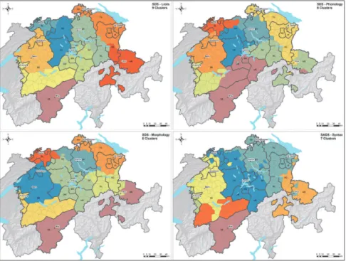
First, we will take a look at the geographic classification of dialect areas obtained by an analysis of the complete dataset. For this purpose we create a similarity matrix (cf. section 4.3) for our 377 places of investigation using all 282 maps from the SDS as well as the 68 variables from the SADS; i.e. a total of 350 working maps. We then perform a hierarchical cluster analysis using Ward’s minimum variance method (Ward 1963). This method tends to build clusters of similar size and has proven itself in practice (Gries 2008: 305). As in hierarchical cluster analyses the number is not specified in ad-vance, it is often not easy for the investigator to choose an appropriate num-ber of groups for the further discussion. While generally there is no single “best” number of clusters since this number may depend on specific ques-tions of the researcher with respect to the data, there are several ways to op-timize the number of groups (Everitt et al. 2011: 95). One possibility is to cut the dendrogram at a certain height where a large change in fusion levels can be observed. This method is “sometimes termed the best cut” (Everitt et al. 2011: 95). Of course, an appropriate number of groups can also be deter-mined on the basis of specific research questions. In Swiss German dialec-tology, claims have been made about large-scale dialectal divisions such as a north-south division or a west-east division (Haas 2000, Hotzenköcherle 1984). In our case it is especially interesting to compare these observations from traditional dialectology with the results of the dialectometric analyses. Therefore we take a look at the most large-scale clustering (i.e. two groups) and see how the dialectal landscape changes when we successively increase the number of clusters to three and four. Additionally, we compare these macro-structurings with a more fine-grained division of the data into ten groups, determined using the best-cut method. The items of each group are then coded in different colors and mapped to a Voronoi diagram where each polygon represents one survey location. It is important to note that the colors are only selected to distinguish between the clusters; i.e. similar colors do not represent linguistic similarity. The result is depicted in Fig. 2.
For a better comparison between the dialectal landscape and the political structure, the cantonal borders are included in the maps. Moreover, we added an example of the so-called Brünig-Napf-Reuss line (Weiss 1947) on the three-cluster map. This line stands for a number of cultural differences which separate Western from Eastern Switzerland and which often coincide with dialect isoglosses. For our purposes we chose the distribution of French and German playing cards, following Weiss (1947: Fig. 12).14
_________________________
14The choice of this border is somewhat arbitrary and shall only serve for illustration purposes. However, an inspection of the maps in Weiss (1947) reveals that many cultural customs share similar west-east distributions which are divided along a line that roughly
Fig. 2: Cartographic visualization of a hierarchical cluster analysis for the complete dataset (350 working maps). Similarity measure: RSVJaccard; cluster algorithm: Ward’s method. Brünig-Napf-Reuss line on upper right-hand map adapted from Weiss (1947: Fig. 12)
As the maps show, all clusters ‒ independently of the number of groups ‒ form homogeneous dialect regions. This result is not trivial since the cluster-ing algorithm does not take the geographic coordinates of the survey points into account but only their linguistic similarity. In this respect our analyses show that the Fundamental Dialectological Postulate apparently holds true for Swiss German dialects.
If we take a look at the upper left map, which shows a division into two clusters, we can observe a general west-east division of the dialectal land-scape, with major parts of the canton of GrisonsGRbelonging to the western cluster.15Moreover, the borders between the clusters coincide ‒ at least partly _________________________
runs from the Brünig pass across the Napf Mountain to the river Reuss in Northern Swit-zerland.
15The official abbreviations of the Swiss cantons are mentioned in small capital letters; the geographic localizations of the cantons can be looked up in Fig. 2 and 3.
‒ with the cantonal borders. While the cantons of ZurichZHand GlarusGL entirely belong to the blue, eastern cluster, we see that the neighboring can-tons of ZugZGand Uri URas well as large parts of the canton AargauAG belong to the western, red cluster. However, this convergence of cantonal and cluster borders does not hold true for all regions, as the example of the canton SchwyzSZillustrates.
The upper right map shows a solution of three clusters, where the western cluster is subdivided into two separate groups. Interestingly, the “new” bor-der between the two western clusters evidently coincides largely with the Brünig-Napf-Reuss line which, in turn, corresponds mostly with the political borders between the western cantons of BernBEand ValaisVSand the neigh-boring eastern cantons. If we consider other cultural west-east divisions as discussed in Weiss (1947), we see that most of the borders are situated within or along the central dialect group in our three-cluster map (see especially Weiss 1947: Fig. 9 and 16). The often postulated north-south partition of our research area, which for a long time was considered the most important dia-lect division in German-speaking Switzerland (since it coincides with the subdivision into High and Highest Alemannic), becomes apparent only in the next map, the four-cluster solution, where the canton of ValaisVS– together with GrisonsGR– is separated from the northern part.
Since it is not possible in this context to compare all numbers of clusters and the resulting geographic patterns with each other, we will finally take a look at a ten-cluster solution, which is visualized in the lower right map. If we compare it to the four-cluster map we can observe that each of the north-ern clusters is subdivided along a line which coincides to large parts with the topography and separates clusters situated in the northern lowlands from those located in the southern mountainous regions.
Without going too much into detail, we can sum up that both north-south and west-east divisions can be found as a result of our cluster analysis, with the west-east divisions being more important as they can already be observed for the more general geographic patterns with few clusters. This result con-firms Haas’ claim that the most profound dialectal differences within Ger-man-speaking Switzerland are not to be found between north and south – as has been stated in older dialectological research – but between west and east (Haas 2000: 63). Furthermore, the cantonal borders seem to play an important role for the dialectal landscape as they often coincide with the borders be-tween the clusters. On closer examination we can observe another distinction between the western and eastern part of German-speaking Switzerland: in the West, we find a lot more agreement between cantonal and cluster borders than in the East. This contrast also corresponds with Hotzenköcherle’s (1984: 61) characterization of the western part as more homogeneous, which is due to the long-lasting influence of Bern. On the other hand, he describes the East
as more fragmented, since Zurich started to become influential only later in history (Kelle 2001: 18).
While the cluster analysis of the complete dataset provides interesting in-sights into the Swiss German dialectal landscape, it does not tell us anything about the geographic patterns that result from the different linguistic levels. In the following, we take a look at the results of the cluster analyses of the four subcorpora. Since it is not possible to visualize various numbers of clus-ters for each of the linguistic levels, we restrain ourselves to one cluster so-lution per level. To this end, we apply the best cut method described above and select an optimal number of clusters for each individual level. Finally, we use nine clusters for the lexical data, eight clusters for both the phonolog-ical and morphologphonolog-ical subsets and seven clusters for the syntax data. The corresponding maps are shown in Fig. 3.
Fig. 3: Cartographic visualization of a hierarchical cluster analysis for different lin-guistic levels (lexis: 64 working maps; phonology: 100 working maps; morphology: 118 working maps; syntax: 68 working maps). Similarity measure: RSVJaccard; cluster algorithm: Ward’s method.
The visualizations of the cluster analyses of the four linguistic levels natu-rally show similarities with the result of the analysis of the complete dataset.
In all four maps, the eastern border of the canton of BernBEbecomes (more or less) apparent as well as the western border of the canton of ZurichZH. However, there are some characteristic differences between the maps, some of which will be discussed in the following:
‒ While for the lexical, phonological and morphological data the Basel re-gion (bs, bl) forms a separate cluster, it does not appear on the syntax map. Instead, the Northwest is divided into two parts both of which belong to a larger area that extends further to the South.
‒ For the lexical and the syntactical datasets, the canton of ValaisVSforms a distinct dialect region. On the level of phonology, this region is much larger and includes parts of the Bernese Highlands, the cantons Obwalden OW, NidwaldenNWand UriURas well as some locations in GrisonsGR. On the morphology map, the canton of ValaisVSis distinct from the neigh-boring cantons in the North but also clusters – to a much larger extent – with places in GrisonsGR. This similarity between the dialects of Valais VSand GrisonsGRis well known in Swiss German dialectology and can be explained by the so-called “Walser migrations” that started in the Mid-dle Ages and during which settlers from the Wallis (the German name for Valais) brought their dialects to the canton of Grisons (and other regions outside of Switzerland).
‒ While for lexis, phonology and morphology the Bernese Highlands (i.e. the southern part of the canton BernBE) form a cluster with the canton of FribourgFR, they are separated on the syntax map. This is especially re-markable since the clusters for the syntax data generally appear to be larger than for the other levels and the Ward algorithm used in our analysis tends to generate clusters of similar size. We can therefore conclude that Fri-bourgFRforms a syntactically very distinct region – a result which is ac-tually in line with previous findings based on SADS data (Bucheli Berger 2010; Stoeckle 2016).
‒ While the clusters for the SDS maps appear to be of similar size and gen-erally are distributed equally over the research area, on the syntax map we only find three large clusters which dominate the northern region. Indeed, in many studies based on SADS data geographic distributions of great re-semblance with the three big northern clusters have been detected, mostly displaying a west-east division between the dominance zones of two vari-ants (e.g. Seiler 2004; Glaser 2014). The fact that in the cluster analysis we find three big areas is probably to be explained by different locations of isoglosses on the west-east axis. Moreover, the syntax map shows a number of outliers, i.e. locations which are surrounded by places
belong-ing to a different cluster. If we specifically compare the dialectal classifi-cation of the (North-)East, we find that it is divided into several smaller areas for the levels of lexis, phonology and morphology, whereas it forms one large area for the syntactic level.
Based on our observation of the maps for the four linguistic levels we can draw the preliminary conclusion that the lexical, phonological and the mor-phological level appear to be similar to each other as well as to the complete dataset, while the syntactic level displays the most differences. However, this interpretation is based on mere visualization of the geographic patterns rather than on statistical evidence. Therefore, we discuss the results of a correlation analysis in order to support our hypotheses in the following chapter.
5.3 Correlations
One of the goals of our article is to compare the different linguistic levels with each other and to analyze how much each of them contributes to the geographic classification based on the complete dataset. Therefore, we com-puted correlations between the different subsets as well as between each sub-set and the complete data. The results are summarized in Table 4.
Table 4: Correlations between aggregated data from different linguistic levels. Sim-ulated p-value (999 repetitions) < 0.001.
Linguistic Levels Correlation (r) Explained variance (r2x 100)
Complete Data ~ Morphology 0.95 89%
Complete Data ~ Phonology 0.93 86%
Complete Data ~ Lexis 0.92 85%
Complete Data ~ Syntax 0.80 64%
Morphology ~ Lexis 0.84 70% Phonology ~ Lexis 0.82 67% Phonology ~ Morphology 0.81 66% Syntax ~ Lexis 0.71 50% Syntax ~ Morphology 0.69 47% Syntax ~ Phonology 0.66 43%
The upper part of the table presents the correlations of the individual linguis-tic levels with the complete dataset. All correlations are highly significant and generally have high coefficients, which is not surprising since all linguis-tic levels are subsets of the complete data and thus not independent. However, as in the previous analyses, we can observe differences between the four lin-guistic levels with syntax differing most from the other levels. The morpho-logical level has the strongest association with the complete data (89% of explained variance) followed by phonology (86%) and lexis (85%). The syn-tactic level only accounts for 64% of explained variance. One explanation could be the relatively low number of syntax maps (n=68) compared to pho-nology (n=100) or morphology (n=118). On the other hand, only 64 lexical maps are included in the analysis, which correlate to a much higher degree with the complete dataset than the syntactic maps. This suggests that the syn-tactic level indeed shows different patterns than the other linguistic levels. The lower part of Table 4 presents the correlations of pairs of linguistic levels. Compared to the correlations discussed above, the coefficients are smaller, which is expected as the different levels and the corresponding distance ma-trices can be considered independent of each other.16However, the smallest
coefficient is r=0.64 and all correlations are significant at the 0.001 level, so we can state that the linguistic levels are generally highly associated with each other. Overall, we find a pattern similar to the other analyses: While all SDS datasets correlate highly with each other (especially the lexical level with the other levels), the syntactic level shows much lower associations with the other levels.
If we compare our results to related surveys, we find that the associations among the different linguistic levels in German-speaking Switzerland are sur-prisingly high. In her study on Tuscan dialects, Montemagni computes the “correlation between phonetic and morpho‒lexical distances [which] turns out to be 0.4125, with only 17% of explained variance” (Montemagni 2008: 143). Spruit et al. (2009) analyze the associations among the linguistic levels of pronunciation, lexis and syntax for Dutch dialects and obtain correlation coefficients of 0.496 for lexis ~ syntax, 0.617 for pronunciation ~ lexis, and 0.648 for syntax ~ pronunciation.
_________________________
16Strictly speaking they are not totally independent since – apart from the syntax data – the data originates from the same informants. There are also some instances where vari-ation in one level could be explained by another level such as the (lexical) varivari-ation be-tween bald and baud ‘soon’ (besides variants such as glii; see SDS map VI.30), which in fact can be reduced to the vocalization of /l/. However, these cases are rather rare in our data, and since every variable was only used in one subset of the data, they can be treated as independent.
It is also interesting to compare the associations between linguistic levels and geographical distance with the cited studies on Tuscan and Dutch. Recall that we obtained correlation coefficients between 0.64 (geography ~ syntax) and 0.82 (geography ~ morphology); see Table 3. For Tuscan, the respective coefficients are 0.6441 for the correlation between geography and morpho-lexical distances and only 0.1358 for the correlation between geography and phonetic distances (Montemagni 2008: 145). For Dutch, Spruit et al. (2009: 1639) report correlation coefficients of 0.575 (lexis), 0.669 (syntax) and 0.685 (pronunciation). The very high correlations between linguistic levels and between dialect and geographic distances found in our data can presum-ably be accounted for by the fact that the dialects in German-speaking Swit-zerland are still very vivid. This is all the more surprising as we would have expected the mountainous topography of Switzerland to have a negative ef-fect on correlations compared e.g. to the topographically less complex Neth-erlands: in mountain areas, as-the-crow-flies distances seem a rather inade-quate measure.17
5.4 Parameter maps
The correlation analysis has already shown that the datasets from different linguistic levels behave differently in terms of the linguistic landscapes they define. Here, we add a more thorough analysis that compares the linguistic levels according to various statistical parameters, following Goebl (1984). For this purpose, we discuss the three parameters arithmetic mean, standard
deviation, and skewness. These properties are calculated independently for
each inquiry point on the basis of its similarity value distribution. We start by illustrating these properties by looking at four inquiry points: Fribourg, Visp (located next to Brig), Zurich and Chur. Fig. 4 shows four histograms, which represent the distribution of similarity values for each of the four points.
The first property to be read off these histograms is the arithmetic mean: it corresponds to the similarity value (as indicated on the X-axis) that is lo-cated at the peak of the normal distribution. These values lie around 0.5 for Fribourg and Visp, at 0.64 for Zurich, and at 0.57 for Chur. In the resulting map, low values would be colored blue, and high values red.
The standard deviation of a distribution measures the amount of disper-sion, or in other words, whether the shape of the distribution is sharp or flat. Standard deviation values close to 0 indicate that the similarities are gathered close to the mean value, whereas high standard deviation values indicate that the similarities are spread out more widely below and/or above the mean. In
_________________________
17 Experiments with different definitions of travel times have been conducted by Jeszenszky and Weibel (forthc.) for Swiss German syntax data.
our examples, Fribourg and Chur have the lowest standard deviation values (around 0.095), whereas Visp has a slightly higher value (0.11) and Zurich has the highest one (0.13); however, all values are quite low. Thus, Fribourg and Chur would be colored in blueish hue, Visp and Zurich in greenish hue.
Fig. 4: Histograms for the four inquiry points Fribourg, Visp, Zurich and Chur, us-ing the similarity distributions of the complete dataset. The blue line indicates the normal distribution.
The standard deviation indicates whether the similarity distribution is sharp or flat, but it does not indicate whether this distribution leans towards the left or towards the right side. This asymmetry is measured by another property called
skewness. Positive skewness values (i.e. between 0 and +1) stand for similarity
distributions skewed towards the right: the mass of the distribution is located to the left of the mean and the distribution has a long tail to the right. Con-versely, negative skewness values (i.e. between –1 and 0) stand for similarity distributions skewed towards the left. In our examples, Fribourg and Visp have positive skewness values (1.3 and 2.1 respectively). Zurich and Chur roughly have an equal amount of probability mass on the left and on the right side of the mean; their skewness values are thus close to 0 (0.2 and 0.3 respectively). On the maps, negative values are colored in blue, positive values in red.
It should be noted at this point that our main interest lies in the geographic patterns resulting for each linguistic level rather than in the exact comparison of the parameter values. Therefore we use an individual scale for each level, which means that the colors on each map can only be interpreted relative to the scale for the respective level, but not between levels. For example, a skewness value of 0 can be associated with red color in one linguistic level (if no inquiry point of that level has negative skew) but with blue color in another level (if no inquiry point of that level has positive skew).
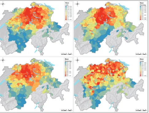
5.4.1 Arithmetic mean
From a dialectological point of view, the arithmetic mean indicates how well an inquiry point communicates with its surroundings. High mean values are usually found in central places of the investigated area, whereas low mean values tend to occur in peripheral areas (see for example Goebl 1984: 148). Fig. 5 shows the mean similarity values for the four linguistic levels, where high mean similarities are displayed in red and low mean similarities in blue.
Fig. 5: Mean similarity values for different linguistic levels (lexis: 64 working maps; phonology: 100 working maps; morphology: 118 working maps; syntax: 68 working maps). Similarity measure: RSVJaccard; classification algorithm: Jenks’ natural breaks, 10 classes.
The lexis, phonology, and morphology maps show similar pictures. Indeed the reddest areas correspond to the most central area of the lowlands area north of the Alps (this lowlands area ranges roughly from Fribourg to St. Gallen). The red area is most compact in morphology, whereas it extends further eastwards in lexis and phonology. The syntax map differs from the other maps in two aspects. First, the computed mean similarity values are much higher (see legends of Fig. 5), which means that the syntactic questions are less able to discriminate the different dialects. Second, there are fewer perceptible differences within the lowlands area, and high mean similarities are found throughout the investigated area, from its westernmost to its east-ernmost parts. However, all four maps show low mean similarities in the pe-ripheral zones of Valais, Fribourg and Grisons, which is in line with the gen-eral interpretation. In the SDS maps, these blue zones sometimes extend to the Northwest, sometimes to the Northeast, sometimes to Central Switzerland (just south of Lucerne).
5.4.2 Standard deviation
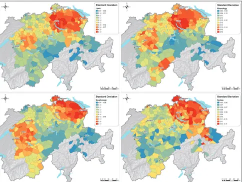
Linguistically, high standard deviation values indicate the concentration of centripetal tendencies, or distinct dialect zones (Goebl 1984: 167). Goebl also notes that linguistic areas often tend to have several such zones, which are separated from each other by transition zones with low standard deviation values. Fig. 6 shows the standard deviations of the similarity distributions at each inquiry point, with high standard deviation values (dialect centers) in red and low standard deviation values (transition zones) in blue.
On all four linguistic levels, the highest standard deviation values are ob-served in the Northeast, in a region ranging from Zurich (sometimes includ-ing it) to Lake Constance. Generally, the Northeast has been characterized as innovative and open (Weiss 1947: 162), but the image conveyed by the stand-ard deviation maps is rather one of a strong, internally coherent dialect area that may or may not be innovative in comparison to its surroundings. Inter-estingly, we find support for our controversial interpretation in Hotzenköch-erle (1984: 95–100) who discusses the ambivalent character of the area by providing examples for both innovative and conservative linguistic features. On all maps except syntax, another – smaller – zone with high standard de-viation values appears around Bern. This suggests that the dialectal organi-zation of Lowlands Swiss German is bipolar, with the two poles lying in Zur-ich and Bern. Interestingly, the city of Basel, larger than Bern in terms of inhabitants, does not show the same behavior. Also, centripetal tendencies are currently not observed in Central Switzerland, suggesting that the city of Lucerne has (yet) limited influence on its surrounding dialects.
Fig. 6: Standard deviations of the similarity distributions for different linguistic lev-els (lexis: 64 working maps; phonology: 100 working maps; morphology: 118 working maps; syntax: 68 working maps). Similarity measure: RSVJaccard; classi-fication algorithm: Jenks’ natural breaks, 10 classes.
The phonology map shows a third central zone in Valais (around Brig), sug-gesting that the Valais dialect, separated through the Alpine main ridge, de-velops independently of northern influences. Finally, the scattered red dots in the Southeast of the syntax area (around Chur) are probably an effect of the particular language situation in that area, where southwestern Walser dialects meet northeastern dialects; note however that the absolute standard deviation values of these points are relatively low and would have been displayed in green or yellow if using the scales of the other levels
5.4.3 Skewness
Positive skewness values stand for peripheral areas with weak typological links to the rest of the dialect area; Goebl (1984: 167) characterizes such areas as “minorities within the majority”. Negative skewness values indicate dia-lectal transition zones. Fig. 7 shows the skewness maps for the four linguistic
levels. Positive skewness values are visualized in red, negative skewness val-ues in blue.
Fig. 7: Skewness values of the similarity distributions for different linguistic levels (lexis: 64 working maps; phonology: 100 working maps; morphology: 118 working maps; syntax: 68 working maps). Similarity measure: RSVJaccard; classification algorithm: Jenks’ natural breaks, 10 classes.
On all linguistic levels, the Valais region stands out as a conservative dialect area with little contact to the other regions. This area sometimes extends to the Bernese Highlands and to Fribourg (lexis, phonology, syntax) and to Cen-tral Switzerland (lexis, phonology). Another conservative dialect area is found in parts of the Walser dialect area in the Southeast. Finally, the Basel region shows high skewness values as well, with the exception of the syntax data. These results may also explain the absence of this region as a conver-gence pole: it may not communicate enough with the surrounding regions to be able to figure as a central pole. However, this effect is not visible in the syntax data.
In general, all maps show low values on a stretch ranging from the east of Basel to Chur, avoiding Zurich by the North or the South, but note again the differing ranges of skewness values (between ‒1.30 and 2.09 in the syntax
map, but only between ‒0.34 and 1.67 in the phonology map). Interestingly, the blue band of low values closely follows the first, most important border obtained in the cluster analysis (see Fig. 2). This concording evidence from two different methods suggests that the Swiss German dialect landscape can be divided into a smaller northeastern and a larger southwestern area. Parts of this blue stretch are known to be dialectal transition zones. For example, Hotzenköcherle (1984: 79) characterizes the Aargau as “highly labile” in terms of dialects, whereas Trüb (1951, cited in Hotzenköcherle 1984: 112) emphasizes the “vibrations” and the inconsistency of the Walensee region. To sum up, the four linguistic levels produce rather similar dialect land-scapes, which was not necessarily expected for the syntax dataset. Whereas the syntax map differs a lot from the other ones regarding the mean value distribution, the differences are much less marked in the standard deviation and skewness analyses. The most obvious difference lies in the less promi-nent linguistic differentiation within the lowlands area north of the Alps. Whether this is a true difference between syntax and the other linguistic lev-els, or rather a result of dialect convergence taking place since the SDS in-quiries remains to be investigated. Presumably, both factors are involved.
66 DDiissccuussssiioonn
6.1 A short characterization of the Swiss German dialect landscape
In this final section of the article, we connect the different parts of our anal-yses to characterize (some parts of) the Swiss German dialect landscape. To this end, we use the classification resulting from the cluster analysis and char-acterize the different areas on the basis of the statistical parameters presented in the preceding section. Since we performed hierarchical cluster analyses with various datasets ‒ i.e. the complete dataset as well as the different lin-guistic levels – and each of these analyses yields a large number of cluster solutions, we have to limit ourselves to one dialect classification. We there-fore choose the map resulting from the cluster analysis of the complete da-taset with 10 clusters, as depicted in Fig. 2, and select some “interesting” dialect areas for illustration purposes.18
The first area we characterize stands out in almost all cluster analyses (ex-cept for the syntactic level) and is located in the Northwest around the two half-cantons of BaselBS/BL, covering also small parts of the cantons of Solo-thurnSOand AargauAG. In this area, the lexical, phonological and, to a lesser extent, the morphological levels exhibit a similar pattern: The low values for
_________________________
the arithmetic mean and the high positive skewness values suggest a dialec-tally isolated area with little linguistic levelling. On the syntactic level, how-ever, the area seems to be more integrated into the larger dialectal landscape, showing rather high mean values as well as negative values for skewness. As an ultimate result of this integration, the area diffuses into two larger areas. We also find descriptions of this area in the traditional dialectological litera-ture such as Hotzenköcherle (1984: 73–76) who states a close linguistic rela-tionship with the neighboring Alsatian dialect. For a closer dialectomectric examination, it would be interesting to include data from the Atlas
Linguis-tique et Ethnographique de l’Alsace (ALA; Beyer & Matzen 1969;
Bothorel-Witz et al. 1984) into our study.
In the Southwest, the canton of Valais vs forms a separate dialect area. This region is well-known for its linguistically conservative character and has been referred to a lot in the literature. Our data also suggests a straight-forward interpretation, which confirms these results: For all linguistic levels we find very low arithmetic mean values as well as very high positive skew-ness values, pointing to a rather isolated dialect area with very little linguistic compromise. Interestingly, the phonological level stands out in this context: On the one hand, the cluster is much larger compared to the other linguistic levels. On the other hand, we find an area with high standard deviation values in the northern Valais. These observations suggest that this southern cluster forms a separate dialect group with its own center, developing independently from the North.
The region which is often referred to as Central Switzerland and which includes the cantons of ObwaldenOW, NidwaldenNWand UriURas well as parts of ZugZGand SchwyzSZis slightly more difficult to characterize. For this area we found low standard deviation values as well as rather high posi-tive skewness values with respect to all linguistic levels. These results sug-gest that the cluster forms a dialectal relic area with little dynamics which does not represent a distinct dialect center. Again, the phonological level shows some special characteristics: As discussed in the last paragraph, cen-tral Switzerland forms a cluster with the Valais region, which also becomes apparent in the distribution of the low mean values. Besides, the municipality of Engelberg in the canton Obwalden OW is an exception with respect to skewness: while being surrounded by places with very high positive skew-ness values (between 1.15 and 1.67), it only possesses a skewskew-ness value of 0.18, therefore representing a linguistically less isolated place within a relic area. The special status of Engelberg has already been discussed by Hotzen-köcherle (1984: 264), who gives a historical explanation as Engelberg used to be an independent principality for almost seven centuries. More recently, Bösiger & Schiesser (2014) showed that Engelberg is not only considered a
“special case” by dialectologists, but also regarded as linguistically peculiar by speakers from Engelberg and neighboring places.
As we have mentioned in the beginning of this paragraph, our selection of dialect areas to be characterized more deeply on the basis of the parameter maps was primarily made for illustration purposes. This does not imply that the other regions are less interesting (especially the dialect areas resulting from the cluster analyses for the individual linguistic levels), but to discuss all of them would go beyond the scope of this article. However, we hope to have shown how the combination of different methods can contribute to a better understanding of dialectal dynamics and diversity and of the relation-ship between language and geography in general.
6.2 Conclusion
The first goal of this article was to introduce the digital database which has been made available in the last years and which consists of dialect data from the two big Swiss German atlas projects SDS and SADS. We have presented methods to make these datasets comparable, and we hope to have shown that our data is well suited for dialectometric analyses.
In order to achieve our second goal, a dialectometric survey of Swiss Ger-man dialects, we performed various analyses. These not only confirm Ger-many findings from traditional dialectology – such as the two major geographical west-east and north-south divisions or the detection of more “conservative” southern dialects (especially in the Valais) – but more importantly allow for a more precise characterization of the dialectological landscape as well as for the comparison of the linguistic levels. Our results show that although we find many differences between the linguistic levels, they generally seem to be coherent. The divergences mostly affect (more or less important) details such as the precise course of cluster borders or the exact distribution of pa-rameter values. Looking at the general picture, we find some patterns that seem to be true for all levels. These include a high degree of agreement be-tween cantonal and cluster borders, a classification into more dynamic north-ern areas and more conservative southnorth-ern regions (although the west-east di-vision generally seems to be more important) and generally very high corre-lations with geography as well as between the linguistic levels. As we have stated earlier, this result is in line with the general observation that the dia-lects of Swiss German are – compared to other dialect areas – still very vivid, as they serve as the most important means of everyday communication.
However, among all linguistic levels it is syntax which shows the most differences. Generally, the distributions of the individual syntactic variables appear to be more large-scale and spatially less coherent; i.e. they do not gen-erate the same fine-grained, differentiated dialect divisions we find in other
levels. This is reflected in the fact that the syntax maps – both cluster and parameter maps – are more fragmented and it also becomes apparent in the “poorer” statistical values for Cronbach’s alpha, for the correlation with ge-ography and for local incoherence. Moreover, the syntactic level does not show some characteristics which are shared by the other levels like an even distribution of dialect areas or some characteristic dialect regions such as (North-)Eastern Switzerland, Basel or the Bernese Highlands together with Fribourg. These results are not surprising since the special status of (dialect) syntax with respect to geographic variation has often been discussed in the literature (e.g. Lötscher 2004; Glaser 2014). It has even been questioned whether dialect syntax shows any geographic variation at all since it hardly differs from standard syntax (Löffler 2003: 109). However, as our results suggest, syntactic variables clearly show patterns of geographic distribution, although differing from other linguistic levels. At the current state it is not clear whether these differences are due to syntax-specific properties or can be explained by the fact that SADS data were collected some 50 years after the SDS survey using different methods. Probably, both explanations account to some extent for the differences.
Acknowledgements
The authors would like to thank the Swiss National Science Foundation for supporting their research through the project “Modelling morphosyntactic area formation in Swiss German (SynMod)” (SNF Project no. 140716) as well as the University Research Priority Program “Language and Space” for granting Yves Scherrer a short-term fellowship at the University of Zurich. References
Aurenhammer, Franz. 1991. Voronoi diagrams – A survey of a fundamental geo-metric data structure. ACM computing surveys 23: 345–405.
Barbiers, Sjef, Hans Bennis, Gunther de Vogelaer, Magda Devos & Margreet van der Ham. 2005. Syntactic atlas of the Dutch dialects, vol. 1. Amsterdam: Am-sterdam University Press.
Beyer, Ernst & Raymond Matzen (eds.). 1969. Atlas linguistique et ethnographique
de l’Alsace, vol. 1. Paris: Editions du C.N.R.S.
Blancquaert, Edgard & Willem Pée. 1925–1982. Reeks Nederlands(ch)e
dialect-atlassen. Antwerpen: de Sikkel.
Bösiger, Melanie & Alexandra Schiesser. 2014. Der Engelberger Dialekt – ein Son-derfall. Ängelbärger Zeyt. Engelberger Jahrbuch 2015: 140–146.
Bothorel-Witz, Arlette, Marthe Philipp & Sylviane Spindler (eds.). 1984. Atlas
lin-guistique et ethnographique de l'Alsace, vol. 2. Paris: Editions du C.N.R.S.
Bucheli Berger, Claudia. 2008. Neue Technik, alte Probleme: Auf dem Weg zum Syntaktischen Atlas der Deutschen Schweiz (SADS). In Sprachgeographie
di-gital. Die neue Generation der Sprachatlanten, 29–44. Eds. Stephan Elspass &
Werner König. Hildesheim: Olms.
Bucheli Berger, Claudia. 2010. Dativ für Akkusativ im Senslerischen (Kanton Frei-burg). In Alemannische Dialektologie: Wege in die Zukunft. Beiträge zur 16.
Ar-beitstagung für alemannische Dialektologie in Freiburg/Fribourg vom 07.‒ 10.09.2008, 71–83. Eds. Helen Christen, Sibylle Germann, Walter Haas, Nadia
Montefiori & Hans Ruef. Stuttgart: Steiner.
Bucheli, Claudia & Elvira Glaser. 2002. The syntactic atlas of Swiss German dia-lects: Empirical and methodological problems. In Syntactic microvariation (Meertens Institute Electronic Publications in Linguistics 2), 41–74. Eds. Sjef Barbiers, Leonie Cornips & Susanne van der Kleij. Amsterdam: Meertens Instituut.
Chambers, Jack K. & Peter Trudgill. 2004. Dialectology, 2nd edn. Cambridge:
Cambridge University Press.
Cronbach, Lee. 1951. Coefficient alpha and the internal structure of tests.
Psy-chometrika 16: 279–334.
Embleton, Sheila. 1993. Multidimensional scaling as a dialectometrical technique: outline of a research project. In Contributions to quantitative linguistics.
Pro-ceedings of the first international conference on quantitative linguistics (QUAL-ICO), 267–276. Eds. Reinhard Köhler & Burghard B. Rieger. Dordrecht &
Bos-ton: Kluwer Academic Publishers.
Everitt, Brian S., Sabine Landau, Morven Leese & Daniel Stahl. 2011. Cluster
Analysis. 5thedn. Chichester, U.K.: Wiley.
Goebl, Hans. 1984. Dialektometrische Studien: Anhand italoromanischer,
rätoro-manischer und gallororätoro-manischer Sprachmaterialien aus AIS und ALF. 3 vols.
Tübingen: Niemeyer.
Goebl, Hans. 2005. La dialectométrie corrélative: un nouvel outil pour l’étude de l’aménagement dialectal de l’espace par l’homme. Revue de Linguistique
Ro-mane 69 : 321–367.
Goebl, Hans. 2010. Dialectometry and quantitative mapping. In Language and
Space. An International Handbook of Linguistic Variation. Vol. 2: Language Mapping (Handbücher zur Sprach- und Kommunikationswissenschaft 30.2),
433–457. Eds. Alfred Lameli, Roland Kehrein & Stefan Rabanus. Berlin/ New York: de Gruyter.
Goebl, Hans. 2011. Quo vadis, atlas linguistice? Einige wissenschaftshistorische und zeitgeistkritische Reflexionen zur atlasgestützten Geolinguistik. In
Sprach-kontakte, Sprachvariation und Sprachwandel, 5–27. Eds. Claudia Schlaak &