HAL Id: hal-03230523
https://hal.archives-ouvertes.fr/hal-03230523
Submitted on 20 May 2021
HAL is a multi-disciplinary open access
archive for the deposit and dissemination of
sci-entific research documents, whether they are
pub-lished or not. The documents may come from
teaching and research institutions in France or
abroad, or from public or private research centers.
L’archive ouverte pluridisciplinaire HAL, est
destinée au dépôt et à la diffusion de documents
scientifiques de niveau recherche, publiés ou non,
émanant des établissements d’enseignement et de
recherche français ou étrangers, des laboratoires
publics ou privés.
Modules for Photovoltaic Inverters Considering the
Inverter Mission Profiles
Mouhannad Dbeiss, Yvan Avenas, Henri Zara, Laurent Dupont, Franck Al
Shakarchi
To cite this version:
Mouhannad Dbeiss, Yvan Avenas, Henri Zara, Laurent Dupont, Franck Al Shakarchi. A Method for
Accelerated Aging Tests of Power Modules for Photovoltaic Inverters Considering the Inverter Mission
Profiles. IEEE Transactions on Power Electronics, Institute of Electrical and Electronics Engineers,
2019, 34 (12), pp.12226-12234. �10.1109/TPEL.2019.2907218�. �hal-03230523�
A method for accelerated ageing tests of power modules for
photovoltaic inverters considering the inverter mission profiles
Mouhannad DBEISS
1, 2, Yvan AVENAS
2, Henri ZARA
1, Laurent DUPONT
3, Franck AL
SHAKARCHI
11
FRENCH ALTERNATIVE ENERGIES AND ATOMIC ENERGY
COMMISSION-NATIONAL SOLAR ENERGY INSTITUTE (CEA-INES)
2
UNIV. GRENOBLE ALPES, CNRS, G2Elab
3SATIE IFSTTAR
1
Le Bourget du Lac, France ;
2Grenoble, France ;
3Versailles, France
T. +33 (0)4 79 79 21 44 | F. +33 (0)4 79 68 80 49
Mouhannad-Dbeiss@hotmail.com | yvan.avenas@g2elab.grenoble-inp.fr
Acknowledgments
This project has received support from the State Program Investment for the Future bearing the reference (ANR-10-ITE-0003)
Keywords
«Mission profile» «Renewable energy systems» « (VSC) Voltage Source Inverters» «Reliability» «Thermal cycling»
Abstract
This paper presents a new method for the accelerated ageing tests of power semiconductor devices in photovoltaic inverters. Mission profiles are analysed: output current and ambient temperature are extracted over several years from multiple photovoltaic plants located in France. It is then proposed to create a particular ageing profile which takes into account not only the different constraints of the application of the photovoltaic inverters (high-frequency switching and sinusoidal-shaped current), but also reproduces a typical profile of the output current of photovoltaic inverters. Similarly, the ambient temperature varies as in the real application. By applying current injections with relatively long durations, the DBC (Direct Bonded Copper) substrates and the coolers are subjected to high temperature swings. This method should show better representation of the thermal behavior of DC/AC inverters used in photovoltaic applications, and is expected to show more representative results than traditional power cycling, thus reducing the favoring of certain failure modes to the detriment of others.
1. Introduction
In photovoltaic systems, the DC/AC inverter has the highest failure rate, and the anticipation of its breakdowns is still difficult [1]. According to several recent evaluations, transistors contribute on average to 69% of the overall failure rate, diodes to 16%, capacitors to 14%, and magnetic elements to 1% [2].
Moreover, according to [3], power devices represent more than 30% of the total inverter’s failures, followed by the capacitors with a failure rate of approximately 18%. Failures of PV inverters can occur under non-intentional operations in islanding mode or under grid faults. It can also occur under normal operations due to several factors such as humidity, electrical overstress, temperature or other severe conditions. The most observed factors among those latter are related to the temperature, including peak temperature and temperature swings [1] [3]. In effect, the steady-state and cyclical temperature represent 55% of the stress sources [4].
[4] However, it can be found in [2] and [5] that the absolute temperature is not the dominant factor in the reliability performance, while thermal cycles contribute to a large percentage of the overall failure rate [6]. Hence, cyclic loads are more important than peak loads, especially because PV inverters often experience large temperature swings, due to variable solar irradiance and ambient temperature. In the case of high temperature variations, failures are usually induced by the mismatch in the coefficients of thermal expansion of the different materials in the chips and packages [2].
In this context, it is crucial to accelerate the ageing of the power modules to study their main failure modes. As a general rule, the accelerated ageing of power modules is carried out under aggravated conditions of current (Active Cycling) or temperature (Passive Cycling) in order to accelerate the ageing process. Unfortunately, when applying this type of accelerated ageing tests, some failure mechanisms that do not occur in the real application could be observed, while inversely, other mechanisms that usually occur could not be recreated [7].
This paper presents two methods of accelerated ageing of photovoltaic (PV) inverters’ semiconductors. Both are based on the analysis of real mission profiles: output current and ambient temperature data are extracted over several years from different photovoltaic power plants.
2 As represented in Fig. 1, a power losses estimation
model as well as a thermal model are used to estimate the junction temperature profiles, corresponding to different output current and ambient temperature profiles [8]. The 1st one corresponds to the real mission profiles, the 2nd one corresponds to accelerated ageing profile built with the 1st method, and the 3rd one corresponds to the accelerated ageing profile built with the 2nd method. In Fig. 1, 𝐼 represents the RMS current profile at the output of the inverter over a fundamental period 𝑇𝑜𝑢𝑡= 20 𝑚𝑠. 𝑃 is the semiconductor power
losses profile, 𝑇𝐽 the junction temperature profile, ∆𝑇𝐽
the temperature swings, 𝑇𝐽𝑀 the mean temperature of
each temperature swing, and 𝑇𝑎 the ambient
temperature.
Next, a cycle counting algorithm is appointed to extract the cycles from the junction temperature profiles, as well as the corresponding 𝑇𝐽 𝑀 and ∆𝑇𝐽 of
each extracted cycle. Then, the ageing profiles are refined according to the desired 𝑇𝐽𝑀 and ∆𝑇𝐽’s
distributions. Afterwards, a comparison is performed between the different profiles, regarding the distributions of ∆𝑇𝐽 and 𝑇𝐽𝑀. Finally, the tests’ duration is estimated using Palmgren-Miner rule with a lifetime estimation model.
Fig. 1: Full approach of the study
2. Methodology for accelerated
ageing profiles generation
2.1. Analysis of photovoltaics’ mission
profiles
The aim of this study is to create an accelerated ageing method, generating thermo-mechanical stresses in the semiconductors, while considering the photovoltaic application. Thus, mission profiles of inverters’ RMS output current and ambient temperature are extracted from four photovoltaic power plants, located in the south of France over three years: 2013, 2014 and 2015. The mean power range of the power plants is ~ 4 MW (16 MW maximum), each covering approximetaly 55000 m². Moreover, the mean power of the monitored inverters is approximetly 1 MW, while the data sampling rate of extracted mission profiles (800 MS each) is 1S/5s. Due to similarities within the data, one mission profile over a single year serves as an example in this paper. It is important to note that, in a
real reliability study, it would be necessary to study data over many years. Indeed, by using data over only 3 years, the profile could be largely modified by a singular event, for example a season that is cloudier than usual. However, because the present paper focuses on the methodology for obtaining an accelerated ageing mission profile, a study on over a relatively short duration (3 years) is proposed.
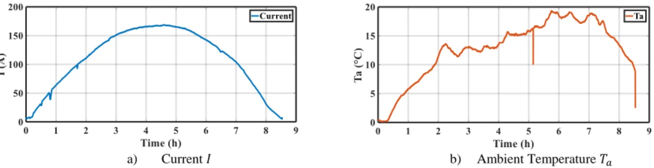
The profiles of the current and ambient temperature can show clear sky days as in Fig. 2, or cloudy days as in Fig. 3, with Fig. 3.a highlighted in Fig. 4. The variations of the current as represented in Fig. 3.a lead to numerous and sudden variations of semiconductors’ junction temperature during the day. These variations lead to semiconductors’ damages as found in the literature in the case of IGBT power modules [9] [10]. By analyzing the current profiles, several characteristics can be identified, as it will be presented in the upcoming sections. It should be noted that the values of certain parameters may depend on the power plant’s location and size. An analysis is thus required for each case.
a) Current 𝐼 b) Ambient Temperature 𝑇𝑎
3
a) Current 𝐼 b) Ambient Temperature 𝑇𝑎
Fig. 3: 𝐼 and 𝑇𝑎 mission profiles over a cloudy day
Fig. 4: Highlight on several current variations from Fig. 3.a
2.1.1. The shape of the current
As it can be noticed in Fig. 2.a, the shape of the RMS output current of the DC/AC inverter during the sunshine can be described by a mathematical equation as follows:
𝛼 ∙ 𝑠𝑖𝑛(𝑡) ∙ cos (𝑡) (1) where 𝑡 is a parameter that is time dependant, and α a variable that includes several parameters such as the geographical area, the orientation of the photovoltaic panels, and many others [11]. The number of sunshine hours depends on the season as well as on the geographical zone, while no current is produced by the PV panels during the night.
2.1.2. The diffuse current
When the sun is hided by clouds, the output current is proportional to the diffuse solar radiation. This latter -represented over one day in Fig. 5- results from diffraction of sunlight by the clouds and its scattering by various molecules and particles suspended in the atmosphere, as well as from its refraction by the ground. The global radiation is equal to the sum of direct and diffuse radiations, where diffuse radiation at a given moment is close to 10% of the global radiation. Hence, the current produced during the passage of clouds at a given moment is close to 10% of the total current that the PV panels produced directly before the passage of the clouds [12]. In other words, the amplitude of the current variation during the passage of clouds ∆𝐼 is equal to 90% of the current produced before the passage of clouds 𝐼𝐶𝑙𝑒𝑎𝑟.
Fig. 5: Solar radiation over one day
2.1.3. The slope of the current variations
During traditional power cycling tests, the variations of the current are abrupt, which may accelerate the damage in the module, potentially in a non-representative way. As far as we know, the current variations’ slope has never been studied in the literature, despite the fact that the thermo-mechanical stress may depend on it. Thus, it was an interesting fact, during this study to consider the current variations slope during the accelerated ageing of the semiconductor devices. In order to build a profile that accelerates the ageing of the power modules of the DC/AC photovoltaic inverter, slight current variations were neglected. Thus, only the current variations higher than ∆𝐼𝑚𝑖𝑛 leading to ∆𝑇𝐽≥30 𝐾 were retained, where the value of 30 𝐾 was arbitrarily selected. The value of ∆𝐼𝑚𝑖𝑛 can be
determined using a thermal model. Fig. 6 illustrates the extraction of current’s considerable variations over several days represented with a red line.
Fig. 6: Extraction of current’s considerable variations
As shown in Fig. 6, the variation’s speed of the RMS current value can be very fast due to cloud passageway. Actually, it depends on the speed of the wind and hence varies from a season to another. It also depends on the size of the photovoltaic power plant and its location. Considering the available data, the maximum slope of these sudden variations is estimated to be:
4
∆𝐼
∆𝑡
= 0.15 ∙ 𝐼𝑀𝐴𝑋 (A/s) (2) where 𝐼𝑀𝐴𝑋 is the maximum RMS current reached
during one year. This slope is obtained through statistical studies carried out on current measurements from photovoltaic power plants located in the south of France, which may be different in another geographical zone. However, since all the PV plants are located in the south of France and have approximatively the same surface, very close current slopes were obtained for the studied PV plants over the different years. These slopes vary in the south of France from 0.05∙ 𝐼𝑀𝐴𝑋 to 0.15 ∙
𝐼𝑀𝐴𝑋, thus in order to allow for the acceleration of the
ageing tests, the maximum value of 0.15 ∙ 𝐼𝑀𝐴𝑋 was
chosen in the example presented in this paper.
2.1.4. Delays between the current variations
As mentioned previously, slight current variations are neglected. Thus only the delays between the current variations higher than ∆𝐼𝑚𝑖𝑛 are considered. The
histogram illustrated in Fig. 7 represents the percentage of occurrences of the delays between these big variations, in other words, the delays between two consecutive passages of clouds inducing high temperature swings. It can be seen that approximatively 60% of these delays are lower than 500 s and 90% lower than 1000 s (Fig. 7a). The cumulative representation of percentage of occurence on 300 s presented in Fig. 7b shows that more than 50% of the delays are lower than 200 s.
a. Delay between two variations
b. Highlight on the delay times lower than 300 s (cumulative representation)
Fig. 7: Histogram of occurrences (in percentage) of the delays between two consecutive big variations of the current
2.1.5. Seasons
By analyzing the photovoltaic mission profiles, it can be noticed that all the current’s characteristics are unconstrained by the seasons. However, in the south of France, it is noticeable that spring is the most constraining season, since it brings at the same time a high number of sunshine hours, high radiation levels,
and a maximum number of high current variations due to cloudy periods.
2.1.6. Ambient temperature
The ambient temperature has a sinusoidal shape during the day (without considering the night), as represented in Fig. 8, with its extreme values depending on the geographical zone. It is noticeable that during the day, the temperature variations can be higher than 20°C.
Fig. 8: Ambient temperature profile over one day
2.2. 1
stmethod: generating maximum
variations
2.2.1. Building the accelerated ageing profile
Considering the characteristics of the photovoltaic mission profiles represented in the last section, this study proposes the accelerated ageing profile represented in Fig. 9. This profile of approximately 8.7 h has the same shape as a one day PV mission profile (without considering the night). Similar to the real application, the maximum RMS current profile has a sinusoidal shape while the minimum current value after a current drop is equal to 10% of the current’s value before the occurrence of the variation. Hence, the current’s variation at a given time can be expressed as follows:∆𝐼 = 0.9 ∙ 𝐼𝐶𝑙𝑒𝑎𝑟 (3)
where 𝐼𝐶𝑙𝑒𝑎𝑟 represents the RMS current’s value before
a current drop or after a current rise (corresponding to a clear sky). This parameter is represented in Fig. 10 highlighting Fig. 9.a, where 𝐼𝑀𝐴𝑋 represents the peak
value of the RMS output current (refer to Section 2.1.2). It is noticeable that a truncation is applied at both extremes of the profile, so that the current value starts at 𝐼𝐿𝐼𝑀𝐼𝑇 instead of 0 to prevent inducing ∆𝑇𝐽 < 30 K, by
applying ∆𝐼 ≥ ∆𝐼𝑚𝑖𝑛. Hence, the value of 𝐼𝐿𝐼𝑀𝐼𝑇 can be
determined after the application of the thermal model. As it can be seen in Fig. 9.b, the ambient temperature 𝑇𝑎 has a sinusoidal shape varying
between 𝑇𝑎𝑚𝑖𝑛 and 𝑇𝑎𝑚𝑎𝑥. The shape of this curve is deduced from the analysis proposed in §2.1.6 that describes the evolution of the ambient temperature over one day. The goal is to take into account the increase of the ambient temperature when the sun radiation is maximum.
The maximum slope of the current is ∆𝐼
∆𝑡= 0.15 ∙
𝐼𝑀𝐴𝑋 (A/s), while 𝑇𝑜𝑛 and 𝑇𝑜𝑓𝑓 represent the delays
between two current variations, as illustrated in Fig. 10. In this figure, it is considered that the ageing profile is constituted by a sequence of high radiation levels (clear
5 sky) followed by low ones (only diffuse radiation). Due
to non-instantaneous radiation variations, the curve has a trapezoidal shape.
The time delay between two consecutive ageing profiles 𝑡𝑝= 15 𝑚𝑖𝑛𝑢𝑡𝑒𝑠 allows for the relaxation of
the viscoelastic constraints in the power module [13] [14].
a) Current 𝐼 b) Ambient Temperature 𝑇𝑎
Fig. 9: Accelerated ageing profile simulating a day of real application
Fig. 10: Highlight on several current’s variations
2.2.2. Determining the profile parameters
This section presents an example of the method implementation, in pursuance of determining the parameters values of the accelerated ageing profile, using simplified power losses and thermal models [8].
2.2.2.1. Case Study
This method is applied to a two-level three-phase photovoltaic inverter with a DC-link voltage 𝐸 of 1200 V, phase to phase output voltage of 690 V, grid frequency 𝑓𝑜𝑢𝑡 = 50 Hz, modulation factor 𝑚 = 0.95, switching
frequency 𝑓𝑠𝑤 = 20 kHz, and power factor cos𝜑 = 1. SiC
MOSFET power modules CAS300M17BM2 (1700V-300A phase-leg power module with Schottky antiparallel diodes and maximum junction temperature 𝑇𝐽𝑀𝐴𝑋 = 150 °𝐶) are selected to conduct this study. Ultimately, the heat sink is considered to have a time constant 𝜏𝐻= 10 𝑠,
corresponding to a water-cooled heat sink.
2.2.2.2. Power losses and thermal models
From the output RMS current profile depicted in Fig. 9, it is possible to calculate the currents in the different power semiconductor devices of the inverter. Then, power losses and thermal models are used to estimate the corresponding power devices junction temperature 𝑇𝐽 for
a given current profile. These models use advanced equations to shorten the computation time for mission profiles over several years with an important number of samples [15].
The thermal model is based on the use of thermal impedances 𝑍𝑡ℎ𝐶𝐻 (Case-Heat sink) and 𝑍𝑡ℎ𝐽𝐶 (Junction-Case) obtained from the manufacturer’s datasheet. 𝑍𝑡ℎ𝐻𝐴
(Heat sink-Ambient) is estimated considering the heat sink’s time constant 𝜏𝐻= 10𝑠, while the global thermal
impedance is determined using Foster equivalent networks [8] [16] [17]. The value of 𝑅𝑡ℎ𝐻𝐴 -the Heat sink-Ambient thermal resistance- is selected in a way to prevent 𝑇𝐽 from exceeding 130 °C.
Considering the heat sink’s model, the delay between two variations must be at least 30𝑠 (3𝜏𝐻) to obtain high
temperature swings. On the other hand, the histogram represented in Fig. 7 shows that more than 85% of the time delays between the variations are higher than 30s. 𝑇𝑜𝑛
and 𝑇𝑜𝑓𝑓 were therefore selected to be equal to 30𝑠, to
maximize the number of large temperature swings ∆𝑇𝐽.
Furthermore, using the thermal model, 𝐼𝐿𝐼𝑀𝐼𝑇 is found to
be equal to 47% of 𝐼𝑀𝐴𝑋.
After introducing the accelerated ageing profile into the thermal model, the “Rainflow Algorithm” is applied to the resulting junction temperature profile, to obtain the corresponding ∆𝑇𝐽 and 𝑇𝐽𝑀 (Fig. 1). These values are then
compared to those given by the real mission profile. If they vary significantly, several parameters such as 𝐼𝑀𝐴𝑋, 𝑇𝑎𝑚𝑖𝑛
and 𝑇𝑎𝑚𝑎𝑥 are modified until reaching the desired 𝑇𝐽 𝑀 (with this method the temperature swings ∆𝑇𝐽 will be
higher than in the real mission profile). By using the thermal model on this example it was found that the variations of the junction temperature can be maximized by altering the ambient temperature between 𝑇𝑎𝑚𝑖𝑛=
25 °𝐶 and 𝑇𝑎𝑚𝑎𝑥= 35 °𝐶. The resulting junction
temperature profile is presented in Fig. 11, where it can be seen that the maximum 𝑇𝐽 is 130°C. Fig. 12 highlights Fig.
11 when the maximum junction temperature swing is ≅ 85°C.
6
Fig. 11: MOSFET junction temperature’s profile during the accelerated ageing (representing one day)
Fig. 12: Highlight on several junction temperature variations from Fig. 11
2.2.3. 2nd method: regenerating real variations
In this method, all the variations of the RMS current which exist in the real measured profile over one year, that generate ∆𝑇𝐽 ≥ 30K are extracted and rearranged in thenew accelerated ageing profile. Hence, instead of introducing current’s variations ∆𝐼 = 0.9 ∙ 𝐼𝐶𝑙𝑒𝑎𝑟 (as in the
case of the first method), which is the maximum value of the variations induced by the passage of clouds, the 2nd method reproduces the real current variations ∆𝐼 of the measured current with slight modifications. Fig. 13 shows an example of the significant variations’ extraction from the measured mission profile. Once these variations are extracted, the long delays between them are reduced to 30 s, in order to accelerate the ageing test. Consequently, the same number of significant current’s variations occurring during one year of application are accumulated into one accelerated ageing profile of approximately 36 hours long. Moreover, the variations are rearranged in a symmetrical way as visible in Fig. 14, in order to obtain a similar shape to that of a real mission profile over a cloudy day.
Fig. 13: Extraction of the significant variations from the current’s profile
It should be noted that both accelerated ageing profiles have the same values of ∆𝐼
∆𝑡, 𝑇𝑜𝑛, 𝑇𝑜𝑓𝑓, 𝐼𝐿𝐼𝑀𝐼𝑇 and 𝑡𝑃,
whereas the only differences lie in ∆𝐼 and 𝑇𝑎 values. The
ambient temperature 𝑇𝑎 still has a sinusoidal evolution,
while the values of 𝑇𝑎𝑚𝑖𝑛 and 𝑇𝑎𝑚𝑎𝑥 can be modified.
After introducing the 2nd accelerated ageing profile into the thermal model, the “Rainflow Algorithm” is applied to the resulting junction temperature profile, to obtain the corresponding ∆𝑇𝐽 and 𝑇𝐽𝑀. The 2nd accelerated
ageing profile can be obtained as represented in Fig. 14, after several refinements: since the delays between the variations are shortened to accelerate the ageing test, some refinements of the profile are necessary, consisting of slightly modifying the values of 𝑇𝑎 and ∆𝐼, to obtain
similar ∆𝑇𝐽 and 𝑇𝐽 𝑀 distributions as those of the mission
profile. Fig. 15 highlights the 2nd profile, where the obtained ambient temperature after the refinement alternates between 25 °C and 40 °C.
a) Current 𝐼
b) Ambient Temperature 𝑇𝑎
Fig. 14: 2nd ageing profile accumulating all the significant
variations occurring over one year
Fig. 15: Highlight of several current variations from the profile in Fig. 14
3. Evaluation and comparison
3.1.
∆𝑻
𝑱and 𝑻
𝑱𝑴distributions
As already stated, the Rainflow algorithm [18] is applied to the junction temperature profiles corresponding to the real application over one year, as well as profiles corresponding to the two ageing methods. Accordingly, Fig. 16 illustrates the obtained histograms of the percentage of the junction temperature cycles number, represented as a function of the average junction temperature swings (% Number of cycles = f (∆𝑇𝐽)).
7 percentage of the junction temperature cycles number,
represented as a function of the average junction temperature value (% Number of cycles = f (𝑇𝐽𝑀)). As previously mentioned, the 2nd method’s ageing profile has the same number of current’s variations as that of the real application mission profile. However, the number of cycles in Fig. 16 and Fig. 17 are represented as percentages, since the total number of the measured profile’s cycles over one year (~2000 cycles) is much higher than that of the 1st method ageing profile (~150 cycles).
It is noticeable that the 1st method generates close values of 𝑇𝐽 𝑀 to those of the real application, however the distributions of ∆𝑇𝐽 are still different. Actually, by
inducing maximum current variations, the 1st method increases the number of high ∆𝑇𝐽 while decreases the
number of low ∆𝑇𝐽, whereas the 2nd method shows almost
similar distributions to those of the real application.
Fig. 16: Histograms of the percentage of the junction temperature cycles number, represented as a function of the average junction temperature swings %𝑁𝑢𝑚𝑏𝑒𝑟 𝑜𝑓 𝑐𝑦𝑐𝑙𝑒𝑠 = 𝑓(∆𝑇𝐽)
Fig. 17: Histograms of the percentage of the junction temperature cycles number, represented as a function of the average junction temperature value %𝑁𝑢𝑚𝑏𝑒𝑟 𝑜𝑓 𝑐𝑦𝑐𝑙𝑒𝑠 = 𝑓(𝑇𝐽𝑀)
3.2. Tests duration and acceleration factors
Once ∆𝑇𝐽 and 𝑇𝐽 𝑀 histograms are established, it is
important to verify that the application of the new ageing methods will not last for a long time compared to classical power cycling. Since the power module used in this study does not have a specific lifetime model, a lifetime estimation model from the literature is employed. While the literature presents several lifetime models [19] [20], a model represented in [16] [21] is used, since it takes into account a high number of parameters such as the blocking voltage rating of the chip (𝑉𝐶), the diameter (𝐷) of the
bonding wire, the current per wire (𝐼𝐵), and the pulse
duration (𝑡𝑜𝑛). Note that this model is adapted to IGBT
power modules and is related to packaging degradation mechanisms such as bonded connections, rear chip soldering, DBC/base plate soldering, and substrate delamination. In the case of SiC power MOSFETs, other degradation mechanisms could occur, thus the following
results are just given without any certitude on the actual physical ageing processes.
Accordingly, Table 1 represents the accelerated ageing tests’ estimated durations, resulting from the application of this lifetime model on the histograms of the different methods. However, in this study the ageing test is performed by switching the semiconductors as in the real application, with 𝑇𝑜𝑛= 𝑇𝑜𝑓𝑓= 30 𝑠. Furthermore, this
model does not take into account the slope of the current variations that was discussed earlier (§2.3.1). Thus, the recommended conditions for using this model are not totally respected. Accordingly, by considering these differences, the results obtained with this lifetime estimation model should be used only to get an approximate estimation of the test duration.
Table 1: Comparison of the different tests estimated durations
Methodology Test duration (Days)
Real application 4320 (~12 years)
Classical Power cycling 𝑇𝐽𝑀=
90°𝐶 and ∆𝑇𝐽= 80𝐾, for
constant ∆I, 𝑇𝑜𝑛= 15𝑠 and 𝑇𝑜𝑓𝑓=
15𝑠.
40.9 (~1.5 months)
1st method-Maximum variations 73 (~2.5 months)
2nd method-Real variations 153.5 (~5
months)
It is noticeable from Table 1 that the classical power cycling applying relatively high ∆𝑇𝐽= 80𝐾 at 𝑇𝐽 𝑀=
90°𝐶 is the fastest among the presented ageing tests, while the 2nd method is the slowest. However, this latter showed the best representation of the photovoltaic application. Nevertheless, the 1st method represents a compromise between the speed and the good representation of the application, hence it was applied in the first place during the ageing tests presented in [22].
4. Conclusions
This paper demonstrated two new methods for the accelerated ageing of power semiconductor devices in photovoltaic inverters, created by analyzing the mission profiles of the output current and ambient temperature. A 1st accelerated ageing method was represented, considering all the characteristics mentioned above and generating maximum current variations. Subsequently, a 2nd accelerated ageing method was illustrated taking into account the same characteristics, but regenerating the real current variations extracted from the measured mission profiles. Afterwards, a comparison between the real application and the two accelerated ageing methods was performed considering the distributions of 𝑇𝐽𝑀 and ∆𝑇𝐽.
These methods, as older power cycling methods, are concentrated on packaging damages. However, in every power cycling test, different degradation mechanisms occur simultaneously. Thus, depending on the power cycling method, one of these ageing processes will be more accelerated than the others. That is why it is important to apply the tests in conditions which are as
8 close as possible to the real application. Since a good
accordance with the real mean junction temperatures and junction temperature swings is obtained, these methods are expected to show more representative results on packaging ageing. They are well adapted to IGBT power modules which are mainly affected by packaging failures. For other ageing mechanisms or other devices in the inverter, power cycling tests could be not representative and complementary tests must be performed.
The paper proposed two methodologies to construct an accelerated ageing mission profile from measured data. However, in a high number of cases, engineers would prefer to carry out reliability tests before the units have been in the field. In these conditions, it is not possible to obtain the measurement of the current over several years as presented earlier. In the future, it will be therefore important to propose a methodology to predict the current variations (including current slope) from weather data as well as from some specifications of the PV plant such as its surface, localization and orientation.
5. References
[1] C. Sintamarean, H. Wang, F. Blaabjerg, F. Iannuzzo, "The Impact of Gate-Driver Parameters Variation and Device Degradation in the PV Inverter Lifetime," Proceedings of the IEEE Energy Conversion Congress and Exposition (ECCE 2014), Pittsburgh, PA, USA,14-18 September, 2014.
[2] S. E. De León-Aldaco, H. Calleja, F. Chan and H. R. Jiménez-Grajales, "Effect of the Mission Profile on the Reliability of a Power Converter Aimed at Photovoltaic Applications—A Case Study," in IEEE Transactions on Power
Electronics, vol. 28, no. 6, pp. 2998-3007, June 2013. doi:
10.1109/TPEL.2012.2222673.
[3] Y. Yang, H. Wang, F. Blaabjerg and K. Ma, "Mission profile based multi-disciplinary analysis of power modules in single-phase transformerless photovoltaic inverters," 2013 15th European Conference on Power Electronics and Applications (EPE), Lille, 2013, pp. 1-10. doi: 10.1109/EPE.2013.6631986 [4] N. C. Sintamarean, F. Blaabjerg, H. Wang and Y. Yang, "Real Field Mission Profile Oriented Design of a SiC-Based PV-Inverter Application," in IEEE Transactions on Industry
Applications, vol. 50, no. 6, pp. 4082-4089, Nov.-Dec. 2014. doi:
10.1109/TIA.2014.231254.
[5] S. E. De León-Aldaco, H. Calleja and J. Aguayo Alquicira, "Reliability and Mission Profiles of Photovoltaic Systems: A FIDES Approach," in IEEE Transactions on Power Electronics, vol. 30, no. 5, pp. 2578-2586, May 2015. doi: 10.1109/TPEL.2014.2356434.
[6] Ke Ma, "Mission Profile Translation to the Reliability of Power Electronics for Renewables", ECPE workshop - Intelligent Reliability Testing / 2 Dec, 2014.
[7] J. M. Thebaud, E. Woirgard, C. Zardini, S. Azzopardi, O. Briat and J. M. Vinassa, "Strategy for designing accelerated aging tests to evaluate IGBT power modules lifetime in real operation mode", in IEEE Transactions on Components and Packaging Technologies, vol. 26, no. 2, pp. 429 438, June 2003. doi: 10.1109/TCAPT.2003.815112
[8] Mouhannad Dbeiss, Yvan Avenas, Henri Zara, Comparison of the electro-thermal constraints on SiC MOSFET and Si IGBT power modules in photovoltaic DC/AC inverters, In Microelectronics Reliability, Volume 78, 2017, Pages 65-71, ISSN 0026-2714. doi.org/10.1016/j.microrel.2017.07.087. [9] R. Schmidt, F. Zeyss, and U. Scheuermann, "Impact of absolute junction temperature on power cycling lifetime," in
Proc. of 15th European Conf. on Power Electronics and Applications (EPE), 2013, pp. 1–10.
[10] Y. Wang, S. Jones, A. Dai, G. Liu, "Reliability enhancement by integrated liquid cooling in power IGBT modules for hybrid and electric vehicles", Microelectronics Reliability, vol. 54, no. 9–10, pp. 1911-1915, Sep./Oct. 2014.
[11] E. Matagne, R. El Bachtiri, "Exact analytical expression of the hemispherical irradiance on a sloped plane from the Perez sky", Solar Energy, Volume 99, January 2014, Pages 267-271, doi:10.1016/j.solener.2013.11.016
[12] Rakovec J, Zak sek K, "On the proper analytical expression for the sky-view factor and the diffuse irradiation of a slope for an isotropic sky", Renewable Energy), Volume 37, Issue 1, January 2012, Pages 440-444, doi:10.1016/j.renene.2011.06.042
[13] G. Grossmann, G. Nicoletti and U. Soler, "Results of comparative reliability tests on lead-free solder alloys," 52nd Electronic Components and Technology Conference 2002. (Cat. No.02CH37345), 2002, pp. 1232-1237.doi: 10.1109/ECTC.2002.1008264
[14] M. Ciappa, F. Carbognani and W. Fichtner, "Lifetime prediction and design of reliability tests for high-power devices in automotive applications," in IEEE Transactions on Device and Materials Reliability, vol. 3, no. 4, pp. 191-196, Dec. 2003.doi: 10.1109/TDMR.2003.818148
[15] A.Wintrich, "Junction temperature prediction by using integrated temperature sensors", Application note January 2018, Semikron.
[16] A.Wintrich, U. Nicolai, W. Tursky, T. Reimann, Application Manual Power Semiconductors, ISLE Verlag, 2011. [17] J. Lutz, H, Schlangenotto, U. Scheuermann, R.De Doncker, "Semiconductor Power Devices: Physics, Characteristics, Reliability", Springer-Verlag Berlin Heidelberg, ISBN 978-3-642-11125-9, 2011.
[18] Matsuishi, M. & Endo, T. (1968) Fatigue of metals subjected to varying stress, Japan Soc. Mech.Engineering. [19] M. Held, P. Jacob, G. Nicoletti, P. Scacco and M. H. Poech, "Fast power cycling test of IGBT modules in traction application", Proceedings of Second International Conference on Power Electronics and Drive Systems, 1997, pp. 425-430 vol.1.doi: 10.1109/PEDS.1997.618742.
[20] U. Scheuermann and R. Schmidt, "A new lifetime model for advanced power modules with sintered chips and optimized Al wire bonds", in Proc. of Int. Exhibition and Conf. for Power Electronics, Intelligent Motion, Renewable Energy and Energy Management (PCIM), Nuremberg, Germany, 2013, pp. 810– 817.
[21] R. Bayerer, T. Herrmann, T. Licht, J. Lutz and M. Feller, "Model for Power Cycling lifetime of IGBT Modules - various factors influencing lifetime",5th International Conference on
Integrated Power Electronics Systems, Nuremberg, Germany, 2008, pp. 1-6.
[22] M. Dbeiss and Y. Avenas, "Power semiconductor ageing test bench dedicated to photovoltaic applications," 2018 IEEE
Applied Power Electronics Conference and Exposition (APEC),
San Antonio, TX, 2018, pp. 2755-2762. doi: 10.1109/APEC.2018.8341407