HAL Id: hal-01103704
https://hal.archives-ouvertes.fr/hal-01103704
Submitted on 23 Jan 2015
HAL is a multi-disciplinary open access
archive for the deposit and dissemination of
sci-entific research documents, whether they are
pub-lished or not. The documents may come from
teaching and research institutions in France or
abroad, or from public or private research centers.
L’archive ouverte pluridisciplinaire HAL, est
destinée au dépôt et à la diffusion de documents
scientifiques de niveau recherche, publiés ou non,
émanant des établissements d’enseignement et de
recherche français ou étrangers, des laboratoires
publics ou privés.
Design of low-cost sensors for industrial pocesses energy
consumption measurement. Application to the gas flow
consumed by a boiler
Baya Hadid, Régis Ouvrard, Laurent Le Brusquet, Thierry Poinot, Erik Etien,
Frédéric Sicard, Anne Grau
To cite this version:
Baya Hadid, Régis Ouvrard, Laurent Le Brusquet, Thierry Poinot, Erik Etien, et al.. Design of
low-cost sensors for industrial pocesses energy consumption measurement. Application to the gas flow
consumed by a boiler. Alex Mason. Sensing Technology: Current Status and Future Trends IV,
12, Springer, pp.23-46, 2015, Smart Sensors, Measurement and Instrumentation, 978-3-319-12897-9.
�10.1007/978-3-319-12898-6_2�. �hal-01103704�
Design of low-cost sensors for industrial
processes energy consumption measurement.
Application to the gas flow consumed by a
boiler
B. HADID1, R. OUVRARD1, L. LE BRUSQUET2, T. POINOT1, E.
ETIEN1, F. SICARD3and A. GRAU3
1 Laboratoire d’Informatique et d’Automatique pour les Syst`emes – EA6315 (LIAS), Universit´e de Poitiers – ENSIP, France.
baya.hadid@univ-poitiers.fr, regis.ouvrard@univ-poitiers.fr, thierry.poinot@univ-poitiers.fr, erik.etien@univ-poitiers.fr, 2 Sup´elec Sciences des Syst`emes – EA4454 (E3S), France.
Laurent.Lebrusquet@supelec.fr
3 EDF - R&D, EPI groupe E25, Renardi`eres, France. retd-epi-chic@edf.fr
Abstract. The demand for energy is becoming increasingly important, and who says strong demands for energy says rising CO2 emissions. Everyone agrees that a great part of the energy consumed by industry and households can be saved. The energy savings can take many forms. In addition to the necessity to build equip-ments more and more energy efficient, it is also necessary to get a clear view of how the energy is used. This obviously involves the implementation of an energy flow measuring system for long lasting optimization solutions. It is precisely in this context that the project CHIC (Low cost industry utilities monitoring systems for energy savings), funded by the French National Research Agency (ANR), emerged. The objective of this project is to develop and test low-cost non-intrusive sensors to monitor and analyze the energy consumption of major flows used in the manu-facturing sector (electricity, gas, compressed air). With such sensors, it should be possible to tool up a factory, equipment by equipment, which is not feasible with intrusive sensors. The ultimate goal is the long term consumption monitoring and the detection of the consumption deviations rather than a precise measurement. The measurement accuracy is fixed to 5%. These developments are based on the recent approaches in system identification and parametric estimation. This project, con-cretely, involves the design of new low-cost sensors in the following areas: current sensors, voltage, power, and gas flow, relying on the international ISO 50001 stan-dard for Energy Management Systems. The work presented in this chapter focuses on the modeling of the gas flow supplied to a boiler in order to implement a soft sensor. This implementation requires the estimation of a mathematical model that expresses the flow rate from the control signal of the solenoid valve and the gas pres-sure and temperature meapres-surements. Two types of models are studied: LPV (Linear Parameter Varying) model with pressure and temperature as scheduling variables and a non-parametric model based on Gaussian processes.
Keywords Soft sensors, Identification, Gaussian process modeling, LPV model, Flow measurement, Boilers, Energy Efficiency, Consumption moni-toring
1 Introduction
The concept of energy efficiency is becoming more and more important in the context of high energy demand. The international standard ISO 50001 represents the desire for saving energy. This standard is based on a preliminary energy audit and implementation of systems for measuring and monitoring to ensure that the objectives are achieved.
In the industrial sector, each investment is made in relation to the expected benefits. The cost of a program to improve energy efficiency must be offset by the gained benefits. Sometimes a project, though promising, is rejected on the basis of the amount of initial capital costs, the implementation requiring a production stop. To foster the acceptance of improved energy efficiency programs, production stops must be kept to a minimum and costs of measures need to be low.
It is in this context that the ANR CHIC project (Low cost industry utilities monitoring systems for energy savings, Fr: CHaˆınes de mesures Innovantes `
a bas Coˆut) was born. The objective is to develop and to test low-cost sen-sors to monitor and to analyze the energy consumption of the major fluids used in industrial sites (electricity, gas, compressed air). The studied sensors in the ANR CHIC project should allow monitoring of consumption and drift detection consumption. EDF R&D, the initiators of this project gave the ob-jective of achieving a measurement accuracy of about 5%. The project is to develop new sensors (both physical and “soft”) at low cost in the following ar-eas: current sensors, voltage sensors, power sensors, gas flow meters. The work presented in this chapter only concerns the study of gas flow measurement. The objective of this study presented in this chapter is the modeling of a boiler with the aim of developing a “soft” sensor. The concept of soft sensor is to combine measures available or easily achievable and mathematical models which link the measured quantities and the quantities to be determined. This concept is used in various fields and especially in chemical processes [5, 7, 19], or biological processes [3, 6, 15, 22]. The implementation of the soft sensor is based on a simulation, on an observer or on an inverse method; modeling is then a key point for the measurement quality. Modeling can be based on physical principles, on empirical approaches, or on a combination of both. The study focuses on installation of gas boiler with a power of 750kW , lo-cated on the Renardi`eres site of EDF R&D near Paris, France. For the sake of economy, it is desirable that the soft sensor can easily be installed. The development of a physical model dedicated to a plant is excluded because it would induce a too high cost of development. For this purpose, it is proposed to build black-box behavioral models. In the case of the gas flow measurement, the dynamic behavior of the signal to be modeled is very fast, consequently, the construction of static models is sufficient regarding the objectives of en-ergy monitoring. Two modeling approaches are explored. The first one consists of a parametric model where the parameters depend on the pressure and on temperature, i.e. an LPV (Linear Parameter Varying) model is estimated [8, 23]. The second approach is to estimate a non-parametric model [1]. De-veloped models allow representing the mass flow of gas in a boiler from the gas pressure, the gas temperature and the solenoid valve control signal. This chapter is organized in the following way: Section 2 introduces the CHIC project and details its motivations and issue. The experimental bench and the
data collection and selection are illustrated in Section 3. Section 4 presents and explains the choice of the exploited models and algorithms. Section 5 is devoted to the experimental results including estimation, validation, and implementation on site. Finally, some conclusions and prospects (Section 6) conclude the chapter.
2 ANR CHIC project motivation
2.1 Implementing Energy Efficiency improvement programs
There exists a strong potential for energy savings within the French manufac-turing industry, probably equally in the european one. This potential is yet to be revealed and exploited.
Nowadays, more and more industries are willing to save energy and therefore are implementing Energy Efficiency improvement programs. Most of such pro-grams rely on national or international standards.
The best tools available nowadays are: the international ISO 50001 “Energy Management Systems” standard and the International Performance Measure-ment and Verification Protocol (IPMVP). Both rely on the proper measure-ment of key energy efficiency indicators.
ISO 50001 standard for Energy Management Systems
The ISO 50001 standard was published in June 2011. It is the result of a collaborative effort of 61 countries, including countries from the European Committee for Standardization.
The ISO 50001 standard specifies requirements for an energy management system that is based on a continuous improvement principle: Plan – Do – Check – Act and then Plan – Do – Check – Act, etc.
− Plan: determine the main energy consuming systems and establish perfor-mance targets for it,
− Do: install a metering and monitoring system,
− Check: compare the measured energy performance to the targeted one, − Act: identify corrective actions and implement Energy Efficiency
improve-ment programs.
The ISO 50001 standard relies on a preliminary energy audit to determine the main energy consuming systems of the plant, and then requires setting perfor-mance targets for those systems and implementing metering and monitoring devices to check that these performance targets are respected.
The International Performance Measurement and Verification Protocol (IPMVP)
The IPMVP was first released in 1996 and has evolved ever since. It is free to download from the Efficiency Valuation Organization (EVO) web site (http://www.evo-world.org/). EVO is a non-profit organization “dedicated to creating measurement and verification tools to allow efficiency to flourish”. This protocol presents a framework and defines the terms that are to be used for determining the savings one should expect after implementing an Energy
Efficiency improvement program. IPMVP focuses on three major issues which are: defining Performance, Performance Measurement and Performance Veri-fication.
Defining Performance is a prerequisite. Performance can be defined at the plant level or at an intermediate level according to the Energy Efficiency improvement program that is to be implemented. For instance, if a compressed air system is to be refurbished, then the protocol can only focus on that specific compressed air system.
Performance Measurement requires installing measuring devices wherever needed, which depends on the Performance Verification protocol that will be used. Performance Verification is the trickiest part of the protocol, since it is impossible to measure energy savings per se. Only energy consumption can be measured. It has to be compared to forecasted energy consumption in order to estimate how much energy has been saved. According to the protocol, the forecasted energy consumption will be calculated using a baseline / reference energy consumption and several adjustment factors that have to be defined. Typical adjustment factors would be the production load factor, the outside temperature, etc.
Measuring is the key for improving Energy Efficiency in the manufacturing sector
Whatever the industrial sector considered (food, cement, metal ...), the opti-mization of a manufacturing plant is a complex process that requires moni-toring. To identify and evaluate energy savings, one must get a clear view of how the energy is used. As stated in the ISO 50001 standard, measuring is the first step towards energy consumption awareness and thereafter Energy Efficiency. The ability to measure, monitor and control energy consumption at several key locations in a manufacturing plant is a major prerequisite for any efficient energy management program.
Furthermore, all manufacturing plants are continuously evolving and what was optimized at one moment may not stay optimized for a long time. Once more, measuring is the key to maintain Energy Efficiency throughout time. Energy savings programs, when their impacts are not continuously measured, prove themselves inefficient in the long - or even short - term. Usually several months is a period of time long enough to get into a non optimized situation again. Therefore, continuously measuring energy flows is one of the necessary conditions for long lasting energy-efficient solutions.
In the manufacturing industry, two different types of energy consumption must be distinguished: the one related to the process itself and the one related to the systems that deliver compressed air, vapour, cold water, etc... through the plant. Whereas it is generally very difficult to modify the energy consumption related to a manufacturing process, because this might have a strong impact on production, it is most of the time much easier to optimize auxiliary energy consumption, as long as it is well known and understood and therefore well measured.
Cost-benefit analysis for Energy Efficiency improvement programs Within the industrial sector, every investment program, and especially an Energy Efficiency improvement one, is or is not implemented according to its
cost-benefit analysis. Unfortunately, most of the time, the implementation of an Energy Efficiency improvement program, because of its mandatory mea-surement phase, is seen as not acceptable.
Several values need to be measured within an Energy Efficiency improvement program. Some physical parameters, such as temperatures, are easy and not expensive to measure. On the contrary, power and flow rates are either rather expensive or totally impossible to measure, especially if the plant is already in operation.
To measure power for instance, one must cut the power off, for safety reasons, which generally disrupts production. To measure flow rates, one can use some regular flow meters which installation requires cutting through the pipes. This once again generally disrupts production. For many manufacturing plants, it is not acceptable to stop production to install measuring devices.
What penalizes measurements is not technology. It is costs. IPMVP suggests an additional cost for measuring of less than 10 to 15% of the program total energy savings. What penalizes measurements is the additional cost of dis-rupting production during the installation of the meters, which is most of the time way above the recommended and acceptable 10 to 15%.
2.2 The CHIC research project
This research project focuses on creating and experimenting new solutions that are:
− non intrusive, − low cost, − plug and play,
− low energy consumption systems,
− efficient and robust, even with noise and perturbations. The following meters are developed during the CHIC project:
− a physical clamp-on power meter that could be installed around three-conductor electrical cables anywhere in the plant [4],
− a soft power sensor, for industrial electrical furnaces, that derives power from the furnace control signal [13],
− a soft compressed air flow sensor, that derives the air flow rate from the compressor consumed power [14],
− a soft gas flow sensor for boilers, that derives the gas flow rate from its inlet valve opening position.
Every soft sensor must be dedicated to a specific equipment because it relies on extra variables and on mathematical models that are strongly dependent on the physics involved.
The facilities used to test the prototypes are similar to those found in most French manufacturing plants. They may be a little less powerful, but they will allow testing the soft measuring devices in real and industry-like operating situations (with noise, perturbations, etc.).
2.3 A comparison of existing devices
Methodologies and costs for flow rates measurement with actual commercial devices were investigated at the beginning of the project.
Measuring flow rates with actual commercial devices
Two types of actual commercial flow meters were evaluated at the beginning of the CHIC project:
− a standard electromagnetic flow meter that is very common in manufac-turing plants (Figure 1a), and that needs cutting the pipe to be installed (the same evaluation could have been done with other types of intrusive flow meters (Coriolis, Vortex, etc...) - whatever the technology used, the results would be similar),
− a non intrusive flow meter that is based on ultrasound technology, which installation does not need cutting the pipe (Figure 1b). Taking the meter off the pipe does not require cutting the pipe either.
(a) Standard commercial electro-magnetic flow meter
(b) Measuring flow rates with an ul-trasound flow meter
Fig. 1. Physical flow rates measuring devices
The total costs for flow rates measurement with these two commercial devices have been evaluated for an exploitation period of 10 years. The assumptions for the pipe and operating conditions were as follows: the diameter of the pipe was of 80 mm, the fluid flowing in the pipe was water, its pressure was below
10bars, its temperature was comprised between 60◦C and 80◦C, the speed of
the water was of about 7 m/s.
The assumptions for the maintenance of the meters were as follows: the stan-dard electromagnetic flow meter needs maintenance every year, which requires emptying the pipe and sending the meter for checking (the total labour costs for taking the meter off the pipe and putting it back again on the pipe is of at least 2h per year), the ultrasound meter needs maintenance every 5 years, which requires sending the meter for checking (the total labour costs for tak-ing the meter off the pipe and putttak-ing it back again on the pipe is on average of 15 min per year). The results of this analysis are showed in Table 1. Although intrusive flow meters purchase costs are very low (there is a factor of 10 between the purchase costs of the two flow meters presented above), their exploitation costs are, over a 10 years exploitation period, at the same level as those of non intrusive flow meters. Nevertheless, ultrasound flow meters are seen as very expensive and are mostly dedicated to time-limited energy audits.
Plant managers are usually reluctant to install flow rate meters on existing and operational pipes. Different reasons explain this attitude, according to the type of flow meter:
Standard electromagnetic Ultra sound
flow meter flow meter
Purchase cost for one meter 500 e 5 000 e
Total costs (sum of purchase, 6 540 e 5 845 e
installation and maintenance costs)
Number of times for which the pipe 10 0
must be emptied and the process stopped during the 10 years period.
Table 1.Total costs for one flow rate measurement with 2013 commercial products over a 10 years exploitation period (no interest rate).
− non intrusive flow meters are seen as too expensive,
− all other flow meters, which are intrusive, require emptying and cutting the pipe to be installed.
Costs and benefits of soft sensors
The flow soft sensors targeted purchase price has been set to 1 300e, which is an intermediate value between the purchase costs of the two commercial flow meters presented above. If flow soft sensor purchase price were too high, they will be rejected as are nowadays the ultrasound flow meters. It is foreseen that this sensor won’t need maintenance, because they are basically software sensors.
Being non intrusive, they should be accepted fairly widely as long as their price remains within acceptable boundaries. Within the project a particular attention is devoted to decrease as much as possible the cost of these flow meters. For example, the targeted total exploitation costs for CHIC power meters over a 20 years period has been set to between 1 409e and 1 726e, which is the sum of the actual purchase, installation and maintenance costs for existing commercial meters over a 20 years exploitation period. The main advantage of CHIC power sensors over the actual commercial sensors is that there is no need to cut power to install them. This would be a real technological breakthrough because, as we have seen on many manufacturing plants, roughly
30% of the installed power meters do not deliver correct values, as they are not installed properly. It takes time and efforts to make sure that the installed power meters are trustworthy.
It is also very difficult to know the gas consumption of a given industrial gas boiler, since most of the time very few gas meters are installed on industrial sites and the ones that are installed usually measure the site total gas con-sumption. Once a gas boiler is operational, it is very difficult to convince a plant manager to install a dedicated gas meter because this would cost money and this would imply shutting it down. As a consequence, there is a need for low cost and non intrusive gas flow meters for boilers. The following study focuses particularly on this system.
3 Gas flow soft sensor of a boiler
3.1 Boiler description and instrumentation
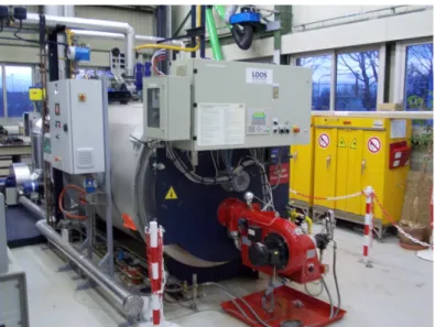
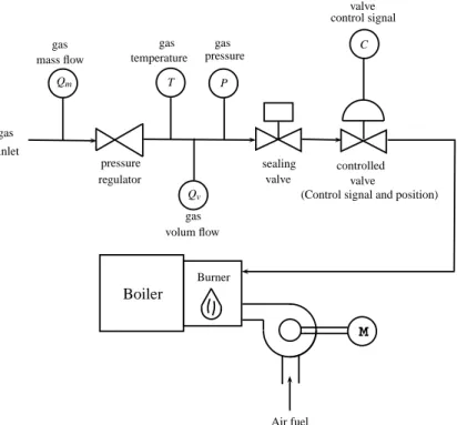
The experimental tests are done on a boiler plant which has a nominal power of 750 kW (see Figure 2). A schematic representation of the boiler installation
and its instrumentation is shown in Figure 3. The mass flow rate of gas is mea-sured before the gas pressure regulator, i.e. in the high pressure part. The gas pressure, temperature and volume flow are measured in the low pressure side. The gas pressure is a manually controlled value but for modeling purposes it is considered as an input. As for the gas temperature, it depends on meteo-rological conditions. In the models that is presented in the following sections, the mass flow is modeled instead of volume flow, because of the dependency of the gas density to the absolute pressure, and thus, to the atmospheric pres-sure. It also depends on the fuel gas composition. The mass flow rate depends directly on the control signal fixed by the operator and sent to the electric valve. This control signal is converted into a position signal depending on the type of used regulating valve. In our case, it is a plug valve.
M Burner Boiler Air fuel T P pressure valve C gas inlet temperature pressure gas gas mass flow gas Qm Qv volum flow gas controlled valve sealing valve
(Control signal and position) regulator
control signal
Fig. 3. Schematic view of the boiler
3.2 Experimental protocol
The experiments realized on this installation consist of a stepwise increase of the electrical control signal C of the modulating gas plug valve. It is fairly easy to collect the valve control signal (which is a value that varies between
0 and 100%). These tests are repeated for different values of pressure p and temperature T of the gas. The pressure is an input data which can be practi-cally controlled by a pressure regulator. It varies between 80 and 200 effective mbar. The gas having a long air routing system, its temperature is thus in-fluenced by weather conditions. The temperature range is from 14 to 33 ◦C.
These experiments are the same ones realized in operation with the aim of calibration of the proposed models.
Figure 4 shows a typical experiment. Figure 5 lists the operating points used in this study.
0 500 1000 20 40 60 80 100 C (%)
Valve position and control signal
0 500 1000 20 40 60 80 Q m (Kg/h)
Gas mass flow
0 500 1000 1.195 1.2 1.205 1.21 Time (s) Absolute P(bar) Gas pressure 0 500 1000 24 25 26 27 Time (s) T (°C) Gas temperature Control signal Position
Fig. 4. Typical test at 200 mbar (effective pressure)
1.05 1.1 1.15 1.2 1.25 10 15 20 25 30 35 p (bars) T (°C)
Fig. 5. Used operating points defined by constant values of the gas pressure and temperature
4 Modeling
Two different modeling approaches are studied: a parametric approach and a non-parametric approach.
One concept of engineering, today, is to model the signals and systems to fa-cilitate the study, analysis and control. This model should be easy to estimate, but at the same time, it must be able to reproduce the main characteristics
of the studied system. To circumvent the complexity of such models, we can use parametric models, which depend on a fixed number of parameters, and whose structure is pre-determined.
Generally, in the second approach which is the non-parametric theory, it is assumed that the number of parameters that describe the observations dis-tribution is an increasing function of the observations dimension, or that the number of parameters is infinite. The non-parametric modeling studies the problems in which the parameterization is not considered as fixed, but there is a choice between multiple parameterization and the objective is to find one that leads to the most efficient procedures.
4.1 Parametric modeling
In this modeling, the primary idea is to consider the mass flow Qm as an
output and C as an exogenous input. However, as can be seen in Figure 6, the pressure p influences the flow value and a simple law only based on the control signal cannot provide a good estimation of the flow. Therefore, we propose an LPV model with one scheduling variable p or two scheduling variables p and
T.
At first, knowing that the pressure has, physically, more influence than the temperature on the gas flow, it is proposed to model the mass flow by taking only the pressure as a scheduling variable. In a second step, we introduce the temperature as a second scheduling variable to see if it has also any influence on the gas flow.
20 30 40 50 60 70 80 90 100 15 20 25 30 35 40 45 50 55 60 65 C (%) Q m (kg/h) 80 mbars 80 mbars 100 mbars 100 mbars 110 mbars 130 mbars 150 mbars 150 mbars 170 mbars 180 mbars 190 mbars 200 mbars
Fig. 6.Flow–control characteristic shape for different gas pressures – measured data
The LPV model, like the other models described in this chapter, is static. The estimated LPV model is obtained by a local approach [8, 23] which con-sists of:
• estimating local models for different operating points of the scheduling variables,
• and calculate the global LPV model by a local models interpolation.
LPV model with one scheduling variable
Local models are estimated at different operating points defined by a con-stant pressure and temperature. With regard to the evolution of the gas flow
Qm depending on the control signal C, the chosen model is presented in the
following polynomial form:
Qm(t) =θ1C(t)2+θ2C(t) +θ3 (1)
The global LPV model as a function of pressure p is determined from the local models. A fixed pressure value is considered throughout the experiment, and is equal to the average of the level corresponding to the highest control signal value. The choice of a fixed value is justified because the pressure varies slightly around a value set by the user via the pressure regulator. It justifies again to consider the pressure as a scheduling variable to fit to different installations. Thus, the parameters θ1,θ2andθ3 variations depending on the pressure are
represented by the following polynomials: θ1= degP ∑ i=0 αi pi θ2= degP ∑ i=0 βi pi θ3= degP ∑ i=0 δipi (2)
where degP represents the polynomial degree of p. The global LPV model becomes: Qm(t) = degP
∑
i=0 αipiC(t)2+ degP∑
i=0 βipiC(t) + degP∑
i=0 δipi (3)LPV model with two scheduling variables
The considered local models are the same as those given by 1. The global LPV model is still obtained by interpolating the evolution of θ1, θ2 and θ3. The
only differences are:
• the average test pressure p is replaced by the instantaneous pressure p(t); • instantaneous temperature T (t) is also taken into account.
The general model is now given by:
Qm= degP ∑ i=0 degT ∑ j=0 αi pi(t) Tj(t)C(t)2 +degP∑ i=0 degT ∑ j=0 βi pi(t) Tj(t)C(t) +degP∑ i=0 degT ∑ j=0 γipi(t) Tj(t) (4)
where degP and degT represent the polynomials degrees of p(t) and T (t). Taking into account the instantaneous measurements including the temper-ature, it is hoped that more accurate estimates than those provided by the first model will be obtained. Each coefficient θ1, θ2 and θ3 is modeled by a
4.2 Non-parametric modeling
Modeling using Gaussian processes is also considered. It is a non parametric approximation method that aims to build an approximation ˆf of the function
Qm= f (C,p,T) from n observations Qmi = f (Ci,pi,Ti),1 ≤ i ≤ n (observations may contain measurement errors), and from a priori about the speed vari-ations of the searched function. To simplify notvari-ations, note xi= (Ci,pi,Ti).
The a priori is expressed assuming that the searched function is the realization of a regular random process, in practice a Gaussian process determined by its mean and covariance function. The mean is here taken equal to zero to reflect the absence of a priori about a possible tendency of f (x). The covariance function is chosen from a set of parameterized covariance functions family (also called kernels) whose parameters are estimated using the maximum likelihood criterion. We considered that the process was stationary and we chose to model its covariance by a Mat´ern covariance [21]. This family of covariance was chosen both for its ability to represent a wide range of processes, because its parameters are easily interpretable, and also because it avoids potential numerical problems.
To express the constraint that the searched function ˆf(x) is close to the n observations, we search among all the Gaussian process realizations, those that explain the observed points: it is the principle of the modeling with Gaussian process that consists of conditioning of the process law with respect to the observations. The conditioned process is actually a new process with a law, including both the a priori (regularity, process variation speed) and the information provided by the observation of the process at some points, can be calculated. This principle is shown in Figure 7 on an example where the variable x is a scalar. 0 0.2 0.4 0.6 0.8 1 −3 −2 −1 0 1 2 3 4 x f(x) obs. yi realizations
Fig. 7. Example of randomly generated realizations from a Gaussian process with Mat´ern covariance of parameters (A = 1,h= 1,ν= 2) conditioned to a set of n = 6 observed values (assumed here free-noise case)
The estimate ˆf(x) commonly used to estimate the function f (x) at one point x is the mean of the process conditioned at this point. The covariance function of the conditioned process enable also to calculate confidence intervals for the function f (x). Figure 8 includes the data of figure 7 (same function f (x), the same abscissa xi and same observed values) and gives the estimate ˆf(x) and
the associated confidence intervals.
0 0.2 0.4 0.6 0.8 1 −3 −2 −1 0 1 2 3 4 x f(x) obs. yi ˆ f(x) Conf. Interv.
Fig. 8. Illustrative example of the Gaussian process modeling – Red dotted lines: function to estimate, red circles: observations, black dotted line: estimation, shaded area: confidence intervals 95 %
5 Experimental results
5.1 Parametric modeling Local models identification
Figure 9 lists the local models, defined by (1), estimated with all 14 avail-able experiments. The parameters have been estimated with a standard least-squares method.
20 30 40 50 60 70 80 90 100 15 20 25 30 35 40 45 50 55 60 65 C (%) Q m (kg/h) 80 mbars 80 mbars 100 mbars 100 mbars 110 mbars 130 mbars 150 mbars 150 mbars 170 mbars 180 mbars 190 mbars 200 mbars 250 mbars 280 mbars
Fig. 9. Local models Qm(t) =θ1C(t)2+θ2C(t) +θ3for different pressure values p
Global models identification
1. LPV model with one scheduling variable
Figures 10 and 11 show the parameters of the different local models based on the operating point of the test. The polynomials, defined by (2), allow a good approximation of the estimated values of the parameters θ1, θ2 andθ3, depending on the pressure as it can be seen in Figure 10. After
several tests, the best results are obtained for degP = 2 for θ1 and θ2,
and degP = 3 forθ3. Figure 11 shows that it is more difficult to define a
mathematical law that fits these points. Initially, it is proposed to use a global LPV model only function of the control signal and the pressure.
60 80 100 120 140 160 180 200 220 −8 −7 −6 −5 −4x 10 −3 θ 1 60 80 100 120 140 160 180 200 220 0.8 1 1.2 1.4 1.6 θ 2 60 80 100 120 140 160 180 200 220 −12 −10 −8 −6
Effective pressure (mbar) θ 3 80 mbars 80 mbars 100 mbars 100 mbars 110 mbars 130 mbars 150 mbars 150 mbars 170 mbars 180 mbars 190 mbars 200 mbars 250 mbars 280 mbars
Fig. 10. Evolution of the local parameters models with respect to the pressure p (markers) and the polynomial models (2) (solid line)
14 16 18 20 22 24 26 28 30 32 34 −8 −6 −4x 10 −3 θ 1 14 16 18 20 22 24 26 28 30 32 34 0.5 1 1.5 θ 2 14 16 18 20 22 24 26 28 30 32 34 −12 −10 −8 −6 T (°C) θ 3
Fig. 11.Evolution of the local parameters models with respect to the temperature
The global LPV model can then be used directly as a soft sensor; for a measured control signal C and a pressure setting, we simply simulate the equation (3) to estimate flow gas. The results of models simulation for an experiment are shown in Figure 12 and compared to the measured data. The maximum relative error (stepwise averaged) is shown in Figure 13 for
all experiment set. Maximum relative error equal to 3.92 % is obtained for a 80 mbar pressure.
0 200 400 600 800 1000 20 30 40 50 60 70 Time (s) Q m (kg/h) Measured flow
Local model flow simulation Global model flow simulation
30 40 50 60 70 80 90 100 0 2 4 6 C (%) Error on Q m (%)
Local model error Global model error Mean error by level
Fig. 12. Local model and one scheduling input global model simulations with 200 mbar experiment data
1 2 3 4 5 6 7 8 9 10 11 12 13 14 0 1 2 3 4 5 6 Experiments
Maximum mean relative error (%)
Fig. 13. Maximum relative errors (stepwise averaged) for 14 tests – LPV model with one scheduling variable
A cross-validation was performed to verify the behavior of the virtual sensor for all experimental conditions potentially faced in the operating phase. The number of experiments is relatively low (14 experiments); we
chose to use a Leave–One–Out approach [16]. It consists to use 13 of the
14tests for identification and one for validation, and repeat this operation so that each test is used as a validation.
The results are shown in Figure 14. The relative errors on the model simulation, estimated using 14 experiments are represented by crosses. The relative errors of the estimated models using 13 experiments and simulated on the validation test are represented by circles. A higher error is noted in validation. Nevertheless, it remains less than 5 % as shown in this figure. 1 2 3 4 5 6 7 8 9 10 11 12 13 14 0 1 2 3 4 5 6 Experiments
Maximum mean relative error (%)
Model on 14 experiments
Model on 13 experiments + validation Mean value
Mean value
Fig. 14. Comparison between the estimated model using 14 experiments and the models from cross-validation – LPV model with one scheduling variable
2. LPV models with two scheduling variables
The global model is now based on the valve control signal C(t) and the in-stantaneous measurements of pressure p(t) and temperature T (t). Figure 15 shows that, at the same pressure, the gas flow at two different temper-atures is not really the same. Remains to be seen if it is really interesting to add a second scheduling variable, and thereby complexify the model.
30 40 50 60 70 80 90 100 15 20 25 30 35 40 C (%) Q m (kg/h) 80 mbars, 23°C 80 mbars, 29°C
Fig. 15.Local models at the same pressure 80 mbar and two different temperatures (23 and 29◦C).
After several tests, the best results are obtained for degP = 2 and degT = 1. The stepwise maximum relative errors in cross-validation are given in Figure 16. The maximum relative error is equal to 3.7 %, i.e. lower than those of the first model. However, it has a higher complexity. Figure 17 presents the simulation of the LPV model obtained for a value of C = 50 % and varying pressures and temperatures. We can note that the influence of pressure on the flow variations is higher than the temperature, which may justify the use of a model taking into account only of the pressure.
1 2 3 4 5 6 7 8 9 10 11 12 13 14 0 1 2 3 4 5 6 Experiments
Maximum mean relative error (%)
Fig. 16. Maximum relative errors (stepwise averaged) in cross-validation – LPV model with two scheduling variables
1.05 1.1 1.15 1.2 1.25 20 25 30 30 35 40 p (bars) T (°C) Q m (kg/h)
Fig. 17. Simulation of the Qm estimated model defined by (4) for a fixed control signal at 50 %
5.2 Non-parametric modeling
The implementation of this method on the 14 experiments realized on the boiler was performed using the Matlab toolbox STK (Small Toolbox for Krig-ing) [2]. As for the other simulations, Figure 18 gives the maximum stepwise relative errors obtained by cross-validation. We can note that the errors are lower than the parametric model errors. In addition, the non-parametric model provides reasonable errors without having to specify structure models.
1 2 3 4 5 6 7 8 9 10 11 12 13 14 0 1 2 3 4 5 6 Experiments
Maximum mean relative error (%)
Fig. 18.Maximum relative errors (stepwise averaged) obtained in cross-validation – non-parametric model
Figure 19 shows the results obtained by cross-validation tests on 4 from the 14 tests. As suggested by the results shown in Figure 18, the predictions are close to the real values. The simulation of the obtained model at variable pressures and temperatures for a 50 % control signal, provides similar results to those presented in Figure 17 . 30 40 50 60 70 80 90 100 10 20 30 40 50 60 70 C (%) Q (kg/h) 280 mbars 80 mbars 100 mbars 150 mbars
Fig. 19.Cross-validation results for Qm= f (C,p,T) models with respect to C – Solid lines: identified polynomials; markers: predictions; dotted lines: associated confidence intervals
5.3 Synthesis
The synthesis of the three different models results is illustrated in Table 2. Although the fact that the parametric model with two scheduling variables and the non-parametric model provide better results in terms of relative er-ror in cross-validation, nevertheless, the parametric LPV with one scheduling variable model still the easiest to implement and calibrate to the real operat-ing conditions. Indeed, it is less complicated to calibrate a system with one variable input than with two variable inputs.
Model Relative error in cross-validation
parametric LPV 1 scheduling variable 5 %
parametric LPV 2 scheduling variables 3.7%
non-parametric 3.8 %
Table 2. Summary table showing the results of the relative errors calculation in cross-validation of the three previous models.
5.4 Soft sensor implementation on the industrial boiler
The LPV model with one scheduling variable was experimented on site owing to its simplicity. The model was directly implemented on the PLC with C#
programming language. The pressure setpoint has been tuned and fixed to the value read on the manometer during the pressure regulator setting. Figure 20 shows the flow measurement with the soft sensor. As we can see, the results are acceptable with a maximum mean relative error of 3.5 % for the LPV model with one scheduling variable.
0 200 400 600 800 25 30 35 40 45 50 55 60 65 Time (sec) Q m (kg/h)
Validation test at 210 mbars
measured mass flow LPV 1 scheduling var.
Fig. 20.Experimental simulation of the soft sensor based on the LPV model with one scheduling variable
6 Conclusion
This chapter reviewed the current technologies intended to flow and power measurements from a material and financial point of view. We have seen that measuring is the key for improving Energy Efficiency in the manufacturing sector, hence the necessity to look for smart low cost sensors.
In particular, the modeling of an industrial boiler was investigated towards a consumed gas flow measurement. Three static models were estimated: two LPV parametric models and a non-parametric model. A cross-validation showed that the simulation of these models gives a flow measurement er-ror lower than 5 %. This value corresponds to the fixed objectives of low-cost sensors implementation that allow consumption monitoring and detection of possibles drifts.
Models degraded uses should also be considered. While the online temperature measurement could be considered low-cost, this is not the case of the pressure. But, in practice, the boiler engineer tunes the pressure with the pressure regulator and measures it with manometer.
Finally, the genericity of models to different installations and other kinds of valves, should be studied. It is then necessary to define a model parameters calibration methodology which is the least intrusive. To do this, a grey box model is being tested. Its purpose is to find generic models for all sorts of valves existing in industry for all types of boilers, with different pipe dimensions. There exists a valve opening law: Qgas= f (C%), Qgasbeing the gas flow, which
should be different from a valve to another. The equation Qgas= Kv√p1− p2,
with p1 and p2 the pressures before and after the valve, and Kv the flow
coefficient, needs also to be considered. The objective here is to estimate
Qgas froms these two expressions, taking into account the valve manufacturer
datasheet and the pipe dimensions.
Acknowledgment
This work has been supported by the French Research National Agency (ANR) through Efficacit´e ´energ´etique et r´eduction des ´emissions de CO2 dans les
syst`emes industrielsprogram (project CHIC n◦ANR-10-EESI-02).
References
1. Arkoun O., Estimation non param´etrique pour les mod`eles autor´egressifs, The-sis, University of Rouen, France, 2009.
2. Bect J. and Vasquez E., A small (Matlab/GNU Octave) Toolbox for Kriging, (http://sourceforge.net/projects/kriging/), Supelec, 2011.
3. Bogaerts P. and Vande Wouwer A., Software sensors for bioprocesses, ISA Trans-actions 42, 547-558, 2003.
4. Bourkeb M., Ondel O., Joubert C., Morel L., Scorretti R., M´ethodes num´eriques pour la mesure de courant dans un syst`eme polyphas´e, Num´elec 2012. European conference on numerical methods and electromagnetism, 3-5 July, 2012, Mar-seille, France.
5. Cecil D. and Kozlowska M., Software sensors are a real alternative to true sen-sors. Environmental Modelling & Software 25, 622-625, 2010.
6. Ch´eruy A., Software sensors in bioprocess engineering. Journal of Biotechnology 52, 193-199, 1997.
7. Dochain D., State and parameter estimation in chemical and biochemical pro-cesses: a tutorial. J. Proc. Control 13, 801-818, 2003.
8. Dos Santos P. L., Perdico`ulis T. A., Novara C., Ramos J. and Rivera D., Linear Parameter-Varying System Identification: new developments and trends Ad-vanced Series in Electrical and Computer Engineering. World Scientific, 2011. 9. Etien E., Modeling and simulation of soft sensor design for real-time speed
estimation, measurement and control of induction motor, ISA Transactions, Vol. 52, pp. 358–364, 2013.
10. Gever M., Toward a joint design of identification and control ?, Birkh¨auser– Boston, H.L. Trentelman and J.C. Willems, 1993.
11. Grau A. et al, Low cost power and flow rates measurements for manufacturing plants, 16th international congress of metrology, Paris, France, October 2013. 12. Grospeaud O., Contribution `a l’identification en boucle ferm´ee par erreur de
sortie, Thesis, University of Poitiers, Poitiers, France, 2000.
13. Hadid B., Etien E., Ouvrard R., Poinot T., Le Brusquet L., Grau A., Schmitt G., Soft Sensor Design for Power Measurement and Diagnosis in Electrical Fur-nace: a Parametric Estimation Approach, 39th Annual Conference of the IEEE Industrial Electronics Society IECON, Vienna, Austria, November 2013. 14. Hadid B., Ouvrard R., Le Brusquet L., Etien E., Poinot T., Sicard F., Modeling
for gas flow measurement consumed by a boiler. Towards a low-cost sensor for energy efficiency, Seventh International Conference on Sensing Technology ICST, Massey University, Wellington, New Zealand, 2013.
15. James S.C., Legge R.L. and Budman H., On-line estimation in bioreactors: a review. Rev. Chem. Eng. 16 (4), 311-340, 2000.
16. Kohavi R., A study of cross-validation and bootstrap for accuracy estimation and model selection. Proceedings of the Fourteenth International Joint Confer-ence on Artificial IntelligConfer-ence 2 (12), 1137-1143, 1995.
17. Le Mouel A. et al, Fostering Energy Efficiency in manufacturing plants through economical breakthroughs in power and flow rate measurement, ECEEE Sum-mer Study on Industry, Arnhem, Germany, 2012.
18. Ljung L., System identification. Theory for the user, 2nd edition, 1999. 19. Queinnec I. and Sp´erandio M., Simultaneous estimation of
nitrifica-tion/denitrification kinetics and influent nitrogen load using orp and do dy-namics. ECC, Cambridge, UK, 2003.
20. Poinot T., Contribution `a l’identification des syst`emes par la m´ethode de sur-param´etrisation en traitement des eaux, Thesis, Universit´e de Poitiers, France, 1996.
21. Rasmussen C.E. and Williams K.I., Gaussian Processes for Machine Learning. The MIT Press, 2006.
22. Sotomayor O. A. Z., Won Park S. and Garcia C., Software sensor for on-line es-timation of the microbial activity in activated sludge systems. ISA Transactions 41, 127-143, 2002.
23. T´oth R., Identification and Modeling of Linear Parameter-Varying Systems Springer Verlag. Lecture Notes in Control and Information Sciences 403, 2010. 24. Van Donkelaar E.T. and P.M.J. Van den Hof, Analysis of closed-loop iden-tification with a tailor-made parametrization, European Control Conference, Brussels, Belgium, Vol. 4, 1997.