HAL Id: hal-02960278
https://hal.archives-ouvertes.fr/hal-02960278
Preprint submitted on 7 Oct 2020
HAL is a multi-disciplinary open access
archive for the deposit and dissemination of
sci-entific research documents, whether they are
pub-lished or not. The documents may come from
teaching and research institutions in France or
abroad, or from public or private research centers.
L’archive ouverte pluridisciplinaire HAL, est
destinée au dépôt et à la diffusion de documents
scientifiques de niveau recherche, publiés ou non,
émanant des établissements d’enseignement et de
recherche français ou étrangers, des laboratoires
publics ou privés.
ejecta of Cassiopeia A using a component separation
method in X-rays
A Picquenot, F Acero, T Holland-Ashford, L Lopez, J Bobin
To cite this version:
A Picquenot, F Acero, T Holland-Ashford, L Lopez, J Bobin. Three-dimensional morphological
asymmetries in the ejecta of Cassiopeia A using a component separation method in X-rays. 2020.
�hal-02960278�
Wednesday 7thOctober, 2020
Three-dimensional morphological asymmetries in the ejecta of
Cassiopeia A using a component separation method in X-rays
A. Picquenot
1, F. Acero
1, T. Holland-Ashford
2,3, L. A. Lopez
2,3, and J. Bobin
11AIM, CEA, CNRS, Université Paris-Saclay, Université Paris Diderot, Sorbonne Paris Cité, F-91191 Gif-sur-Yvette, France
2Department of Astronomy, The Ohio State University, 140 W. 18th Ave., Columbus, OH 43210, USA
3Center for Cosmology and AstroParticle Physics, The Ohio State University, 191 W. Woodruff Ave., Columbus, OH 43210, USA
Wednesday 7thOctober, 2020
ABSTRACT
Recent simulations have shown asymmetries in the ejecta distribution of supernova remnants can still reflect asymmetries from the initial supernova explosion. Thus, their study provides a great mean to test and constrain model predictions in relation to the distribu-tion of heavy elements or the neutron star kicks, both being key subjects for a better understanding of the explosion mechanisms in core-collapse supernovae.
The use of a novel blind source separation method applied to the megasecond X-ray observations of the well-known Cassiopeia A supernova remnant revealed maps of the distribution of the ejecta endowed with an unprecedented level of detail and clearly separated from continuum emission. Our method also provides a three-dimensional view of the ejecta by disentangling the red- and blue-shifted spectral components and associated images of the Si, S, Ar, Ca and Fe, giving insights on the morphology of the ejecta distribution in Cassiopeia A. These mappings allow us to investigate thoroughly the asymmetries in the heavy elements distribution and probe simulation predictions about the neutron star kicks and the relative asymmetries between the different elements.
We find in our study that most of the ejecta X-ray flux stems from the red-shifted component suggesting an asymmetry in the explosion. In addition, the red-shifted ejecta can physically be described as a broad, relatively symmetric plume, whereas the blue-shifted ejecta is more similar to a dense knot. The neutron star also moves directly opposite to the red-shifted parts of the ejecta similar to what is seen with44Ti. Regarding the morphological asymmetries, it appears that heavier elements have more asymmetrical distributions,
which confirms predictions made by simulations. This study is a showcase of the capacities of new analysis methods to revisit archival observations to fully exploit their scientific content.
1. Introduction
Cassiopeia A (hereafter, Cas A) is among the most studied as-tronomical objects in X-rays and is arguably the best-studied supernova remnant (SNR). Investigation of the distribution of metals on sub-parsec scales is possible because it is the youngest core-collapse (CC) SNR in the Milky Way (about 340 years old ; Thorstensen et al. 2001), its X-ray emission is dominated by the ejecta metals (Hwang & Laming 2012), and it is relatively close (3.4 kpc ; Fesen et al. 2006). Cas A benefits from extensive ob-servations (about 3 Ms in total by Chandra), making it an ideal laboratory to probe simulation predictions regarding the distri-bution of ejecta metals.
In the last few years, 3D simulations of CC SNe have be-gun to produce testable predictions of supernovae explosion and compact object properties in models using the neutrino-driven mechanism (see reviews by Janka et al. 2016; Müller 2016). In particular, explosion-generated ejecta asymmetries (Wong-wathanarat et al. 2013; Summa et al. 2018; Janka 2017) and neu-tron star (NS) kick velocities (Thorstensen et al. 2001) appear to be key elements in CC SNe simulations that Cas A’s data can constrain. Although it is challenging to disentangle the asymme-tries produced by the surrounding medium from those inherent to the explosion, Orlando et al. (2016) has explored the evolu-tion of the asymmetries in Cas A using simulaevolu-tions beginning from the immediate aftermath of the SN and including the 3D interactions of the remnant with the interstellar medium. Simi-lar simulations presenting the evolution of a Type Ia SNR over a period spanning from one year after the explosion to several
centuries afterwards have been made by Ferrand et al. (2019), showing that asymmetries present in the original SN can still be observed after centuries. The same may go with the CC SNR Cas A, and a better knowledge of its 3D morphology could lead to a better understanding of the explosion mechanisms by pro-viding a way to test the simulations.
An accurate mapping of the different elements’ distribution, the quantification of their relative asymmetries, and their rela-tion to the NS morela-tion would, for example, allow us to probe the simulation predictions that heavier elements are ejected more asymmetrically and more directly opposed to the NS motion than lighter elements (Wongwathanarat et al. 2013; Janka 2017; Gess-ner & Janka 2018; Müller et al. 2019). On this topic, this paper can be seen as a follow-up to Holland-Ashford et al. (2020), the first study to quantitatively compare the relative asymmetries of different elements within Cas A, but that suffered from difficulty separating and limiting contamination in the elements’ distribu-tion. Moreover, in that analysis, the separation of the blue- and red-shifted parts in these distributions was not possible.
Here, we intend to fix these issues by using a new method to retrieve accurate maps for each element’s distribution, allow-ing us to investigate further their individual and relative physical properties. This method, based on the General Morphological Components Analysis (GMCA, see Bobin et al. 2015), a blind source separation (BSS) algorithm that was introduced for X-ray observations by Picquenot, A. et al. (2019). It can disentangle both spectrally- and spatially-mixed components from an X-ray data cube of the form (x, y, E) with a precision unprecedented in
this field. The new images thus obtained suffer from less contam-ination by other components, including the synchrotron emis-sion. It also offers the opportunity to separate the blue- and red-shifted parts of the elements’ distribution, thereby facilitating a 3D mapping of the X-ray emitting metals and a comparison of their relative asymmetries. Specifically, the GMCA is able to dis-entangle detailed maps of a red- and a blue-shifted parts in the distributions of Si, S, Ca, Ar and Fe, thus providing new and crucial information about the 3D morphology of Cas A.
This paper is structured as follows. In Section 2, we will de-scribe the nature of the data we use (Section 2.1), our extraction method (Section 2.2), our way to quantify the asymmetries (Sec-tion 2.3), and our method to retrieve error bars (Sec(Sec-tion 2.4). In Section 2, we will present the images resulting from the applica-tion of our extracapplica-tion method (Secapplica-tions 3.1 and 3.2) and the find-ings obtained when we quantify their asymmetries (Section ??), will discuss the interpretation of the retrieved images as blue- or red-shifted by looking at their associated spectra (Section 3.3), and will present the results of a spectral analysis on these same spectra (Section 3.4). Lastly, we will discuss in Section 4 the physical information we can infer from our results. Section 4.1 will be dedicated to the interpretation of the spatial asymmetries of each line emission, while Sections 4.2 and 4.3 will focus re-spectively on the mean direction of each line’s emission and on the NS velocity. A comparison with the NuSTAR data of44Ti will finally be presented in Section 4.4.
2. Method
2.1. Nature of the data
Spectro-imaging instruments, such as those aboard the current generation of X-ray satellites XMM-Newton and Chandra, pro-vide data comprised of spatial and spectral information: the de-tectors record the position (x, y) and energy E event by event, thereby producing a data cube with two spatial dimensions and one spectral dimension. For our study, we used Chandra obser-vations of the Cas A SNR, which was observed with the ACIS-S instrument in 2004 for a total of 980 ks (ObsID : 4634, 4635, 4636, 4637, 4638, 4639, 5196, 5319, 5320; Hwang et al. 2004). We used only the 2004 dataset to avoid the need to correct for proper motion across epochs. The event lists from all observa-tions were merged in a single data cube. The spatial (of 200) and spectral binning (of 14.6 eV) were adapted so as to obtain a suf-ficient number of counts in each cube element. No background subtraction or vignetting correction has been applied to the data.
2.2. Image Extraction
In order to study asymmetries in the ejecta metals in Cas A, a good mapping of their spatial distribution is needed. How-ever, extracting the spatial distribution of each element is not a straightforward process as multiple components, such as the shocked ejecta and the synchrotron emission, are overlapping, sometimes with a high contrast factor. Picquenot, A. et al. (2019) introduced a method that was able to disentangle both morphologically- and spectrally-accurate components from a (x, y, E) X-ray data cube. This method was based on the GMCA, a BSS algorithm first introduced in Bobin et al. (2015).
The main concept of GMCA is to take into account the morphological particularities of each component in the wavelet domain to disentangle them, without any prior instrumental or physical information. Apart from the (x, y, E) data cube, the only input needed is the number n of components to retrieve, which
is user-defined. The outputs are then a set of n images associated with n spectra. Each couple image-spectrum represents a compo-nent: the algorithm makes the assumption that every component can be described as the product of an image with a spectrum. Thus, the retrieved components are approximations of the actual components with the same spectrum on each point of the im-age. Nevertheless, Picquenot, A. et al. (2019) showed that when tested on Cas A-like toy models, the GMCA was able to ex-tract morphologically and spectrally accurate results. The tested spectral toy models included power-laws, thermal plasmas, and Gaussian lines. In particular, in one of these toy models, the method was able to separate three components: two nearby par-tially overlapping Gaussian emission lines and power-law emis-sion. The energy centroids of both Gaussians were accurately retrieved, despite their closeness. Such a disentangling of mixed components with similar neighbouring spectra cannot be ob-tained through line-interpolation, and fitting of a two-Gaussian model region by region is often time consuming, producing im-ages contaminated by other components with unstable fitting re-sults.
In the same paper, the first applications on real data of Cas A were promising, in particular concerning asymmetries in the el-ements’ distribution. For Si, S, Ar, Fe and Ca, the GMCA was able to retrieve two maps associated with spectra slightly blue-or red-shifted from their theblue-oretical position. The existence of blue- or red-shifted parts in these elements’ distribution was pre-viously known, and the Fe maps from Picquenot, A. et al. (2019) were consistent with prior works but endowed with more details (see Willingale et al. 2002a; DeLaney et al. 2010). Thus, they constitute a great basis for an extensive study of the asymme-tries in the elements’ distribution in Cas A.
In this paper, we will use a more recent version of the GMCA, the pGMCA, that was developed to take into account data of a Poissonian nature (Bobin et al., submitted). In the precedent version of the algorithm, the noise was supposed to be Gaussian. Even with that biased assumption, the results were proven to be reliable. However, a proper treatment of the noise is still relevant : it increases the consistency of the spectral mor-phologies of the retrieved components and makes the algorithm able to disentangle components with a fainter contrast.
The mathematical formalism is highly similar to that of the GMCA, presented in Picquenot, A. et al. (2019). The funda-mental difference is that instead of a linear representation, the pGMCA uses the notion of Poisson-likelihood of a given sum of components to be the origin of a certain observation. The prob-lem solved by the algorithm is thus of the same kind, with mainly a change in the nature of the norm to minimize. For a more pre-cise description of this new method, see Bobin et al., submitted1. The use of the pGMCA is also highly similar to that of the GMCA. One notable difference is that the pGMCA is more sen-sitive to the initial conditions, so it needs a first guess for conver-gence purposes. The analysis therefore consists of two steps : a first guess obtained with the GMCA and a refinement step using the Poissonian version pGMCA.
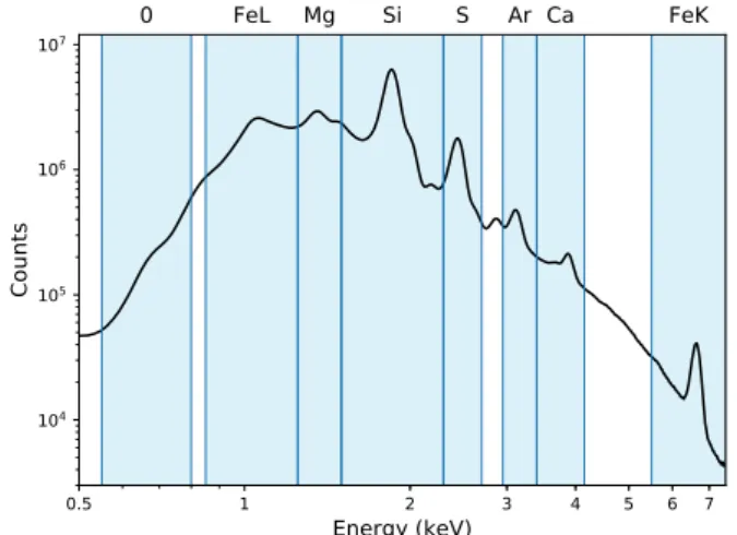
The aforementioned workflow was applied to the Cas A Chandra observations by creating data cubes for each energy band shown in Fig. 1. These energy bands were chosen to be large enough to have the leverage to allow the synchrotron con-tinuum to be correctly retrieved and to be narrow enough to avoid contamination by other line emissions. The pGMCA be-ing a fast-runnbe-ing algorithm, the final energy bands were chosen after tests to find the best candidates for both criteria. For each
0.5 1 2 3 4 5 6 7
Energy (keV)
104 105 106 107Counts
0
FeL Mg
Si
S Ar Ca
FeK
Fig. 1: Spectrum of Cas A obtained from the combination of the deep Chandra 2004 observations. The source separation algo-rithm was applied in each individual energy band represented by the shaded regions.
band, the initial number of components n was 3 : the synchrotron emission and the blue- and red-shifted parts of the line emission. We then tested using 4 and 5 components to ensure extra com-ponents were not merged into our comcom-ponents of interest. We also tested with 2 components to verify our assumption on the presence of blue- and red-shifted parts was not imposing the ap-parition of a spurious component. For each emission line, we then chose n as the best candidate to retrieve the most seemingly meaningful components without spurious images.
For each analysis, the algorithm was able to retrieve a com-ponent that we identify as the synchrotron emission (a power-law spectrum and filamentary spatial distribution, not shown here) and multiple additional thermal components with strong line features. We were able to identify two associated images with shifted spectra from the theoretical emission line energy for all these line features except O, Mg, and Fe L.
2.3. Quantification of asymmetries
We use the power-ratio method (PRM) to quantitatively ana-lyze and compare the asymmetries of the images extracted by pGMCA. This method was developed by Buote & Tsai (1995) and previously employed for use on SNRs (Lopez et al. 2009; Lopez et al. 2009, 2011). It consists of calculating multipole moments in a circular aperture positioned on the centroid of the image, with a radius that encloses the whole SNR. Powers of the multipole expansion Pmare then obtained by integrating the mth term over the circle. To normalize the powers with respect to flux, they are divided by P0, thus forming the power ratios Pm/P0. For a more detailed description of the method, see Lopez et al. (2009).
P2/P0and P3/P0convey complementary information about the asymmetries in an image. The first term is the quadrupole power-ratio and quantifies the ellipticity/elongation of an ex-tended source, while the second term is the octupole power-ratio and is a measure of mirror asymmetry. Hence, both are to be compared simultaneously to ascertain the asymmetries in di ffer-ent images.
Here, as we want to compare asymmetries in the blue- and red-shifted part of the elements’ distribution, the method is
slightly modified. In a first step, we calculate the P2/P0 and P3/P0ratios of each element’s total distribution by using the sum of the blue- and red-shifted maps as an image. Its centroid is then an approximation of the center-of-emission of the considered element. Then, we calculate the power ratios of the blue- and red-shifted images separately using the same center-of-emission. Ultimately, we normalize the power ratios thus obtained by the power ratios of the total element’s distribution :
Pi/P0 (shifted/ total)= Pi/P0 (red or blue image) Pi/P0 (total image)
(1)
where i= 2 or 3 and Pi/P0(red or blue image) is calculated us-ing the centroid of the total image. That way, we can compare the relative asymmetries of the blue- and red-shifted parts of di ffer-ent elemffer-ents, without the comparison being biased by the origi-nal asymmetries of the whole distribution.
2.4. Error bars
As explained in Picquenot, A. et al. (2019), error bars can be obtained by applying this method on every image retrieved by the GMCA applied on a block bootstrap resampling. However, as was shown in that paper, this method introduces a bias in the results of the GMCA. We show in Appendix B that the block bootstrap method modifies the Poissonian nature of the data, thus impacting the results of the algorithm. Since the pGMCA is more dependent than GMCA on the initial conditions, the bias in the outputs is even greater with this newer version of the al-gorithm (see Fig. B.3). For that reason, we developed a new re-sampling method we named "constrained bootstrap", presented in Appendix B.4.
Thus, we applied pGMCA on a hundred resamplings ob-tained thanks to the constrained bootstrap for each emission line and plotted the different spectra we retrieved around the ones obtained on real data. As stated in Appendix B.4, the spread be-tween the resamplings has no physical significance but helps in evaluating the robustness of the algorithm around a given set of original conditions. The blue-shifted part of the Ca line emis-sion, a very weak component, was not retrieved for every re-sampling. In this case, we created more resamplings in order to obtain a hundred correctly retrieved components. The faintest components are the ones with the largest relative error bars, as can be seen in Fig. 3 and Fig. 8, highlighting the difficulty for the algorithm to retrieve them in a consistent way on a hundred slightly different resamplings.
To obtain the error bars for the PRM plot of the asymme-tries, we applied the PRM to the hundred images retrieved by the pGMCA on the resamplings. Then, in each direction we plotted error bars representing the interval between the 10thand the 90th percentile and crossing at the median. We also plotted the PRM applied on real data. Although our new constrained bootstrap method ensures the Poissonian nature of the data to be preserved in the resampled data sets, we see that the results of the pGMCA on real data are sometimes not in the 10th-90thpercentile zone, thus suggesting there may still be some biases. It happens mostly with the weakest components, showing once more the difficulty for the pGMCA to retrieve them consistently out of different data sets presenting slightly different initial conditions. How-ever, even when the results on real data are not exactly in the 10th-90thpercentile zone, the adequation between the results on real and resampled data sets is still good, and the relative
posi-Red-shifted part Blue-shifted part Si 0.60 0.40 S 0.61 0.39 Ar 0.63 0.37 Ca 0.80 0.20 Fe-K 0.70 0.30
Table 1: Fractions of the counts in the total image that belong to the red-shifted or the blue-shifted parts, for each line.
tioning for each line is the same, whether we consider the results on the original data or on the resampled data sets.
3. Results
3.1. Images retrieved by pGMCA
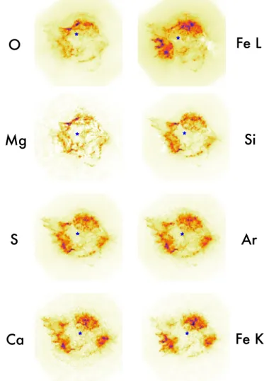
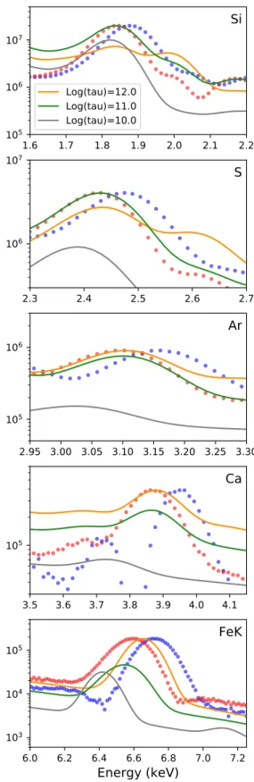
By applying the pGMCA algorithm on the energy bands sur-rounding the eight emission lines shown in Fig. 1, we were able to retrieve maps of their spatial distribution associated with spec-tra, successfully disentangling them from the synchrotron emis-sion or other unwanted components. The O, Mg, and Fe L lines were only retrieved as single features, each associated with a spectrum, whereas Si, S, Ar, Ca and Fe-K were retrieved as two different images associated with spectra that we interpret as be-ing the same emission lines slightly red- or blue-shifted. Fig. 2 shows the total images for all eight line emissions, obtained by summing the blue- and red-shifted parts when necessary. It also indicates the centroid of each image that is adopted in the PRM. Fig. 3 shows the red- and blue-shifted parts of five line emissions, together with their associated spectra, while Fig. 8 presents the images of O, Mg, and Fe L together with their re-spective spectra.
3.2. Discussion on the retrieved images
The fact that our algorithm fails to separate a blue-shifted from a red-shifted part in the O, Mg, and Fe L images is not surprising. At 1 keV, we infer that a radial speed of 4000 km s−1would lead to a∆E of about 13 eV, which is below the spectral bin size of our data. We see in Fig. 2 that while the O and the Mg images are highly similar, they are both noticeably different from the images of the other line emissions. Both the O and Mg images exhibit similar morphology to the optical images of O ii and O iii from Hubble (Fesen et al. 2001; Patnaude & Fesen 2014). The intermediate mass elements share interesting properties : their spatial distributions appears similar in Fig. 2, and the division into a red- and a blue-shifted parts (as found by the pGMCA) allows us to investigate their three-dimensional morphology. We also notice that the maps of Si and Ar are similar to the Arii in infrared (DeLaney et al. 2010).
We quantify the asymmetries in the images using the PRM method described in Sect. 2.3. Fig. 4 presents the quadrupole power-ratios P2/P0 versus the octupole power-ratios P3/P0 of the total images from Fig. 2. Fig. 5 shows the quadrupole power-ratios versus the octupole power-ratios of the red- and blue-shifted images presented in Fig. 5 normalized with the quadrupole and octupole power-ratios of the total images (Fig. 2) as defined in Eq. 2.3.
Si
Fe K
Mg
Fe L
Ar
Ca
S
O
Fig. 2: Total images of the different line emissions’ spatial struc-ture as retrieved by the pGMCA. The blue dot represents the image centroid adopted in the PRM analysis. The color-scale is in square root.
3.3. Discussion on the retrieved spectra
As stated before, it is the spectra retrieved together with the aforementioned images that allow us to identify them as "blue-" or "red-shifted" components. Here we will expand on our rea-sons to support these assertions.
The spectra in Fig. 3 are superimposed with the theoretical positions of the main emission lines in the energy range. In the case of Si, the retrieved features are shifted to the left or right of the rest-energy positions of the theoretical Si xiii and Si xiv lines. Appendix A shows that this shifting is not primarily due to an ionization effect, as the ratio Si xiii/Si xiv is roughly equal in both cases. The same goes for S, where two lines corresponding to S xv and S xvi are shifted together while keeping a similar ratio.
A word on the Ca blue-shifted emission : this component is very weak and in a region where there is a lot of spatial overlap, making it difficult for the algorithm to retrieve. For that reason, the retrieved spectrum has a poorer quality than the others, and it was imperfectly found on some of our constrained bootstrap resamplings. Consequently, we were compelled to run the algo-rithm on more than a hundred resamplings and to select the ac-curate ones to obtain a significant envelop around the spectrum obtained on the original data.
Red-shift
Blue-shift
Si
S
Ar
Ca
Fe K
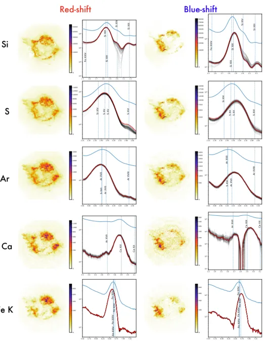
Fig. 3: Red- and blue-shifted parts of the Si, S, Ar, Ca and Fe line emission spatial distribution and their associated spectrum as found by pGMCA. The spectra in red correspond to the application of the algorithm on real data, while the dotted gray spectra correspond to the application on a hundred constrained bootstrap resamplings. The dotted lines represent the energy of the brightest emission lines for a non-equilibrium ionization plasma at a temperature of 1.5 keV and ionization timescale of log(τ)= 11.3 cm−3s produced using the AtomDB (Foster et al. 2012). These parameters are the mean value of the distribution shown in Fig.2 of Hwang & Laming (2012).
Line Erest Ered Eblue ∆V Vred Vblue keV keV keV km/s km/s km/s Si xiii 1.8650 1.860 1.896 5787 804 4983 Si xiii∗ 1.8730 1.860 1.896 5762 2081 3681 S xv 2.4606 2.439 2.489 6092 2632 3460 Ar xvii 3.1396 3.110 3.180 6684 2826 3858 Ca xix 3.9024 3.880 3.967 6684 1721 4963 Fe complex 6.6605 6.599 6.726 5716 2768 2948 Table 2: Spectral fitting on individual lines and resulting veloc-ities. Si and Fe line rest energy are taken from DeLaney et al. (2010). The Si XIII∗uses a different rest energy, the one needed to match the ACIS and HETG Si velocities discussed in DeLaney et al. (2010), to illustrate possible ACIS calibration issues.
3.4. Spectral analysis
Using the spectral components retrieved for each data subset shown in Fig. 3, we carried out a spectral fitting assuming a residual continuum plus line emission in XSPEC (power-law+ gaussmodel). In this analysis, the errors for each spectral data point are derived from the constraint bootstrap method presented in Appendix B. This constrained bootstrap eliminates a bias in-troduced by classical bootstrap methods and that is critical to pGMCA, but underestimates the true statistical error. Therefore no statistical errors on the line centroids are listed in Table 2 as, in addition, systematic errors associated with ACIS energy cali-bration are likely to be the dominant source of uncertainty.
Fe K Ca O Fe L Ar S Mg Si Mirror Asymmetry El li p ti c a l A s y m m e tr y
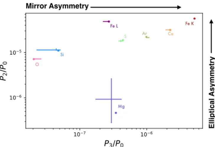
Fig. 4: The quadrupole power-ratios P2/P0 versus the octupole power-ratios P3/P0of the total images of the different line emis-sions shown in Fig. 2. The dots represent the values measured for the pGMCA images obtained from the real data, and the crosses the 10th and 90th percentiles obtained with pGMCA on a hun-dred constrained bootstrap resamplings, with the center of the cross being the median.
Si S Ar Ca Fe K Si S Ar Ca Fe K Mirror Asymmetry El li p ti c a l A s y m m e tr y
Fig. 5: The quadrupole power-ratios P2/P0 versus the octupole power-ratios P3/P0 of the red- and blue-shifted images of the different line emissions shown in Fig. 3, normalized with the quadrupole and octupole power-ratios of the total images. The dots and errorbar as obtained in the same way as in Fig. 4
The resulting line centroid and equivalent velocity shifts are shown in Table 2. To transform the shift in energy into a velocity shift, a rest energy is needed. The ACIS CCD spectral resolu-tion does not resolve the line complex and cannot easily disen-tangle velocity and ionization effects. However given the range of ionization state observed in Cas A (with ionization ages of tau ∼1011− 1012cm−3s, see Fig. 2 of Hwang & Laming 2012), there is little effect of ionization on the dominant line for Si, S, Ar and Ca, as discussed in more details in Appendix A. The line rest energy was chosen as the brightest line for a non-equilibrium ionization plasma with a temperature of 1.5 keV temperature and log(τ)= 11.3 cm−3s, the mean values from Fig. 2 of Hwang & Laming (2012).
For the specific case of the Si xiii line, a very large asym-metry in the red/blue-shifted velocities is observed. This could
Si S Ar Ca Fe K Si S Ar Ca Fe K Center of explosion 20 arcsec Neutron star Ti 44
Fig. 6: Centroids of the blue- and red-shifted parts of each line emission and their distance from the center of explosion of Cas A. For reference, we added the direction of motion of the 44Ti in black, as shown in Fig. 13 of Grefenstette et al. (2017). Only the direction is relevant, as the norm of this specific vector is arbitrary.
Si
S
Ar
Ca
Fe K
80 90 100 110 120 130 140Angle (degrees)
Fig. 7: Angles between the directions of the red- and blue-shifted centers of emission toward the center of explosion for each ele-ment.
be due to possible energy calibration issues near the Si line as shown by DeLaney et al. (2010) in a comparison of ACIS and HETG line centroid, resulting in a systematic blue-shift effect in ACIS data. The Si xiii∗ line in Table 2 uses a corrected rest line energy to illustrate systematic uncertainties associated with calibration issues.
For the Fe-K complex of lines, we rely on the analysis of DeLaney et al. (2010) who derived an average rest line energy of 6.6605 keV (1.8615 Å) by fitting a spherical expansion model to their 3D ejecta model. Note that with this spectral analysis, what we measure here is the radial velocity that is flux weighted over the entire image of the associated component. Therefore we are not probing the velocity at small angular scale but the bulk velocity of the entire component.
With the caveats listed above, we notice an asymmetry in the velocities where ejecta seem to have a higher velocity towards us (blue-shifted) than away from us, even in the case of Si xiii after calibration corrections.
O
Mg
Fe L
Fig. 8: Images of the O, Mg, and Fe L line emission spatial struc-tures and their associated spectrum as found by pGMCA. The spectra in red correspond to the application of the algorithm on real data, while the dotted gray spectra correspond to the appli-cation on a hundred constrained bootstrap resamplings.
The large uncertainties associated with the energy calibra-tion and the choice of rest energy has little impact on the delta between the red- and blue shifted centroids and hence on the∆V. We note that all elements show a consistent∆V of ∼6000 km s−1.
4. Physical Interpretation
4.1. Quantification of ejecta asymmetries
Fig. 4 shows that the distribution of heavier elements is generally more elliptical and more mirror asymmetric than that of lighter elements in Cas A : O, Si, S, Ar, Ca, and Fe emission all exhibit successively higher levels of both measures of asymmetry. This result is consistent with the recent observational study of Cas A by Holland-Ashford et al. (2020), suggesting that the pGMCA method accurately extracts information from X-ray data cubes without the complicated and time-consuming step of extracting spectra from hundreds or thousands of small regions and analyz-ing them individually.
Similar to the results of Holland-Ashford et al. (2020) and Hwang & Laming (2012), Mg emission does not follow the ex-act same trend as the other elements : it has roughly an order of magnitude lower elliptical asymmetry (P2/P0) than the other el-ements. In contrast to Holland-Ashford et al. (2020) and Hwang
& Laming (2012), our Mg image (as shown in Fig. 8) presents a morphology highly different from that of the Fe L ; we believe that the pGMCA was able to retrieve the Mg spatial distribution with little continuum or Fe contamination.
Fig. 5 presents the relative ellipticity/elongation and mirror asymmetries of the blue- and red-shifted ejecta emission com-pared to the total ejecta images (Fig. 2). A value of “1” in-dicates that the velocity-shifted ejecta has equivalent levels of asymmetry as the full bandpass emission. In the cases where we can clearly disentangle the red- and blue-shifted emission (i.e. Si, S, Ar, Ca, and Fe-K, described in previous paragraphs), we see that the red-shifted ejecta emission is less asymmetric than the blue-shifted emission. This holds true both for elliptical asymmetry P2/P0and mirror asymmetry P3/P0. Thus, we could physically describe the red-shifted ejecta distribution as a broad, relatively symmetric plume, whereas the blue-shifted ejecta is concentrated into dense knots. This interpretation matches with the observation that most of the X-ray emission is from the red-shifted ejecta, as we can also see in the flux ratios shown in Table 1 and in the images of Fig. 3, suggesting that there was more mass ejected away from the observer, neutron star, and blue-shifted ejecta knot. We note that there is not a direct corre-lation between ejecta mass and X-ray emission due to the posi-tion of the reverse shock, the plasma temperature and ionizaposi-tion timescale, but the indication that most of the X-ray emission is red-shifted is consistent with our knowledge of the44Ti distribu-tion (see Sect. 4.4 for a more detailed discussion).
Furthermore, in all cases, the red-shifted ejecta emission is more circularly symmetric than the total images, and the blue-shifted ejecta is more elliptical/elongated than the total images. Moreover, the red-shifted ejecta is more mirror symmetric than the shifted ejecta, though both the red-shifted and blue-shifted Si are more mirror asymmetric than the total image. The latter result may suggest that the red-shifted and blue-shifted Si images’ asymmetries sum together such that the total Si image appears more mirror symmetric than the actual distribution of the Si.
4.2. Three-dimensional distribution of heavy elements Fig. 6 shows the centroids of the blue- and red-shifted parts of each emission line relative to the center-of-explosion of Cas A, revealing the bulk three-dimensional distribution of each compo-nent. The red-shifted ejecta is all moving in a similar direction (toward the northwest), while all the blue-shifted ejecta is mov-ing toward the east. As discussed in Section 4.4, this result is consistent with previous works on Cas A investigating the44Ti distribution with NuSTAR data (Grefenstette et al. 2017).
We note that the blue-shifted ejecta is clearly moving in a different direction than the red-shifted ejecta but not directly op-posite. Fig. 7 shows more clearly the angles between the blue-and red-shifted components, blue-and they are all between 90◦ and 140◦. This finding provides evidence against a jet/counter-jet ex-plosion mechanism being responsible for the exex-plosion and re-sulting in the expansion of ejecta in Cas A (e.g., Fesen 2001; Hines et al. 2004; Schure et al. 2008). We note a trend where heavier elements exhibit increasingly larger opening angles than lighter elements, which can give insights on asymmetry genera-tion in the core of the SN close to the proto-NS. This is consis-tent with recent simulations (e.g., Wongwathanarat et al. 2013, 2017; Janka 2017) which predict that asymmetric explosion pro-cesses result in the heaviest ejecta synthesized closest to the core exhibiting the strongest levels of asymmetry.
By fitting the line centroids, the derived velocities discussed in Sect. 3.4 revealed higher values for the blue-shifted compo-nent than for the red-shifted one for all elements. Those results are in disagreement with spectroscopic studies and in agreement with some others. On the one hand, the X-ray studies of indi-vidual regions Willingale et al. (2002b) (Fig. 8, XMM-Newton EPIC cameras) and DeLaney et al. (2010) (Fig. 10 and 11, Chan-dra ACIS and HETG instruments) indicate higher velocities for the red-shifted component. But on the other hand, the highest velocity measured in the44Ti NuSTAR analysis is for the blue-shifted component (Table 3 of Grefenstette et al. 2017). Note that the comparison is not straightforward as the methods being used are different. Our method measures a flux weighted aver-age velocity for each well separated component whereas in the X-ray studies previously mentioned, a single gaussian model is fitted to the spectrum extracted in each small scale region. In re-gions where both red- and blue-shifted ejecta co-exist (see Fig. 3), the Gaussian fit will provide a flux weighted average velocity value of the two components as they are not resolved with ACIS. As the red-shifted component is brighter in average, a systematic bias which would reduce the blue velocities could exist. This could be the case in the South-East region where most of the blue-shifted emission is observed and where a significant level of red-shifted emission is also seen. Besides this, calibration is-sues may also play an important role.
4.3. Neutron star velocity
The NS in Cas A is located southeast of the explosion site, mov-ing at a velocity of ∼340 km s−1 southeast in the plane of the sky (Thorstensen et al. 2001). We find that the red-shifted ejecta is moving almost directly opposite the NS motion and that the bulk emission is from red-shifted ejecta (see Table. 1). This cor-relation is consistent with theoretical predictions that NSs are kicked opposite to the direction of bulk ejecta motion consistent with conservation of momentum with the ejecta (Wongwatha-narat et al. 2013; Müller 2016; Bruenn et al. 2016; Janka 2017). Specifically, observations have provided evidence for the ‘grav-itational tugboat mechanism’ of generating NS kicks asymme-tries proposed by Wongwathanarat et al. (2013); Janka (2017), where the NS is gravitationally accelerated by the slower mov-ing ejecta clumps, opposite to the bulk ejecta motion.
It is impossible to calculate the NS line-of-sight motion by examining the NS alone, as its spectra contains no lines to be Doppler-shifted. However, limits on its 3D motion can be placed by assuming it moves opposite the bulk of ejecta and examining the bulk 3D motion of ejecta. Grefenstette et al. (2017) studied Ti emission in Cas A and found that the bulk Ti emission was tilted 58◦ into the plane of the sky away from the observer, implying that the NS is moving 58◦out of the plane of the sky toward the observer. This finding is supported by 3D simulations of a Type IIb progenitor by Wongwathanarat et al. (2017) and Jerkstrand et al. (2020) which suggested that the NS is moving out of the plane of the sky with an angle of ∼ 30◦.
The results of this paper support the hypothesis that, if the NS is moving away from the bulk of ejecta motion, the NS is moving towards us. Furthermore, we could tentatively conclude that the NS was accelerated toward the slower-moving blue-shifted ejecta, which would further support the gravitational tug-boat mechanism. The strong levels of asymmetry exhibited by the blue-shifted emission combined with the lower flux would imply that the blue-shifted ejecta is split into relatively small ejecta clumps, one of which would possibly be the source of the neutron star’s gravitational acceleration. However, the velocities
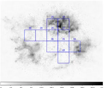
0 10 40 91 162 254 366 498 651 824 10 36 35 34 30 29 43 28 27 20 19
Fig. 9: Counts image of the Fe-K red-shifted component over-laid with the extraction regions used for the44Ti NuSTAR study of Grefenstette et al. (2017). The regions 19 and 20 which dom-inate our image in terms of flux have respective velocities mov-ing away from the observer of 2300 ± 1400 and 3200 ± 500 km sec−1.
determined in Table 2 contradict this hypothesis, as the blue-shifted clumps seem to move faster.
4.4. Comparison with44Ti
44Ti is a product of Si burning and is thought to be synthesized in close proximity with iron. The 44Ti spatial distribution has been studied via its radioactive decay with the NuSTAR tele-scope and revealed that most of the material is red-shifted and does not seem to follow the Fe-K X-ray emission (Grefenstette et al. 2014, 2017). In our study, we have found that 70% of the Fe-K X-ray emission (see Table 1) is red-shifted and that the mean direction of the Fe-K red-shifted emission shown in Fig. 6 is compatible with that of the44Ti as determined in Fig. 13 of Grefenstette et al. (2017). Yet, we can see the mean44Ti direc-tion is not perfectly aligned with the mean red-shifted Fe-K di-rection. This may be caused by the fact that the Fe-K emission is tracing only the reverse shock-heated material and may not reflect the true distribution of Fe, whereas44Ti emission is from radioactive decay and thus reflects the true distribution of Ti.
In Fig. 9, we overlay the ten regions where Grefenstette et al. (2017) detected44Ti with our red-shifted component image. The regions 19 and 20 (which dominate our Fe-K red-shifted compo-nent image) have respective44Ti velocities of 2300 ± 1400 and 3200 ± 500 km s−1, values that are compatible with our mea-sured value of ∼2800 km s−1shown in Table 2.
Concerning our Fe-K blue-shifted component map, its X-ray emission is fainter and located mostly in the South-East of the source (see Fig 3). This South-East X-ray emission is spatially coincident with region 46 in the Fig. 2 NuSTAR map of Grefen-stette et al. (2017), not plotted in our Fig 9 as the44Ti emission was found to be below the detection threshold.
Note that blue-shifted 44Ti emission is harder to detect for NuSTARthan a red-shifted one as it is intrinsically fainter. In addition, any blue-shifted emission of the 78.32 keV 44Ti line places it outside the NuSTAR bandpass, precluding detection of one of the two radioactive decay lines in this case.
5. Conclusions
By using a new methodology and applying it to Cas A Chandra X-ray data, we were able to revisit the mapping of the heavy elements and separate them into a red- and a blue-shifted parts, allowing us to investigate the three-dimensional morphology of the SNR. These new maps and the associated spectra could then be used to quantify the asymmetries of each component, their mean direction and their velocity. The main findings of the paper are summarized below :
– Morphological Asymmetries : An extensive study of the asymmetries shows the distribution of heavier elements is generally more elliptical and mirror asymmetric in Cas A, which is consistent with simulation predictions. For the ele-ments we were able to separate into a red- and a blue-shifted parts (Si, S, Ar, Ca, Fe), it appears that the red-shifted ejecta is less asymmetric than the blue-shifted one. The red-shifted ejecta can then be described as a broad, relatively symmetric plume, while the blue-shifted ejecta can be seen as concen-trated into dense knots. Most of the emission from each el-ement is red-shifted, implying there was more mass ejected away from the observer which agrees with past studies. – Three-dimensional Distribution : The mean directions
of the red- and blue- shifted parts of each element are clearly not diametrically opposed, disfavouring the idea of a jet/counter-jet explosion mechanism. The angles between the red- and blue-shifted parts become wider with increasing element mass, indicating that elements formed closer to the core and proto-NS experience stronger asymmetric forces. – NS Velocity : The NS is moving directly opposite to the
di-rection of the red-shifted ejecta which forms the bulk of the ejecta emission, supporting the idea of a ’Gravitational Tug-boat Mechanism’ of generating NS kicks. However, we find the blue-shifted clumps to be faster than the red-shifted ones, which is not fully consistent with the gravitational tug-boat mechanism.
– Comparison with44Ti : Our finding that the bulk of ejecta is red-shifted and moving NW is consistent with the44Ti dis-tribution from NuSTAR observations. Its direction is similar to that of the red-shifted Fe-K emission, but a slight di ffer-ence could be explained by the fact that the Fe-K only traces the reverse shock-heated ejecta and not the full distribution of the Fe ejecta.
The component separation method presented here enabled a three-dimensional view of the Cas A ejecta despite the low en-ergy resolution of the Chandra CCDs. In the future, X-ray mi-crocalorimeters will enable kinematic measurements of X-ray emitting ejecta in many more SNRs. In its short operations, the Hitomimission demonstrated these powerful capabilities. In par-ticular, in a brief 3.7-ks observation, it revealed that the SNR N132D had highly redshifted Fe emission with a velocity of ∼800 km s−1 without any blueshifted component, suggesting the Fe-rich ejecta was ejected asymmetrically (Hitomi Collab-oration et al. 2018). The upcoming replacement X-ray Imaging and Spectroscopy Mission XRISM will offer 5–7 eV energy res-olution with 3000 pixels over a 30 field of view (Tashiro et al. 2018). In the longer term, Athena and Lynx will combine this su-perb spectral resolution with high angular resolution, fostering a detailed, three-dimensional view of SNRs that will revolution-ize our understanding of explosions (Lopez et al. 2019; Williams et al. 2019). While the new instruments will provide a giant leap forward in terms of data quality, development of new analysis methods are needed in order to maximise the scientific return of next generation telescopes.
Acknowledgements. This research made use of Astropy,2 a community-developed core Python package for Astronomy (Astropy Collaboration et al. 2013; Price-Whelan et al. 2018) and of gammapy,3a community-developed core
Python package for TeV gamma-ray astronomy (Deil et al. 2017; Nigro et al. 2019). We also acknowledge the use of Numpy (Oliphant 2006) and Matplotlib (Hunter 2007).
References
Astropy Collaboration, Robitaille, T. P., Tollerud, E. J., et al. 2013, A&A, 558, A33
Bobin, J., Rapin, J., Larue, A., & Starck, J.-L. 2015, IEEE Transactions on Signal Processing, 63, 1199
Bruenn, S. W., Lentz, E. J., Hix, W. R., et al. 2016, ApJ, 818, 123 Buote, D. A. & Tsai, J. C. 1995, ApJ, 452, 522
Deil, C., Zanin, R., Lefaucheur, J., et al. 2017, in International Cosmic Ray Con-ference, Vol. 301, 35th International Cosmic Ray Conference (ICRC2017), 766
DeLaney, T., Rudnick, L., Stage, M. D., et al. 2010, ApJ, 725, 2038 Efron, B. 1979, Volume 7, Number 1, 1-26
Ferrand, G., Warren, D. C., Ono, M., et al. 2019, The Astrophysical Journal, 877, 136
Fesen, R. A. 2001, ApJS, 133, 161
Fesen, R. A., Hammell, M. C., Morse, J., et al. 2006, The Astrophysical Journal, 645, 283
Fesen, R. A., Morse, J. A., Chevalier, R. A., et al. 2001, AJ, 122, 2644 Foster, A. R., Ji, L., Smith, R. K., & Brickhouse, N. S. 2012, ApJ, 756, 128 Gessner, A. & Janka, H.-T. 2018, The Astrophysical Journal, 865, 61 Grefenstette, B. W., Fryer, C. L., Harrison, F. A., et al. 2017, ApJ, 834, 19 Grefenstette, B. W., Harrison, F. A., Boggs, S. E., et al. 2014, Nature, 506, 339 Hines, D. C., Rieke, G. H., Gordon, K. D., et al. 2004, ApJS, 154, 290 Hitomi Collaboration, Aharonian, F., Akamatsu, H., et al. 2018, PASJ, 70, 16 Holland-Ashford, T., Lopez, L. A., & Auchettl, K. 2020, ApJ, 889, 144 Hunter, J. D. 2007, Computing in Science & Engineering, 9, 90 Hwang, U. & Laming, J. M. 2012, ApJ, 746, 130
Hwang, U., Laming, J. M., Badenes, C., et al. 2004, ApJ, 615, L117 Janka, H.-T. 2017, ApJ, 837, 84
Janka, H.-T., Melson, T., & Summa, A. 2016, Annual Review of Nuclear and Particle Science, 66, 341
Jerkstrand, A., Wongwathanarat, A., Janka, H. T., et al. 2020, arXiv e-prints, arXiv:2003.05156
Lopez, L., Williams, B. J., Safi-Harb, S., et al. 2019, BAAS, 51, 454 Lopez, L. A., Ramirez-Ruiz, E., Badenes, C., et al. 2009, ApJ, 706, L106 Lopez, L. A., Ramirez-Ruiz, E., Huppenkothen, D., Badenes, C., & Pooley, D. A.
2011, ApJ, 732, 114
Lopez, L. A., Ramirez-Ruiz, E., Pooley, D. A., & Jeltema, T. E. 2009, The As-trophysical Journal, 691, 875
Müller, B. 2016, Publications of the Astronomical Society of Australia, 33, e048 Müller, B., Tauris, T. M., Heger, A., et al. 2019, Monthly Notices of the Royal
Astronomical Society, 484, 3307–3324
Nigro, C., Deil, C., Zanin, R., et al. 2019, A&A, 625, A10
Oliphant, T. E. 2006, A guide to NumPy, Vol. 1 (Trelgol Publishing USA) Orlando, S., Miceli, M., Pumo, M. L., & Bocchino, F. 2016, ApJ, 822, 22 Patnaude, D. J. & Fesen, R. A. 2014, The Astrophysical Journal, 789, 138 Picquenot, A., Acero, F., Bobin, J., et al. 2019, A&A, 627, A139
Price-Whelan, A. M., Sip˝ocz, B. M., Günther, H. M., et al. 2018, AJ, 156, 123 Schure, K. M., Vink, J., García-Segura, G., & Achterberg, A. 2008, ApJ, 686,
399
Summa, A., Janka, H.-T., Melson, T., & Marek, A. 2018, ApJ, 852, 28 Tashiro, M., Maejima, H., Toda, K., et al. 2018, in Society of Photo-Optical
In-strumentation Engineers (SPIE) Conference Series, Vol. 10699, Space Tele-scopes and Instrumentation 2018: Ultraviolet to Gamma Ray, 1069922 Thorstensen, J. R., Fesen, R. A., & van den Bergh, S. 2001, AJ, 122, 297 Williams, B., Auchettl, K., Badenes, C., et al. 2019, BAAS, 51, 263
Willingale, R., Bleeker, J. A. M., van der Heyden, K. J., Kaastra, J. S., & Vink, J. 2002a, A&A, 381, 1039
Willingale, R., Bleeker, J. A. M., van der Heyden, K. J., Kaastra, J. S., & Vink, J. 2002b, A&A, 381, 1039
Wongwathanarat, A., Janka, H.-T., & Müller, E. 2013, A&A, 552, A126 Wongwathanarat, A., Janka, H.-T., Müller, E., Pllumbi, E., & Wanajo, S. 2017,
ApJ, 842, 13
2 http://www.astropy.org
Appendix A: Ionization impact on line centroid
At the spectral resolution of CCD type instruments, most emis-sion lines are not resolved and the observed emisemis-sion is a blurred complex of lines. The centroid energy of emission lines can shift either via Doppler effect or when the ionization timescale in-creases and the ions distribution in a given line complex evolves. In Fig. A.1 we compare the spectral model pshock at different ionization timescales with the spectra that we labeled red- and blue-shifted in Fig. 3. The temperature of the model was fixed to 1.5 keV based on the temperature histogram of Fig. 2 of Hwang & Laming (2012). The effective area and redistribution matrix from observation ObsID : 4634 were used. We can see that as the ionization time scale τ increases the line centroid, which is a blend of multiple lines, shifts to higher energies. This is most vis-ible in the Fe-K region where a large number of lines exists. We note that the spectral component that we labeled as blue-shifted is well beyond any ionization state shown here and reinforces the idea that this component is dominated by velocity effect. The situation is less clear for the red-shifted component where the shift in energy is not as strong. We also do not precisely know which reference line it can be compared to. It is interesting to note that for the purpose of measuring a velocity effect while minimizing the confusion with ionization effects, the Ar and Ca lines provide the best probe. Indeed for τ > 1011cm−3s, the cen-troid of the main Ar and Ca lines shows no evolution given the CCD energy resolution. The Fe K centroid strongly varies with τ and the choice of a reference ionization state and reference en-ergy limits the reliability of this line for velocity measurements in non-equilibrium ionization plasma.
Appendix B: Retrieving error bars for a non-linear estimator applied on a Poissonian data set
Appendix B.1: Introduction
The BSS method we used in this paper, the pGMCA, is one of the numerous advanced data analysis methods that have recently been introduced for a use in astrophysics, among which we can also find other BSS methods, classification, PSF deconvolution, denoising or dimensionality reduction.
We can formalize the application of these data analysis meth-ods by writingΘ = A(X) , where X is the original data, A is the non-linear analysis operator used to process the signal and Θ is the estimator for which we want to find errors (in this paper for example, X is the original X-ray data from Cas A, A is the pGMCA algorithm and Θ represents the retrieved spectra and images). Most of these methods being non-linear, there is no easy way to retrieve error bars or a confidence interval associated with the estimatorΘ. Estimating errors accurately in a non-linear problem is still an open question that goes far beyond the scope of astrophysical applications, as there is no general method to get error bars from a non-linear data-driven method such as the pGMCA. This is a hot topic whose study would be essential for an appropriate use of complex data analysis methods in retriev-ing physical parameters, and for allowretriev-ing the user to estimate the accuracy of the results.
Appendix B.2: Existing methods to retrieve error bars on Poissonian data sets
Our aim, when searching for error bars associated to a certain estimatorΘ on an analyzed data set, is to obtain the variance of Θ = A(X) , where the original data X is composed of N elements.
Fig. A.1: Comparison of our red/blue spectra (dotted curves) pre-sented in Fig. 3 versus pshock Xspec models with different ion-ization timescales for kT=1.5 keV.
When working on a simulation, an obvious way to proceed in or-der to estimate the variance ofΘ is to apply the considered data analysis method A on a certain number of Monte-Carlo (MC) realizations Xi and look at the standard deviation of the results
Original data First bootstrap resampling
Second bootstrap resampling
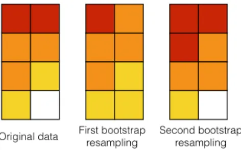
Fig. B.1: An example of bootstrap resampling. Each square rep-resents a different event, each color a different value. N events are taken randomly with replacement from the original data to create each of the two bootstrap resamplings.
Θi = A(Xi). The variance of theΘiprovides a good estimation of the errors. Yet, this cannot be done with real data, as only one observation is available : the observed one. Thus, a resampling method such as the jackknife, the bootstrap (see Efron 1979) or its derivatives, able to simulate several realizations out of a single one, is necessary. Ideally, the aim is to obtain through this resampling method a number of ”fake” MC realizations centered on the original data : new data sets variating spatially and repro-ducing the spread of MC drawings with a mean equal or close to the mean of the original data.
The mechanisms at stake in jacknife or bootstrap resam-plings are similar. Jacknife and bootstrap resampling methods produce n resampled sets ˜Xiby rearranging the elements of X, and allow us to consider the variance ofΘi= A( ˜Xi) for i in ~1, n as an approximation for the variance ofΘ. As jacknife and boot-strap methods are close to each other, and the bootboot-strap and some of its derivatives are more adapted to handle correlated data sets, we will in this Appendix focus on a particular method, repre-sentative of other resampling methods and theoretically suited for astrophysical applications : the block bootstrap, which is a simple bootstrap applied on randomly formed groups of events rather than on the individual events.
In the case of a Poisson process, the discrete nature of the elements composing the data set can easily be resampled with a block bootstrap method. The N discrete elements composing a Poissonian data set X will be called "events". In X-rays for exam-ple, the events are the photons detected by the spectro-imaging instrument. The bootstrap consists in a random sampling with replacement from the current set events X. The resampling ob-tained through bootstrapping is a set ˜Xbootof N events taken ran-domly with replacement amid the initial ones (see Fig. B.1). This method can be repeated in order to simulate as many realiza-tions ˜Xibootas needed to estimate standard errors or confidence intervals. In order to save calculation time, we can choose to re-sample blocks of data of a fixed size instead of single events : this method is named block bootstrap. The block bootstrap is also supposed to conserve correlations more accurately, making it more appropriate for a use on astrophysical signals. The data can be of any dimension but for clarity, we will only show in this Appendix bi-dimensional data sets, i.e. images.
Appendix B.3: Biases in classical bootstrap applied on Poissonian data sets
The properties of the data resampled strongly depends on the na-ture of the original data. Biases may appear in the resampled data sets, proving a block bootstrap can fail to reproduce consistent
data that could be successfully used to evaluate the accuracy of certain estimators.
In particular, Poissonian data sets, including our X-rays data of Cas A, are not consistently resampled by current resampling methods such as the block bootstrap. A Poissonian data set X can be defined as a Poisson realization of an underlying theoretical model X∗, which can be written :
X= P(X∗)
where P(.) is an operator giving as an output a Poisson realiza-tion of a set.
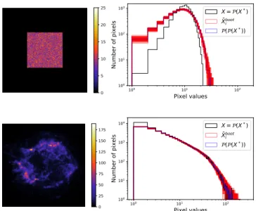
A look on the histogram of a data set resampled from a Pois-sonian signal shows the block bootstrap fails to reproduce ac-curately the characteristics of the original data. Fig. B.2, top, compares the histogram of the real data X, a simple image of a square with Poisson noise, with the histograms of the resampled data sets ˜Xboot
i , and highlights the fact that the latter are more similar to the histogram of a Poisson realization of the origi-nal data P(X) = P(P(X∗)) than to the actual histogram of the original data X = P(X∗), where X∗is the underlying model of a square before adding Poisson noise. This is consistent with the fact that the block bootstrap is a random sampling with re-placement, which introduces uncertainties of the same nature as a Poisson drawing.
Fig. B.2, bottom, shows the comparison between the his-togram of the toy model Cas A image and the hishis-tograms of the data sets resampled with a block bootstrap. We can see the re-sampling is, in this case too, adding Poissonian noise and gives histograms resembling P(P(X∗)) rather than P(X∗). The same goes with our real data cube of Cas A : Fig. B.3 shows an obvi-ous instance of this bias being transferred to the results of the pGMCA, thus proving the block bootstrap cannot be used as such to retrieve error bars for this algorithm.
Appendix B.4: A new constrained bootstrap method
Bootstrap resamplings consisting in random drawings with re-placement, it is natural that they fail to reproduce some charac-teristics of the data, among which the histogram that gets closer to the histogram of a Poisson realization of the original data than to the histogram of the actual data. The block bootstrap method is therefore unable to simulate a MC centered on the original data : the alteration of the histogram strongly impacts the nature of the data, hence the differences in the morphologies observed by looking at the wavelet coefficients. It is then necessary to find a new method in which we could force the histogram of the re-sampled data sets to be similar to that of the original data.
A natural way to do so would be to impose the histogram we want the resampled data to have before actually resampling the data. To allow this constraint to be made on the pixel distribu-tion, we can no longer consider our events to be the individual elements of X or a block assembling a random sample of them. We should directly work on the pixels and their values, the pix-els here being the basic bricks constituting our data. Just as the block bootstrap, our new method can work with data of any di-mension. In the case of images, the "basic bricks" correspond to actual pixels values. In the case of X-rays data cubes, they are tiny cubes of the size of a pixel along the spatial dimensions, and the size of an energy bin along the spectral dimension. The same goes for any dimension of our original data. The method can also be adapted for uni-dimensional data sets. The key of our new method is then to work on the histogram of the data presenting the pixels’ values rather than on the data itself, event by event.
0 5 10 15 20 25 100 101 102 Pixel values 100 101 102 103 Number of pixels X = (X*) Xbooti ( (X*)) 0 25 50 75 100 125 150 175 100 101 102 Pixel values 100 101 102 103 104 Number of pixels X = (X*) Xbooti ( (X*))
Fig. B.2: Data sets and their associated histogram in two cases : on top, the very simple case of a Poisson realization of the image of a square with uniform value 10 ; on the bottom, a toy model Cas A image obtained by taking a Poisson realization of a high-statistics denoised image of Cas A (hereafter called toy model). On the right, the black histogram correspond to the original data X = P(X∗). The red histograms are those of the data sets ˜Xboot
i obtained through resampling of the original data and the blue ones are the histograms of a Poisson realization of the original data P(X) = P(P(X∗)). It appears that the resampled data sets have histograms highly similar to that of the original data with additional Poisson noise.
5.50 5.75 6.00 6.25 6.50 6.75 7.00 7.25 7.50
E (keV)
2000 4000 6000 8000 10000 12000 14000 16000 18000Total counts
Real data
Resampled data
Fig. B.3: Spectrum of the synchrotron component retrieved by pGMCA on the 5.5-7.5 keV energy band on real data and on a set of 30 block bootstrap resamples. There is an obvious bias in the results, the resampled data spectra being consistently under-estimated.
We can either change the value of a pixel or exchange the value of a pixel for that of another one. The first operation si-multaneously adds and subtracts 1 in the corresponding columns of the global histogram while the second operation does not pro-duce any change in it. A good mixture of these two operations would then allow us to obtain the histogram we want to impose in our resampled data sets, and following a Poisson probability
Step 1 :
Step 2 :
Original image
Defining a new histogram
Imposing the new histogram on the original image
Fig. B.4: Scheme resuming the two steps of our new constrained bootstrap method. 100 101 102 103 Pixel values 101 100 101 102 103 104 105 Number of pixels Constrained bootstrap Monte-Carlo Original data 100 101 102 103 Pixel values 101 100 101 102 Standard deviation Constrained bootstrap Monte-Carlo
Fig. B.5: On the left, histogram of the original data, the resam-pled data sets and the MC realizations of the toy model Cas A image. On the right, the standard deviations of the resampled data sets and MC realizations bin by bin of the histogram on the left. We can notice the great adequation between the standard deviations of the resampled data sets and that of the MC realiza-tions.
law to select the pixels to exchange would introduce some spatial variations, in order to reproduce what a MC would do.
Our new constrained bootstrap method is thus composed of two steps, that are described below and illustrated in Fig. B.4 :
– Obtaining the probability density function of the random variable underlying the observed data histogram using the Kernel Density Estimation (KDE), and randomly generating nhistograms from this density function with a spread around the data mimicking that of a MC, with a constraint enforcing a Poissonian distribution of the total sums of pixel values of the n histograms.
– Producing resampled data sets associated with the new his-tograms by changing the values of wisely chosen pixels in the original image.
During these steps, the pixels equal to zero remain equal to zero, and the non-zero pixels keep a strictly positive value. This constraint enforces the number of non-zero pixels to be constant and avoids the creation of random emergence of non-zero pix-els in the empty area of the original data. While this is not com-pletely realistic we prefer constraining the resampled data sets in this way than getting spurious features. We could explore ways to release this constraint in the future.
Fig. B.5 highlights the similarities between the original his-togram and those obtained through MC realizations and our new constrained bootstrap resamplings, while Fig. B.6 and the spec-tra in Fig. 3 and Fig. 8 show that even after being processed by
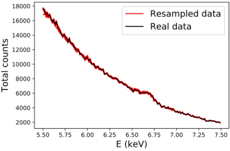
5.50 5.75 6.00 6.25 6.50 6.75 7.00 7.25 7.50
E (keV)
2000 4000 6000 8000 10000 12000 14000 16000 18000Total counts
Resampled data
Real data
Fig. B.6: Spectrum of the synchrotron component retrieved by pGMCA on the 5.5-7.5 keV energy band on real data and on a set of 100 constrained bootstrap resamples. The bias we observed in Fig. B.3 between the real Cassiopeia A data and its block boot-strap resamples has been suppressed with our new constrained bootstrap method.
the sensitive pGMCA algorithm, this resampling method shows little to no biases. Hence, our new constrained bootstrap method brings a first and successful attempt at solving the problem of biases in bootstrapping Poissonian data sets.
The comparison of our resampled data sets to a group of MC realizations of the same simulation of Cas A appears to be promising for the variance induced by our method. However, when applying a complex estimator such as the pGMCA on both the MC realizations and our resampled data sets, it appears that the variances obtained through our method fail to accurately re-produce those of the MC realizations. For that reason, the error bars retrieved by our constrained bootstrap method do not have a physical signification. Nevertheless, they constitute an interest-ing way to assess the robustness of our method around a certain line emission. The different resamplings explore initial condi-tions slightly different from the original data, thus evaluating the dependence of our results on the initial conditions. Fig. 3 and Fig. 8 indeed show that for some line emissions, the dispersion between the results on different resampled data sets is far greater than for others.
This new constrained bootstrap method is a first and promis-ing attempt at retrievpromis-ing error bars for non-linear estimators on Poissonian data sets, a problem that is often not trivial. In non-linear processes, errors frequently cannot be propagated cor-rectly, so the calculation of sensitive parameters and the estima-tion of errors after an extensive use of an advanced data analysis could benefit from this method. We will work in the future on a way to constraint the variance of the results to be more closely related to that of a set of MC realizations in order to ensure the physical signification of the obtained error bars.