Root systems, spectral curves, and analysis of a Chern-Simons matrix model for Seifert fibered spaces

HAL Id: cea-01278006

https://hal-cea.archives-ouvertes.fr/cea-01278006

Preprint submitted on 23 Feb 2016

HAL is a multi-disciplinary open access

archive for the deposit and dissemination of

sci-entific research documents, whether they are

pub-lished or not. The documents may come from

teaching and research institutions in France or

abroad, or from public or private research centers.

L’archive ouverte pluridisciplinaire HAL, est

destinée au dépôt et à la diffusion de documents

scientifiques de niveau recherche, publiés ou non,

émanant des établissements d’enseignement et de

recherche français ou étrangers, des laboratoires

publics ou privés.

Root systems, spectral curves, and analysis of a

Chern-Simons matrix model for Seifert fibered spaces

Gaëtan Borot, Bertrand Eynard, Alexander Weiße

To cite this version:

Gaëtan Borot, Bertrand Eynard, Alexander Weiße. Root systems, spectral curves, and analysis of a

Chern-Simons matrix model for Seifert fibered spaces. 2016. �cea-01278006�

IPhT T14/100 CRM-3339

Root systems, spectral curves, and analysis of a Chern-Simons

matrix model for Seifert fibered spaces

Ga¨etan Borot123_{, Bertrand Eynard}45

with a section by Alexander Weisse3

Abstract

We study a class of scalar, linear, non-local Riemann-Hilbert problems (RHP) involving finite sub-groups of PSL2pCq. We associate to such problems a (maybe infinite) root system and describe the

relevance of the orbits of the Weyl group in the construction of its solutions. As an application, we study in detail the large N expansion of SUpN q and SOpN q{Spp2N q Chern-Simons partition function ZNpM q of 3-manifolds M that are either rational homology spheres or more generally Seifert fibered

spaces. It has a matrix model-like representation, whose spectral curve can be characterized in terms of a RHP as above. When π1pM q is finite (i.e. for manifolds M that are quotients of S3 by a finite

isometry group of type ADE), the Weyl group associated to the RHP is finite and the spectral curve is algebraic and can be in principle computed. We then show that the large N expansion of ZNpM q

is computed by the topological recursion. This has consequences for the analyticity properties of SU{SO{Sp perturbative invariants of knots along fibers in M .

Contents

1 Introduction 1

2 The matrix model 5

3 Algebraic theory of sheet transitions 9

4 Seifert fibered spaces and Chern-Simons theory 17

5 Spectral curve and 2-point function : inhomogeneous part 26

6 Spectral curve and 2-point function: case study 29

7 Topological recursion 57

8 Generalization to SO and Sp Chern-Simons 62

1_{Section de Math´ematiques, Universit´e de Gen`eve, 2-4 rue du Li`evre 1206 Gen`eve, Switzerland.} 2_{MIT, Maths Department, Massachusetts Avenue 77, Cambridge 02139, USA}

3_{Max Planck Institut f¨ur Mathematik, Vivatsgasse 7, 53111 Bonn, Germany.}

4_{Institut de Physique Th´eorique, CEA Saclay, Orme des Merisiers, 91191 Gif-sur-Yvette, France.} 5_{Centre de Recherches Math´ematiques, 2920, Chemin de la Tour, Montr´eal, QC, Canada.}

9 Numerical estimates of equilibrium distributions 71

A Proofs of Section 2 82

B Finite subgroups of PSL2pCq 85

C Case p2, 3, 3q: matrices of singularities 85

D p2, 3, 4q case: polynomial equations 86

E p2, 3, 5q case: additional formulas 88

*

Acknowledgements

G.B. thanks Andrea Brini, R´eda Chhaibi, Thomas Haettel, Neil Hoffman, Thang Lˆe, Alexei Oblomkov, George Thompson, and especially Albrecht Klemm, Stavros Garoufalidis and Marcos Mari˜no for com-ments and fruitful discussions, as well as the organizers of the Quantum Topology and Hyperbolic Ge-ometry conference in Nha Trang (May 2013), where a preliminary version of this work was presented. Marcos Mari˜no and Alba Grassi collaborated in an earlier phase to the Section 8 concerning Kauffman invariants. This work benefited from the support of Fonds Europ´een S16905 (UE7–CONFRA), the Swiss NSF, the Max-Planck-Gesellschaft, and the Simons foundation.

B.E. thanks T. Kimura, the CRM Montr´eal, the FQRNT grant from the Qu´ebec government, P. Su lkowski and the ERC starting grant Fields-Knots, S. Smirnov and the University of Geneva. AMS Classification: 14Hxx, 45Exx, 51Pxx, 57M27, 60B20, 81T45.

1

Introduction

Unless mentioned otherwise, the orbit space of Seifert fibered spaces in this article is assumed to be a sphere.

1.1

Scope

g_{denotes a semi-simple Lie algebra, and h its Cartan subalgebra, identified with R}N_{. We shall study}

the probability measure over t “ pt1, . . . , tNq P h:

dµptq “ 1 Zg_{pM q} « ź αą0 sinh2´r` α¨ t 2 ˘ r ź m“1 sinh` α¨ t 2am ˘ ff _N ź j“1 e´N V ptjq_dt j, V ptq “ t2 2u. (1.1) where the product ranges over positive roots of g, u is a positive parameter, and the partition function ZgpM q is such that´_hdµptq “ 1. We are interested in the AN, BN, CN, DN series of Lie algebras, in

the regime where the rank N goes to 8.

The model (1.1) arises in Chern-Simons theory with gauge group exppgq on a simple class of 3-manifolds M called Seifert fibered spaces [38_{]: roughly speaking, these are S}1-fibrations over a surface

orbifold, here assumed to be topologically a sphere. (1.1) captures the contribution of the trivial flat connection in perturbative Chern-Simons theory, or equivalent, the evaluation of the LMO invariants of M in the weight system defined by g [37,1, 2, 2, 3]. Moreover, the correlation functions in (1.1)

compute the colored HOMFLY (in any representation of fixed size) of the knots going along the fibers of M , see § 4.4. The regime N Ñ 8 has aroused interest since it allows a rigorous definition of perturbative invariants ensuing from Z_NgpM q and the colored HOMFLY of links in M , which should be related via geometric transitions to topological strings invariants in T˚_{M according to the physics}

literature [47], see §1.4.

General arguments [14] show that the large N asymptotic expansion of models of the type (1.1) – once it is proven to exist using the tools of [15] – can be computed by the topological recursion of [22]. It then remains to compute the initial data pω0,1, ω0,2q of the recursion : ω0,1 is related to the

equilibrium measure of (2.1), also called spectral curve, and ω0,2 is related to the large N limit of the

2-point correlation function. Both are characterized by a saddle point equation which takes the form of a linear but non-local Riemann-Hilbert problem (RHP) on a cut locus to determine. Addressing its solution is an important part of our present work. We shall devise in Section 3 a general method to construct the solution of a large class of RHP where the jumps are obtained by action of a finite subgroup of M¨obius transformations. We actually build the – maybe infinite – monodromy group of the solution, and relate it to the Weyl group of a root system. The solution can be studied in more details by algebro-geometric means when this Weyl group is finite. This construction applies to the computation of pω0,1, ω0,2q relevant for (2.1), but has also its own interest and can be used as a tool

in other problems.

Our work has two noteworthy consequences for knot theory.

Firstly, we obtain analyticity results on perturbative invariants of knots in manifolds different from the 3-sphere. The colored HOMFLY of links in S3 are polynomials (after a suitable normalization)

in q and qN. This is clear from skein theory, and can also be explained from quantum field theory perspective [48_{]. This implies that the coefficients in the ~ Ñ 0 expansion while keeping q}N

“ eu0

fixed, produce polynomials in eu0_{. These properties are not expected to be true for invariants of}

links in other 3-manifolds. We show how to compute invariants of fiber knots in Seifert fibered spaces. Remarkably, the position of the singularities in the u “ N ~-complex plane only depend on the ambient 3-manifold. They occur at the singularities of the family of spectral curves (parametrized by u) associated to (1.1). We conjecture more generally that for any link in a rational homology sphere M , the singularities of the perturbative invariants only depend on the ambient manifold M . More precise statements of the conjecture described in §4.2.2.

Secondly, we find that the spectral curves and the perturbative invariants for the colored Kauffman perturbative invariants (associated to the BN, CN, DN Lie algebra) are closely related to the more

conventional SUpN q invariants (AN ´1series), and we show they can all be computed by the topological

recursion. The only difference is that the topological grading is not respected for the BCD cases. We think this has an interest, since very few was known so far on perturbative Kauffman invariants.

1.2

Outline and main results: matrix model

We establish in Section 2 the large N Ñ 8 behavior and asymptotic expansion of the partition function and moments of (1.1) for g “ AN “ supN ` 1q (Section 2). Some of the technical proofs

are postponed to AppendixA. Section3 is independent of the main body of the text: we introduce in (3.1) a class of linear non-local RHP, to which we associate a (maybe infinite) root system. Many information on the solution – and sometimes its full and explicit form – can be extracted from the analysis of this root system.

important geometric invariant of Seifert spaces is the orbifold Euler characteristic of their orbit space, here always assumed to be topologically a sphere :

χ “ 2 ´ r ` r ÿ m“1 1 am (1.2) where a1, . . . , am are integers prescribing the orders of extraordinary fibers. We also introduce:

a “ lcmpa1, . . . , amq (1.3)

Section5-7are devoted to the AN Chern-Simons matrix model for Seifert fibered spaces, and their

extension to the Sp or SO Lie algebra is the matter of Section 8. Chern-Simons theory around the trivial flat connection depends on the single parameter:

u “ N ~{σ (1.4)

where σ P Q is another geometric parameter of the Seifert spaces. u0 “ N ~ is sometimes called the

string coupling constant. In Section 5, we apply the techniques of Section3 to the construction of the spectral curves for Seifert spaces. We find in Theorem6.1_{that the finite quotients M “ Z}pzS3{H

corresponding to χ ą 0 can be described in terms of an algebraic spectral curve S ãÑ Cˆ

ˆ Cˆ, whereas the spectral curve – if it exists – is never algebraic when χ ă 0. We will not insist on the cases χ “ 0, which are resonant.

Proposition 1.1 The Chern-Simons matrix model for Seifert fibered spaces with χ ą 0 admits a spectral curve S of the form P px, yq “ 0 for a u-dependent polynomial P whose Newton polygon is known. The coefficients on the boundary of the Newton polygon are known monomials in e´χu{2a_.

Besides, the spectral curve comes with the action of a finite Weyl group on the sheets of x : S Ñ pC, as tabulated below.

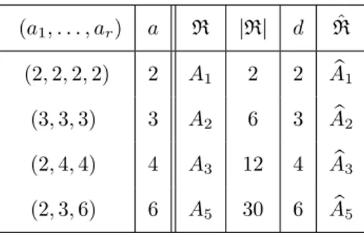
Geometry pa1, . . . , arq degxP degyP genus Weyl group

Lpa1, a2q pa1, a2q a1a2 a1` a2 pa1´ 1qpa2´ 1q Aa1`a2´1 S3{Dp`2 pp oddq p2, 2, pq 4p 2pp ` 1q 2p ` 1 Dp`1 S3{Dp`2 pp evenq p2, 2, pq 2p p ` 1 0 Ap S3{E6 p2, 3, 3q 8 8 5 D4 S3{E7 p2, 3, 4q 36 27 46 E6 S3{E8 p2, 3, 5q 540 240 1471 E8

This table assumes gcdpa1, a2q “ 1 for the lens spaces.

We were able in Section6:

‚ to determine completely the curves in the cases S3{Dp`2– corresponding to p2, 2, p ´ 2q, in §6.2

and6.3.

‚ to determine the curves in the cases S3{E6(resp. S3{E7) up to 2 (resp. 4) parameters fixed by

complicated algebraic constraints.

Our spectral curve computations are supported by Monte-Carlo simulations of Alexander Weisse presented in Section 9. Bases on numerics, we also give conjectures about the spectral curve in the cases χ ă 0 (Conjecture2.5).

Although the genus of the spectral curve can be quite large, it does not prevent them to cover in a simple way curves of a lower genus. The completely solved cases mentioned above and our computations leads us to:

Conjecture 1.2 Assume χ ą 0. In the spectral curves describing the contribution of the trivial flat connection to the Chern-Simons partition function, if one eliminates x from the equations X “ xa _and

P px, yq “ 0, we obtain an equation RpX, yq “ 0 describing a (in general : singular and with several components) curve of genus 0.

This is true for the S3{Dp cases. Some formulas and definitions met during those computations are

collected in AppendicesE-C.

1.3

Outline and main results: knot theory

In Section 7, we explain a practical consequence for knot theory: we can provide some informations on the analyticity properties of the coefficients (seen as functions of eu_{) of the large N expansion of}

the colored HOMFLY polynomials of fiber knots in M , and of the Chern-Simons free energy. So far, they were only known to be analytic in a vicinity of u “ 0 [26]. We prove in Section7:

Proposition 1.3 The perturbative colored HOMFLY invariants of fiber knots in a Seifert fibered space with geometry S3{Dp`2for p even, defined initially as elements of Qrr~ssrru0ss, are actually the u0Ñ 0

Taylor expansion of an element Qrr~sspκ2qraβpκqs, where: 2κ1`1{p 1 ` κ2 “ e ´u0{p4σp2q_{, βpκq “} pκ 2 ` 1qppp ` 1q ´ pp ´ 1qκ2q κ2 (1.5)

u0 ą 0 corresponds to κpu0q Ps0, 1r, and σ P Q introduced in (4.3) is a geometric parameter of the

Seifert spaces. The singularities in the κ-complex plane occur when κ4P t1, pκ˚q4u where:

κ˚

“c p ` 1

p ´ 1 (1.6)

A result similar to Proposition 1.3, with u replaced by 2u, can be deduced from Section 7-8 for the perturbative colored Kauffman invariant of fiber knots in S3{Dp`2 with p even.

The situation is different from links in lens spaces, where the perturbative invariants are polyno-mials in eu [17], and thus had no singularities in the u-complex plane. Our work suggests the general conjectures:

Conjecture 1.4 If M is a Seifert fibered space, the Fpgq _{and the perturbative invariants of any link}

in M exist as a function of u0ą 0, and are real-analytic on the positive real line.

Conjecture 1.5 Moreover, if χ ą 0, there exists a finite degree extension L of Qpe´χu0{2σ_{q depending}

only on the ambient manifold and the series X P tA, BCDu of Lie algebra, such that, at least for fiber knots, the perturbative invariants colored in any representation are the Laurent expansion at u0Ñ 0

of elements of L.

From this perspective, for the Seifert space M “ S3{Dp with p even, one may ask for the geometric

interpretation of the function κpu0q in (1.5), and of the location of the dominant singularity u˚0 “

u0pκ˚q determined by (1.6).

1.4

Motivation from topological strings

The present work generalizes the analysis of the model r “ 2 [29, 17] relevant to study lens spaces, and the invariant of fiber knots in lens spaces are equal to invariants of torus knots in S3.

geometric transitions, this can sometimes be related to closed topological strings on another target space XM. This program has been completed for M “ S3 [28] and the lens spaces Zp2zS3{Zp1 [29,17]

and XM is obtained by fractional framing transformations from the resolved conifold in both cases.

So far, it has remained elusive for general Seifert fibered spaces. Since we establish the existence of an algebraic spectral curve for all Seifert spaces with χ ě 0, this gives hope for the construction of their mirror geometries XM. This direction, and the connection with 5d gauge theories and quantum

spectral curves, is under investigation [12].

A natural strategy to establish a duality to a closed string geometry would then be to prove that Gromov-Witten invariants of XM are also computed by the topological recursion, with same curve S.

So far, the topological recursion is indeed known to compute Gromov-Witten invariants when X is a toric 3-fold Calabi-Yau [16,23], but this might be generalized in the future to a more general class of manifolds.

2

The matrix model

2.1

Equilibrium measures

We study the statistical mechanics of N particles, of position t1, . . . , tn P RN, with joint probability

distribution: dµptq “ 1 ZN ” ź 1ďiăjďN sinh2´r` ti´ tj 2 ˘ r ź m“1 sinh` ti´ tj 2am ˘ı N ź j“1 e´N V ptjq_dt j, V ptq “ t2 2u. (2.1) At this stage, a1, . . . , arare arbitrary positive parameters. The dominant contribution to the partition

function when N Ñ 8 should come from configurations t maximizing the probability density. It is reasonable to think that the empirical distribution:

LN “ 1 N N ÿ i“1 δti (2.2)

of such configurations will be close to a minimizer of the energy functional: Erλs “ ´1 2 ¨ dλptqdλpt1 q ” p2 ´ rq lnˇˇsinh` t´ t 1 2 ˘ˇ ˇ` r ÿ m“1 lnˇˇsinh` t´ t 1 2am ˘ˇ ˇ ı ` ˆ dλptq V0ptq (2.3)

among probability measures λ. E0 is actually defined in R Y t`8u because of the singularity of the

logarithm. It is a lower semi-continuous functional, so has compact level sets for the weak-* topology, therefore it achieves its minimum. We call equilibrium measure and denote λeq any minimizer of E .

It must satisfy the saddle point equation: there exist a constant Cλeq _{such that}

Vλeq eff ptq :“ V ptq ´ ˆ dλeqpt1q ” p2 ´ rq lnˇˇsinh` t´ t 1 2 ˘ˇ ˇ` r ÿ m“1 lnˇˇsinh` t´ t 1 2am ˘ˇ ˇ ı ě Cλeq _(2.4)

with equality λeq-everywhere. Veffλptq is the effective potential felt by a particle at position t “ ti,

taking into account the collective effect of all other tj’s distributed according to λ. Equilibrium

measures are characterized by the property that the effective potential achieves its minimum on the locus of R where the particles accumulate. Classical techniques6 _{of potential theory [43] show that}

the random measure LN’s limit points are equilibrium measures, and that:

ZN “ exp

`

´ N2 min E ` opN2q˘ (2.5)

6_{The arguments of [43] were developed for the pairwise interaction}ś

iăjpti´ tjq2 which has a zero at coinciding points, but it is easy to generalize to any interaction which has the same singularity and is smooth elsewhere.

Some qualitative properties of the equilibrium measures can be derived from their characterization: V grows sufficiently fast at infinity to ensure that equilibrium measures have compact support ; since V and the pairwise interactions are analytic (away from the singularity at x “ y), it can be shown (see [15], generalizing [18] where ´ ln |t ´ t1_{| was considered) that equilibrium measures are supported on}

a finite number of segments, have a density which is analytic away from the edges, and is 1{2-H¨older at the edges. When the density vanishes exactly like a squareroot at the edges, it is said off-critical.

The question of uniqueness of µeq has no easy answer. But, since the functional is quadratic, if

the quadratic form over the space M0 of differences of probability measures: Qrνs “ ´ ¨ dνptqdνpt1_q”_{rp2 ´ rq ln}ˇ ˇsinh` t´ t 1 2 ˘ˇ ˇ` r ÿ m“1 lnˇˇsinh` t´ t 1 2am ˘ˇ ˇ ı (2.6)

is positive definite, then E is strictly concave and this guarantees uniqueness of its minimizer. Notice again that, a priori, Q takes values in R Y t`8u. Indeed, the singular part of Q is:

´ 2 ¨ dνptqdνpt1_{q ln |t ´ t}1_{| “} ˆ 8 0 |F rνspkq|2 k ě 0 (2.7)

and the right-hand side can be infinite if the measure ν is not regular enough. Here F rνs “´ dνpxq eikx is the Fourier transform of the finite mesure ν. As a matter of fact, it is enough to consider E and Q as functionals over measures with compact support, because V grows fast at infinity compared to the pairwise interactions.

Lemma 2.1 For any ν P M0: Qrνs “ ˆ 8 0 ” p2 ´ rqγpkq ` r ÿ m“1 γpamkq ı |F rνspkq|2dk k , γpkq “ cotanhpπkq. (2.8) Q is definite positive whenever the function p2 ´ rqγpkq `řr

m“1γpaikq is almost everywhere positive.

In particular, it must be positive at k Ñ 8, which gives the necessary condition: χ “ 2 ´ r ` r ÿ m“1 1 am ě 0 (2.9)

In the model for Seifert fibered spaces, the am are assigned integer values. We recognize in (2.9) the

orbifold Euler characteristics of the orbit space, and the list of uples leading to χ ě 0 is finite. For r “ 1 and r “ 2, Q is obviously positive definite, and for the remaining r “ 3 cases having χ ě 0, positivity can be checked by a direct computation.

Corollary 2.2 If a1, . . . , ar are integers, Q is definite positive iff 2 ´ r `

řr

m“1a´1m ě 0. In those

cases, there exists a unique equilibrium measure.

The proof of Lemma 2.1 and Corollary 2.2 are presented in Appendix A.1 and A.2. We can also establish – see AppendixA.3– some qualitative properties of equilibrium measures:

Theorem 2.3 For any a1, . . . , arą 1, and any u ą 0, any equilibrium measure ˇλeq is supported on

a single segment, and vanishes exactly as a squareroot at the edges (generic edge).

Corollary 2.4 If χ ě 0, since the equilibrium measure is unique, it must be invariant under t ÞÑ ´t. In particular, its support is a segment centered at the origin.

In Section 9, Weisse proposes a Monte-Carlo simulation to obtain the dominant configurations of probability densities like (2.1). It is observed that, for any value of am integers and u ą 0,

independently of the sign of χ, the empirical measure seem to have a unique limit point. It supports the

Conjecture 2.5 For any a1, . . . , arą 1 and u ą 0, the equilibrium measure is unique, and its density

away from the edges of the support is a real-analytic function of u ą 0.

2.2

Change of variable and saddle point equation

We introduce the exponential variables:

si“ eti{a, a “ lcmpa1, . . . , arq, ˇai“ a{ai (2.10)

The measure µ (2.1_{) on t P R}N transforms into a measure ˇ_{µ on pR}ˆ_`qN:

dˇµpsq “ _ˇ1 ZN ź 1ďiăjďN psi´ sjq2 ź 1ďi,jďN ˇ Rpsi, sjq1{2 N ź j“1 e´N ˇV psiq_ds i (2.11) where: ˇ V psq “ a 2 pln sq2 2u ` aχ 2 ln s, ˇ Rps, s1 q “ a´1 ź `“1 ps ´ ζa`s1q2´r r ź m“1 ˇ am´1 ź `m“1 ps ´ ζ`m ˇ ams 1 q, (2.12)

and ζa denotes a primitive ath-root of unity.

ˇ

λeq denote an equilibrium measure for ˇµ. It is the image via (2.10) of an equilibrium measure λeq

for µ. It is characterized by the saddle point equation: ˇ Veffpxq :“ ˇV pxq ´ ˆ dˇλeqpsq“2 ln |x ´ s| ` ln ˇRpx, sq ‰ ě C (2.13)

for some constant C, with equality on the support Γ Ď Rˆ

`of λeq. We shall rewrite the characterization

of an equilibrium measure in term of its Stieltjes transform: W pxq “ ˆ x dˇλeqpsq x ´ s “ limN Ñ8µˇ ”1 N Tr x x ´ S ı , S “ diagps1, . . . , sNq (2.14)

W is a bounded, holomorphic function on CzΓ, such that: `W px ´ i0q ´ W px ` i0q˘dx “ 2iπx dˇλeqpxq, lim

xÑ8W pxq “ 1, xÑ0limW pxq “ 0. (2.15)

The saddle point equation (2.13) implies a functional equation:

@x P ˚Γ, W px ` i0q ` W px ´ i0q ` ˛ Γ xBxln ˇRpx, sq W psqds 2iπs “ x ˇV 1 pxq (2.16) with: x ˇV1 pxq “ a 2<sub>ln x</sub> u ` aχ 2 . (2.17)

The contour of integration in (2.16) can be moved to pick up residues at rotations of x of order a:

@x P Γ, W px ` i0q ` W px ´ i0q ` p2 ´ rq a´1 ÿ `“1 W pζa`xq ` r ÿ m“1 ˇ am´1 ÿ `m“1 W pζ`m ˇ amxq “ x ˇV 1 pxq. (2.18)

Since µ is invariant under pt1, . . . , tNq Ñ p´t1, . . . , ´tNq, in the case where the equilibrium measure

is unique, it must have the same symmetry. This translates into the palindrome symmetry :

W pxq ` W p1{xq “ 1 (2.19)

When Q is definite positive and Γ is fixed, (2.18) characterizes W among the holomorphic functions in CzΓ satisfying (2.15) and whose discontinuity on Γ defines an integrable measure (see e.g. the argument of [14, Lemma 3.10]). When Q is not definite positive, we do not know how to address the question of uniqueness.

2.3

Asymptotic analysis

We rely on the results of [15] to study the asymptotic expansion when N Ñ 8 of the model (2.11). We would like to compute the partition function ˇZN and the n-point correlators:

Wnpx1, . . . , xnq “ ˇµ ”_źn i“1 Tr xi xi´ S ı conn (2.20)

where conn stands for ”connected expectation value”.

Definition 2.6 We say that ˇλeq is off-critical if its density is nowhere vanishing on its support Γ,

and it vanishes exactly like a squareroot at the edges of Γ.

Theorem 2.7 [15] Assume E is strictly concave and ˇλeqis off-critical. Then, we have an asymptotic

expansion of the form:

ˇ ZN “ N exp ´ ÿ gě0 N2g´2Fpgq¯ Wnpx1, . . . , xnq “ ÿ gě0 N2´2g´nWpgq n px1, . . . , xnq (2.21)

The coefficients of expansion are real analytic functions of u ě 0, and Wnpgqpx1, . . . , xnq are

holomor-phic functions in pCzΓqn_.

In particular, this confirms for Seifert spaces, by a different method, the analyticity of Chern-Simons free energies proved in general for rational homology spheres in [26] (see §4.2). From (2.11), we have the basic relation:

u2BuFpgq“ ˛ Γ dx x a2pln xq2 2 W pgq 1 pxq (2.22)

2.4

Two point function

Definition 2.8 We call 2-point function: W₂p0qpx1, x2q “ lim N Ñ8µˇ ” Tr x1 x1´ S Tr x2 x ´ S ı conn “ lim N Ñ8 ˜ ˇ µ”Tr x1 x1´ S Tr x2 x2´ S ı ´ ˇµ”Tr x1 x1´ S ı ˇ µ”Tr x2 x2´ S ı ¸ (2.23)

It can be obtained formally from W pxq “ W1p0qpxq by an infinitesimal variation of the potential ˇV :

W₂p0qpx1, x2q “ B Bεµˇ ˇ V_ε,x2” N ÿ i1“1 x1 x1´ si1 ıˇ ˇ ˇ ε“0 , Vˇε,x2pxq “ ˇV pxq ´ 1 N x2 x2´ x (2.24)

It also satisfies also a saddle point equation, which can be obtained by formally applying the variation of the potential to the saddle point equation (2.18) satisfied by W pxq. The result is that W₂p0qpx1, x2q

is holomorphic in pCzΓq2_{, and has a discontinuity when x}

1P CzΓ and x2P Γ satisfying: W₂p0qpx1` i0, x2q ` W2p0qpx1´ i0, x2q ` p2 ´ rq a´1 ÿ `“1 W₂p0qpζa`x1, x2q ` r ÿ m“1 ˇ am´1 ÿ `m“1 W<sub>2</sub>p0qpζ`m ˇ amx1, x2q “ ´ x1x2 px1´ x2q2 (2.25) The data of px, W pxqq is called the spectral curve. Together with the two-point function W₂p0qpx1, x2q, it provides the initial data for the the recursive computation of Fpgq and Wnpgq. We

give in Section 3 general principles to solve the homogeneous linear equation, that will be put in practice to compute these data in the Seifert models (Section4-5).

3

Algebraic theory of sheet transitions

3.1

The problem

The form taken by the saddle point equation (2.16) motivates a general study of homogeneous func-tional relations of the type:

@x P Γ, φpx ` i0q ` φpx ´ i0q `ÿ

gPS

αpgq φpgpxqq “ 0, (3.1)

where:

‚ G is a finite subgroup of PSL2pCq, acting on the Riemann sphere by M¨obius transformations

(their classification is reminded in AppendixB).

‚ S is a generating subset of G, not containing id, and stable by inverse. pαpsqqsPS is a sequence

of numbers in a number field K (for instance K “ R), and we assume: @s P S, αps´1

q “ αpsq. (3.2)

‚ Γ is a collection of arcs on the Riemann sphere such that gp˚Γq X Γ “ H whenever g ‰ 1. ˚Γ denotes the set of interior points of Γ.

‚ U is an open subset of pC containing Γ and stable under the action of G, and φ is a holomorphic function on U zΓ, that admits boundary values at any interior point of Γ. For simplicity, U will be C or Cˆ _here.

This problem is usually supplemented with some growth prescription for φpxq at the edges of Γ and at the boundary of U . For instance, if U “ Cˆ_{, one can ask for prescribed singular behavior at 0 and}

8. This problem can also be studied with few modifications for φ “ a section of a vector bundle over U , in particular for φ “ a holomorphic 1-form.

This problem for φ “ 1-form7_{actually appears in the study of equilibrium measures for models of}

the form (2.11) with arbitrary (analytic) pairwise interaction ˇR. The dependence in the potential ˇV only affects the right-hand side of such an equation, which can be set to 0 by subtracting a particular

7_{For Seifert spaces, G consists of linear maps (rotations), and the extra factor of x put in the definition of the Stieltjes} transform (2.14) is the trick allowing the formulation of the linear equation with constant coefficients αpgq’s in terms of a function instead of a 1-form.

solution, thus affecting the growth prescriptions for the solution φ we are looking for. In general, G is the Galois group of the equation ˇRpx, yq “ 0, and may be complicated even for simple ˇR. It may not be finite, and the description of the orbit of Γ has to deal with the rich question of iterating functions in the complex plane. Here, we restrict to a subclass of model where the iteration problem is trivial, in the sense that G is a finite group of (globally defined) automorphisms of the Riemann sphere. The assumption that S is stable under inversion comes from the fact that pairwise interactions are symmetric ˇRpx, yq “ ˇRpy, xq. One can go beyond this assumption and actually consider coupled linear systems of the form, see [14,11] for examples.

A complete, satisfactory solution of (3.1) would be a description, for any fixed Γ and α’s, of an elementary basis of solutions which generate any solution of (3.1) with prescribed meromorphic or logarithmic singularities. So far, the non-trivial case for which this program has been achieved is G “ Z2, i.e. G consists of the identity and an homographic involution ι, and only if Γ is a segment.

This occurs in the Opnq matrix model, and n “ ´αpιq here. The solution was essentially found for all values of n by the second author [20,21] in terms of Jacobi theta functions. Apart from a few cases which reduce technically to the latter, it seems hopeless, even when G is finite or even cyclic, to find a complete solution in the above sense. It would be very interesting to solve any problem in which G » Z is a group of translation in the complex plane, and S consists of a generator and its inverse.

We now undertake the general study of (3.1). The outcome will be a method to decide if the solution of (3.1) can be expressed in terms of algebraic functions, and in this case, the answer can be in principle computed. It does not happen for generic α’s, but it can actually lead actually to some explicit results for interesting models. The techniques leading to an algebraic solution of the Opnq model equation when n “ ´2 cospπbq for a rational number b [19] can be regarded as a special case of our construction. Obviously, the methods we describe also allows the multiplicative monodromies.

The theory will be applied to the Seifert models in Section4_{, for which the Galois group is G “ Z}a.

Remark. If U “ pC and φpxq is a function solution to (3.1) with meromorphic singularities at prescribed points in U , and if for instance Γ consists of finite numbers of arcs in U , it follows from the finiteness of the group G that φpxq has endless analytic continuation. This observation might provide another useful point of view for the computation of φpxq: if φpxq can be complicated, its Laplace transform on certain contours might have a simpler form.

3.2

Action of the group G algebra

Let K be a number field (here Q is enough) and let ˆE “ KrGs be the group algebra of G. It is a vector space8_{with a basis pˆe}

gqgPGindexed by elements of G, and endowed with a bilinear multiplication law:

ˆ

eg¨ ˆeh“ ˆegh. (3.3)

ˆ

E can also be identified with the algebra of K-valued functions on G, with multiplication given by the left convolution: pˆv ¨ ˆwqpgq “ ÿ hPG ˆ vpgh´1 q ˆwphq. (3.4)

We denote p`gqgPG the dual basis, i.e. `gpˆvq “ ˆvpgq for any v P KrGs and g P G. If ˆv P ˆE, we call

supp ˆv “ tg P G, vpgq ‰ 0u its support. We denote g ¨ Γ “ g´1_{pΓq, and if φ is a function on p}

CzΓ, we associate to any ˆv P ˆE the following function on U zpŤ_{gPsupp ˆ}vg ¨ Γq:

pˆv ¨ φqpxq “ ÿ

gPG

ˆ

vpgq φpgpxqq. (3.5)

φpxq can be retrieved modulo holomorphic functions in U as the ”part of pˆv ¨ φqpxq which has a discontinuity on Γ only”. Indeed, for any g in the support of ˆv,

φpxq ´ 1 ˆ vpgq ˛ Γ ds pˆv ¨ φqpg´1 psqq 2iπ px ´ sq (3.6)

is holomorphic for x P U . This piece of information stresses that it has no discontinuity on G ¨ Γ nor on its preimages.

3.3

Analytic continuation and algebraic rewriting

Let us denote: ˆ α “ 2ˆeid` ÿ gPS αpgq ˆegP ˆE. (3.7)

If φ satisfies the functional relation (3.1), we can rewrite:

@x P ˚Γ, φpx ` i0q “ pˆeid´ ˆαq ¨ φpx ´ i0q. (3.8)

Therefore, we can define the analytic continuation – denoted ϕ – of φ on two copies of U equipped with a coordinate x, and identified along the cut Γ. In the first copy, ϕpxq “ φpxq, and in the second copy, ϕpxq “`pˆeid´ ˆαq ¨ φ

˘

pxq. Now, in the second copy, ϕpxq has cuts onŤ_gPSg ¨ Γ. Actually, since φpxq itself is continuous across Ť

gPGg ¨ σ, we deduce from (3.8) the functional relation

9 _{for ˆ}

v ¨ φpxq for any vector ˆv P ˆE:

@x P g ¨ ˚Γ, pˆv ¨ φqpx ` i0q “ pˆv ´ `gpˆvq ˆα ¨ ˆegq ¨ φpx ´ i0q. (3.9)

Therefore, gluing copies of U along the cuts encountered, we obtain a maximal (and maybe with infinitely many sheets) Riemann surface Σ on which ϕ is an analytic function. We may have chosen an initial vector ˆv0P ˆE and started the same process with the function pˆv0¨ φqpxq. We would obtain

another analytic function ϕvˆ0.

We therefore need to study the dynamics of the linear maps in ˆE: ˆ

Tgpˆvq “ ˆv ´ `gpˆvq ˆα ¨ ˆeg (3.10)

(3.10) was defined such that:

@x P g ¨ ˚Γ, pˆv ¨ φqpx ` i0q “ p ˆTgpˆvq ¨ φqpx ´ i0q. (3.11)

Thanks to `idp ˆαq “ 2, we have `gp ˆTgpˆvqq “ ´`gpˆvq, and ˆTg are involutive. More precisely, they are

pseudoreflections, i.e. Kerp ˆTg` idq is generated by a single vector, namely ˆeg.

Definition 3.1 We call group of sheet transitions ˆG the discrete subgroup of GLp ˆEq generated by p ˆTgqgPG.

ˆ

Gis non-commutative since

r ˆTg, ˆThs “ ˆαpgh´1q ˆαp`gb ˆeg´ `gb ˆehq. (3.12)

However, if g, h P G such that gh´1_{R S, we observe that r ˆT}

g, ˆThs “ 0. ˆGis in general infinite.

9_{This equation is initially derived for g in the support of ˆv, turns out to be trivially valid for any g P G. It just} expresses the continuity of ˆv ¨ φ across g ¨ Γ whenever ˆvpgq “ 0.

Question 1 Does there exists a non-zero vector ˆv0P ˆE with finite ˆG-orbit ? If yes, can one classify

the finite orbits, and find the orbits of minimal order ?

Indeed, for such vectors the function pˆv0¨ φqpxq has a finite monodromy group around Γ. For instance,

if we were looking for solutions φpxq with meromorphic singularities in the Riemann sphere away from Γ, this implies that ˆv0¨ φpxq is an algebraic function, i.e. ϕˆv0 is a meromorphic function defined on a

compact Riemann surface. The order of the orbit is related to the degree of the algebraic function, and it is appealing to choose ˆv0so that the degree is minimal. The nice thing about algebraic functions is

that they can be efficiently identified by their divergent parts at a finite number of poles. And in our problem, there are by construction lots of symmetries between the sheets due to the existence of G, which can help to compute the solution.

3.4

Orbits and skeleton graphs

ˆ

Gacts transitively on the orbit of any ˆv0P ˆE, but not freely. Let Gˆv0 denote the stabilizer of ˆv0. It

is a subgroup of ˆG, with the property: ˆ

Gg¨ˆv0 “ g ´1_Gˆ_vˆ

0g. (3.13)

We may construct the sketelon graph Gvˆ0, whose vertices are elements of the orbits of ˆv0, and edges

are tˆv, ˆv1_{u decorated by an element g P G whenever ˆv}1_{“ ˆT}

gpˆvq. The labels of the edges incident to a

vertex ˆv are actually the elements of the support of ˆv. The graph Gvˆ0 is isomorphic to the quotient of

the Cayley graph of ˆGwith generating set p ˆTgqgPG, by the relation:

@ˆr, ˆr1

P ˆG, ˆr „ ˆr1

ô r P ˆˆ Gvˆ0ˆr

1_{. (3.14)}

Following the procedure of § 3.3, we can analytically continue ˆv0¨ φpxq as a function ϕˆv0 on a

maximal Riemann surface Σˆv0. It is obtained from Gˆv0 by:

‚ blowing a copy of U (denoted Uvˆ) equipped with a coordinate x, at every vertex ˆv of Gˆv0.

‚ for any edge tˆv, ˆv1_{u decorated by g P G, opening a cut along x P g ¨ Γ in U} ˆ

v and Uˆv1, and gluing

them along the cut with opposite orientation.

The question1is then reduced to the description of the quotient ˆG{ ˆGvˆ0, where in general ˆGis infinite.

In this perspective, question 1 seems far from obvious. We will see in the next paragraph that we can use the action of a smaller (and in some cases, finite) group G, which is a reflection group and actually the Weyl group of a root system, in order to understand the ˆG-orbits.

3.5

Construction of a root system

We endow ˆ_{E “ KrGs with the scalar product pˆ}eg|ˆehq “ δg,h. The left multiplication by ˆα defines an

endomorphism:

ˆ

Apˆvq “ ˆα ¨ ˆv (3.15)

Since ˆαpgq “ ˆαpg´1_{q, we have:}

@ˆv, ˆw P ˆE, Apˆˆ vq| ˆw “ ˆv| ˆAp ˆwq, (3.16) i.e. ˆA is symmetric. Therefore, we have a decomposition in orthogonal sum:

ˆ

E “ E ‘ E0, E “ Im ˆA, E0“ Ker ˆA. (3.17)

‚ πE, the orthogonal projection on E, and eg “ πEpˆegq for g P G. None of them can be zero.

Since pˆegqgPG is a basis of ˆE, their projections pegqgPG span E.

‚ A P GLpEq, the invertible endomorphism induced by ˆA on E. ‚ Tg“ A´1TˆgA P GLpEq.

It can be computed as follows: ˆ Tgp ˆα ¨ vq “ α ¨ v ´ p ˆˆ α ¨ vqpgq ˆα ¨ ˆeg “ α ¨ˆ ´v ´ p ˆα ¨ vqpgq ˆeg ¯ “ α ¨ˆ ´ v ´ p ˆα ¨ vqpgq eg ¯ . Therefore: @g P G, @v P E, Tgpvq “ v ´ p ˆα ¨ vqpgq eg. (3.18)

When studying the dynamics of pTgqgPG, we use unhatted notations for vectors in E. This is to remind

that, if we want to come back to the dynamics of p ˆTgqgPG, we have:

ˆ

Tgpˆvq “ ApTgpvqq, v “ ˆˆ α ¨ v. (3.19)

We now introduce a symmetric bilinear form on ˆE:

xˆv, ˆwy “ ˆ Apˆvq| ˆw

2 . (3.20)

By construction, its restriction to E is non-degenerate. The projections eg have the properties:

xˆeg, ˆehy “ 1 2p ˆα ¨ ˆeg|ˆehq “ 1 2`hp ˆα ¨ ˆegq “ 1 2αpghˆ ´1 q “ 1 2p ˆα ¨ eg|ehq “ xeg, ehy (3.21) Since ˆαp1q “ 2, we have: @g P G, xˆeg, ˆegy “ xeg, egy “ 1. (3.22)

This bilinear form allows the rewriting:

@g P G, @v P E, Tgpvq “ v ´ 2xv, egy eg, (3.23)

which shows that Tg are reflections in the quadratic space`E, x¨, ¨y˘.

Definition 3.2 We call reduced group of sheet transitions the reflection group G Ď GLpEq generated by pTgqgPG.

The vectors ˘eg are xorthogonaly to reflection hyperplanes, and their orbit by G then form of a

root system R. G coincides with the Weyl group of R. If we choose a subset I Ď G so that pegqgPI

spans E, A “ pApegq|ehqg,hPI plays the role of a ”Cartan matrix”. We add quotes since it is not a

priori a generalized Cartan matrix in the usual sense: off-diagonal elements might not be nonpositive. We also stress that the bilinear form x¨, ¨y might not be definite – compared to standard definitions, we waive this condition when we speak of root systems. We have three more observations:

Remark 3.4 If furthermore all ˆαpgq are integers, R is crystallographic. Remark 3.5 R is irreducible.

Proof. Indeed, assume that R can be decomposed in a disjoint union of two mutually xorthogonaly root systems: R1 _{containing e}

id, and a second one R2. Consider G1 “ tg P G, egP R1u. We claim

that G1 _{is a subgroup of G generated by S ; since we assumed initially that G is generated by S, this}

entails G1_{“ G, thus R}2_{“ H.}

To justify the claim, notice that 1 P G1_{. Then, S Y S}´1

Ď G1since xeid, eςy “ xeid, eς´1y “ ˆαpςq ‰ 0

when ς P S, which means that eς (and eς´1) cannot be xorthogonaly to R1, so cannot belong to R2,

hence must belong to R1_{. Eventually, if g P G}1 _{and ς P S, we have xe}

g, eςgy “ ˆαpςq ‰ 0, so ςg P R1

for the same reason. Since we assumed that S generates G, we conclude that R2 _{contains no e} g for

g P G, so is empty. l

We can now come back to the action of ˆGon ˆ_{E “ KrGs. In the block decomposition ˆ}E “ E ‘ E0, it

takes the form:

ˆ Tg“ ˆ A 0 0 id ˙ ˆ Tg eg`g 0 id ˙ ˆ A´1 ₀ 0 id ˙ . (3.24)

Therefore, ˆG is isomorphic to a subgroup of the semi-direct product Hom_KpE0, Eq o G, where the

group structure of the latter is:

@f, f1P HompE0, Eq, @Ψ, Ψ1P G, pf, Ψq ¨ pf1, Ψ1q “ pΨ ˝ f1` f, Ψ ˝ Ψ1q. (3.25)

We will encounter examples where G is a finite Weyl group and ˆGis the corresponding affine Weyl group. In general, it seems fairly complicated to describe completely ˆG, and we shall restrict ourselves to compute G.

3.6

Bonus: intertwining by the Galois group G

Because we are acting in a group algebra ˆ_{E “ KrGs, we have more ”symmetries” than just the Weyl} group G.

We first start with the observation – independent of the group structure of G – that we have a group homomorphism: SpGq ÝÑ GLp ˆEq π ÞÝÑ ´ ř gPGvpgq ˆˆ egÞÑř_gPGvpπpgqq ˆˆ eg ¯ _(3.26)

i.e. an linear action of the group of permutations of G on ˆE. Therefore, any action of a group G on G (i.e. a group homomorphism G Ñ SpGq) induces a linear action on ˆE by composition with (3.26). Since they just permute the elements of the canonical basis, these actions are isometries with respect to the canonical scalar product.

Now, let us take advantage of the group structure on G. G acts by right multiplication on ˆE, and this leaves E and E0 stable. We denote εh the endomorphism of ˆE given by right multiplication by

h´1_:

εhpˆvq “ h´1¨ ˆv (3.27)

so as to have a left action of G on ˆE. For any h P G, the εh are isometries of ˆE as we have seen, but

Remark 3.6 E carries a representation of G by xisometriesy, and a computation shows that this representation intertwines the generators of G:

Tg“ εhTghε´1h . (3.28)

As a matter of fact, we see from the form (3.20) of x¨, ¨y that for generic α’s, this is the only possible action on ˆE by xisometriesy.

Remark 3.7 If E contains at least one element ˆeg0, by right multiplication it must contain all pˆegqgPG,

thus ˆE “ E, i.e. A is invertible. Similarly, no element ˆeg0 belongs to E0: if it was the case, E0would

contain all pˆegqgPG, which is not possible since ˆα ‰ 0.

This explains that, when Ker A ‰ 0, φpxq will never have a finite monodromy group, but it does not prevent linear combinations pˆv ¨ φqpxq to have a finite monodromy group for well-chosen ˆv.

If G is non-commutative, G also act by left multiplication on ˆE, but it is less interesting. This action is an isometry (for the canonical scalar product). E0 remains stable under h¨ iff h is a central

element, and in this case, E is also stable.

3.7

Orbits: description and finiteness

We can now reap the rewards of our algebraic discussion:

Corollary 3.8 There exist a non-zero vector ˆv P ˆE with finite ˆG-orbit iff R is finite. Then, ˆv has a

finite orbit iff ˆv P E. l

Since R is crystallographic – for integer α’s –, simply-laced and irreducible, if we assume that it is finite, it must be of ADE type. In this paragraph, we assume it is the case.

If F rIs Ď E is a subspace generated by a subset I of the roots, we denote HF rIs its xorthogonaly

subspace, and: H_{F rIs}1 “ HFz ´ ď rPRzF rIs HF rI,rs ¯ . (3.29)

It is made of the elements of E xorthogonaly to the roots in the set I and only to them. For instance, F rRs “ 0, and H0“ E, whereas H01 is the complement of the union of the reflection hyperplanes: its

connected components are the Weyl chambers. In general, the connected components of H1

F rIsdefine

cones of dimension dim E ´ dim F rIs, and provide a partition of E indexed by subsets of simple roots. Actually, pH1

F1qF1 for F1 Ď F provides a partition of HF. We can give a complete description of the

G-orbits of an element v P E:

Lemma 3.9 The stabilizer of v P H1

F is the subgroup of G generated by the reflections associated to

the roots r which belong to F . The connected components of H1

F are in bijection with points in G{Gv,

and there is exactly one point of the G-orbit of v in each of them. The G-orbit of v spans E. l The type of orbits are therefore classified by the parabolic subgroups of G, themselves classified up to conjugacy by subsets of a set of simple roots for R (see e.g. [27, Chapter 2]). Three types of orbits are remarkable:

‚ If v belongs to H01 (i.e. belongs to one of the Weyl chambers), the skeleton graph Gvis isomorphic

to the Cayley graph of G with set of generators pTgqgPG.

‚ If v is colinear to a root, the set of vertices of the skeleton graph is isomorphic to the set of roots R.

‚ Orbits of small order are obtained when v is a non-zero element of HF rIswhere I is the set of

simple roots minus one of them. H_{F rIs} is then one-dimensional. In order to obtain orbits of minimal orders, we have to choose the simple root to delete such that RrIs with a Weyl group of maximal order. Then, we call RrIs a maximal sub-root system, and any generator v˚ _{of H}

F rIs

a maximal element.

We insist that, once an element v0P E giving rise to a G-orbit is chosen, we are actually interested in

the ˆG-orbit of ˆv0“ ˆα ¨ v0 “ Apv0q in order to describe the analytic continuation ϕˆv0 of a solution to

the functional equation (3.1). We introduce:

M “ tˆv P ˆE, v “ Apvˆ ˚

q, v˚ _{maximal elementu, (3.30)}

the set of non-zero vectors in ˆE whose orbit has minimal order. It is obviously stable under the action of ˆG, but more interestingly, as a consequence of § 3.6, it is also stable by right multiplication by elements of G.

3.8

Enlarging the root system

If we waive the restriction that the quadratic form be non-degenerate, we may define ”root systems” larger than R, which will contain more information on the full group of sheet transitions ˆG. Given (3.24), if E1

0is any subspace of E0(the orthogonal of E for the usual scalar product in ˆE), E1“ E01‘E

is stable under action of pTgqgPG. So, the orthogonal projection of pˆegqgPG onto E1, and its images

under pTgqgPG still belong to E1, and define a ”root system” R1 (depending on the choice of E01).

We can also take E1_{“ ˆE, and define a ”root system” ˆR. For practical purposes, the guideline is to}

include as much vectors as possible in E1_{, keeping in mind that we eventually would like to describe}

their ˆG-orbit.

3.9

More information on the Riemann surface

In this paragraph, we assume that ˆv0 P ˆE is chosen to have a finite orbit, and we want to gain some

information on the Riemann surface Σ “ Σvˆ0 on which ˆv0¨ φpxq can be analytically continued to a

function ϕˆv0.

For simplicity, we assume that U is the Riemann sphere except a finite number of points away from Γ where φ can have meromorphic singularities. So, in the construction of Σ from the skeleton graph Gˆv0, we can blow a Riemann sphere Cˆv(instead of just U ) at each vertex ˆv of Gˆv0. The outcome

is a compact Riemann surface Σ, equipped with a branched covering x : Σ Ñ pC. Its degree d is the number of vertices in G, i.e. the order of the orbit of ˆv0.

Lemma 3.10 Let |Γ| be the number of connected components of Γ. The genus of Σvˆ0 is:

g “ 1 ´ d `|Γ| 2 ÿ ˆ vPG |supp ˆv| (3.31)

Proof. By construction, the branched covering x : Σ Ñ pC has simple ramification points at the edges of the cuts. Each cut has two extremities, and g ¨ Γ is a cut in pCˆv iff g is in the support of ˆv.

Remember also that this cut is identified with g ¨ Γ in ˆTgpˆvq. Hence a total of |Γ| ˆř_ˆvPG|supp ˆv|. The

announced result is then deduced from Riemann-Hurwitz formula: 2 ´ 2g “ 2d ´ |Γ|´ ÿ

vPG

|supp ˆv| ¯

l

ϕvˆ0 is a meromorphic on Σ. So, there exists a polynomial equation of degree d in y “ ϕ:

Ppx, ϕvˆ0q “ 0 (3.33)

Here are some general principles to grasp more information, and hopefully compute P.

p1q We usually want to solve the problem for φpxq with prescribed singularities when x Ñ 0 or 8. In other words, we know in each sheet ˆv P G the leading term in the Puiseux expansion of ϕˆv0pxq

are related at leading order when x Ñ 0 or 8 in Cvˆ. This fixes the Newton polygon of P, and

the coefficients on its boundary.

p2q To go further, one may give names (say cj’s) to the first few subleading coefficients in the Puiseux

expansion of φpxq when φ or x go to 8. Then, one can identify all coefficients in P in terms of cj’s, just by writing:

Ppy, xq “ Cpxq ź

ˆ vPGv0ˆ

`y ´ pˆv ¨ φqpxq˘ (3.34)

and finding what is the Puiseux expansion of the product in the right-hand side at x Ñ 0 or 8. p3q If the orbit of ˆv0 has some extra symmetries, i.e. if there exists ψ P Autp ˆEq leaving the orbit

stable, this imposes some symmetries for the polynomial P. Notice that, since the vectors of a given orbit must span E, and since Tgare xisometriesy, such a ψ must also be an xisometryy. For

instance, it could happen (but it is not automatic) that the right multiplication by an element h P G leaves the orbit stable.

p4q If the solution itself has a priori some symmetries (like (2.19)), they should also reflect on P.

p5q We know what is the ramification data of x on Σ: the solutions of Ppy, xq “ ByP py, xq “ 0 must

all be of the form pyb, gpxbqq for some g P G and xb an edge of Γ, and they must also satisfy to

BxP pyb, xbq ‰ 0.

We have derived the properties that must satisfy the analytical continuation ϕvˆ0 of pˆv0¨φq when φ is

a solution of (3.1). A priori, these are not sufficient conditions, and one has to check that ϕvˆ0 satisfying

the above constraints indeed provide a solution of the initial problem via (3.6). In particular, if we are given a collection of functions pψˆvq with the correct branching structure and asymptotic behavior,

it is not at all automatic that:

ψˆv;gpxq “ 1 ˆ vpgq ˛ Γ ds ψˆvpg´1psqq 2iπpx ´ sq ψvˆpxq (3.35)

does not depend on ˆv. This is nevertheless a property of the solution we are looking for. So, we only hope that imposing enough necessary constraints will lead to a finite number of possible polynomial equations, that can be browsed to meet more subtle constraints like positivity of the spectral density, or behavior at u Ñ 0, and hopefully find a unique Ppx, yq. In a practical problem – like Seifert – existence and unicity a priori is guaranteed, so we may conclude to the identification of the solution if the necessary conditions described above single out of unique Ppx, yq “ 0.

4

Seifert fibered spaces and Chern-Simons theory

4.1

Geometry of Seifert fibered spaces

4.1.1 Definition

One first defines the standard fibered torus with slope b{a: It is a cylinder r0, 1s ˆ D2, so that p0, zq

gets identified with p1, e2iπb{azq, and the whole space is seen as a S1 fibration over the disk D2, for

some order a ě 1. A closed 3-manifold is a Seifert fibered space if it admits a foliation by S1, so that

each leaf (also called fiber) has a tubular neighborhood isomorphic to a standard fibered torus. Two famous examples of Seifert fibered spaces are:

‚ the lens space Lpa, bq “ S3{Zp. It can be realized by considering S3 “ tpz1, z2q P C2, |z1|2`

|z2|2“ 1u and the identifications pz1, z2q „ pζaz1, ζabz2q. We need to assume a and b coprime for

the space to be smooth.

‚ the Poincar´e sphere, which can be described in several ways. It is the space of configurations of a icoashedron in R3. It is also obtained by identifying opposite faces of a dodecahedron (the icosahedron’s dual). It is the only non-trivial integer homology sphere with finite fundamental group (= the binary icosahedral group).

4.1.2 Classification

Let M be a Seifert fibered space. All but a finite number number of fibers are ordinary, i.e. they have order a “ 1. We denote a1, . . . , arě 2 the orders of exceptional fibers. Identifying in M all points of

the same leaf, one obtains the orbit space O. Ordinary fiber project to a smooth point in O, whereas an exceptional fiber of order ai projects to a Zai-orbifold point in O. O is a 2-dimensional orbifold.

The classification depends on the topology of O and the orientability of M . In this article, we always assume that O is topologically a sphere and M is orientable. The classes of oriented Seifert fibered spaces (modulo orientation and fiber preserving maps) are in one-to-one correspondence with uples of integers

pb; a1, b1; . . . ; ar, brq, 1 ď bi ď ai´ 1, gcdpai, biq “ 1, b P Z (4.1)

ai, bicharacterize the neighborhood of exceptional fibers, and the integer b tells how exceptional fibers

sit together in the global geometry. Changing orientation has the effect:

pb; a1, b1; . . . ; ar, brq ÝÑ pb ´ r; a1, a1´ b1; . . . ; ar, ar´ brq. (4.2)

Therefore, the integer:

σ “ b ` r ÿ m“1 bm am (4.3) is an invariant of orientable Seifert fibered spaces. If there are r ě 3 exceptional fibers, a1, . . . , ar

themselves are topological invariants of M . This is not true anymore in presence of one or two exceptional fibers, i.e. for r ď 2 there exist homeomorphism which do not preserve fibers and change pa1, a2q. r “ 1, 2 give lens spaces, and since they are well-understood from the point of view of

Chern-Simons theory [29,17], we shall assume r ě 3 in the following. 4.1.3 Orbifold Euler characteristic

Another important invariant, as we have seen in the matrix model, is the orbifold Euler characteristic of the orbit space:

χ “ 2 ´ r ` r ÿ m“1 1 am (4.4)

M has a finite fundamental group iff χ ą 0. As we have already seen, for r ě 3 the only possible exceptional fiber data in this case are p2, 2, pq, p2, 3, 4q and p2, 3, 5q. The corresponding Seifert fibered are precisely the quotients of S3 by the free action of a group of isometries. The outcome is that,

up to isomorphism, M “ ZnzS3{H, with H is a finite subgroup of SUp2, Cq, namely a cyclic group of

order n1 _{(leading to lens spaces), or a binary polyhedral group:}

‚ dihedral group of order 4p, giving exceptional fibers p2, 2, pq – labeled by Dp`2 as regards the

ADE classification of subgroups of SOp3, Rq.

‚ symmetry group of the tetrahedron, order 24, giving p2, 3, 3q – case E6.

‚ symmetry group of the octahedron, order 48, giving p2, 3, 4q – case E7.

‚ symmetry group of the icosahedron, order 120, giving p2, 3, 5q – case E8.

There are only 4 classes of Seifert fibered spaces with χ “ 0, namely p2, 2, 2, 2q, p3, 3, 3q, p2, 4, 4q and p2, 4, 6q. If σ ‰ 0, they have Nil geometry.

4.1.4 Fundamental group and homology

The fundamental group of an orientable Seifert fibered spaces whose orbit space is a sphere is generated by ci going around the i-th exceptional fiber (1 ď i ď r), and a central element c0 with relations:

c1¨ ¨ ¨ cr“ cb0, c ai i c

bi

0 “ 1 p1 ď i ď rq (4.5)

For r ě 3, one can show that π1pM q is finite iff χ ą 0 (a fortiori it requires exactly r “ 3).

Another natural question is to ask for Seifert fibered spaces which are integer (resp. rational) homology spheres, i.e have trivial (resp. trivial up to torsion) H1pM q but are not S3. The answer is

that a1, . . . , armust be pairwise coprime. If this constraint is satisfied, then M is a rational homology

sphere, with: |H1pM q| “ a |σ|, a “ r ź m“1 am (4.6)

and there exists a unique b, b1, . . . , br such that aσ “ ˘1, i.e. such that M is an integer homology

sphere. The Poincar´e sphere is the unique case with finite fundamental group, its data is: pb; a1, b1; a2, b2; a3, b3q “ p´1; 2, 1; 3, 1; 5, 1q, χ “ σ “

1

30 (4.7)

and for this reason it is the most interesting geometry treated in this article, but also the most cumbersome among the χ ą 0 cases . . . For other values of pb; a1, b1; a2, b2; a3, b3q, one obtains the

Brieskorn spheres.

4.2

Avatars of Chern-Simons theory

As a matter of fact, (2.1) first appeared in [4] for the Lˆe-Murakami-Ohtsuki invariant [37] on Seifert spaces.

If M is a closed, framed 3-manifold obtained by surgery on a link in S3, the LMO invariant

ZLMOpM q is a graph-valued formal power series in ~ [37]. Its relation to the Kontsevich integral –

which is a universal formal series of finite type invariant – and Aarhus integral for rationally framed links was exposed in [1,2,3], see also [4]. For any choice of compact Lie algebra g, it can be evaluated

to a g-dependent, formal power series in ~. In particular, the evaluation with the Lie algebras of the series AN, BN, CN or DN yields up to normalization ln ZLMOuN as an element of ~´2Qrr~

2

ssrru0ss with:

u0“ N ~. (4.8)

This is no more than a repackaging of LMO invariants, which is a weaker invariant than LMO [45], and gives the geometric foundation of the quantities we shall compute in this article.

LMO can be considered as a mathematical definition of the perturbative expansion of the Chern-Simons partition function:

Z_CSg pM q “ ˆ DA eiSCSrAs_{, S} CSrAs “ i 2 ˆ M `A ^ dA `2 3A ^ A ^ A ˘ (4.9) where the path integral runs over g-connections A modulo small gauge transformations. The saddle points of the action are the flat connections, and in principle, Z_CSg should be given by the sum over all flat connections of its perturbative expansions. When M is a rational homology sphere, the LMO invariant is tailored to capture the contribution of the trivial flat connection. In particular, we have for the AN series:

Z_LMOA “ exp´ ÿ

gě0

~2g´2FgA

¯

(4.10) and for any of the X P tBN, CN, DNu series:

Z_LMOX “ exp ´ ÿ gPN{2 ~2g´2FgX ¯ (4.11) where FX

g P Qrru0ss are the Chern-Simons free energies. It is known [26] hat FgAhas a finite radius of

convergence independent of g, i.e. can be seen as the power series expansion at u0Ñ 0 of an analytic

function.

Problem 1 Describe the singularities of FX

g considered as a function of u0.

Chern-Simons theory is a cornerstone in quantum topology, because of Witten’s discovery [46] that the expectation value@TrRexp

`¸

KA˘D with respect to the Chern-Simons measure (in principle

computed by a path integral), is an invariant of framed knots in M , called ”Wilson loops”. Depending on the 3-manifold, there are several ways to define rigorously those invariants, as functions of q, as elements of the Habiro ring, or as formal series, see e.g. the review [7].

4.2.1 Link invariants in the 3-sphere

When K is a knot in M “ S3, Wilson loops turn out to be Laurent polynomials in:

q “ e~ _(4.12)

and they coincide with R-colored HOMFLY polynomials. When R is the fundamental representation of g “ supN ` 1q, this retrieves the HOMFLY-PT polynomial [24], and for g “ sup2q, this is the Jones polynomial [30]. When R is the fundamental representation of a Lie algebra in the BCD series, the Wilson line is related to the Kauffman polynomial [34]. Reshetikhin and Turaev [41] later provided the foundation for the rigorous TQFT construction of those invariants.

The HOMFLY-PT of a link in S3 satisfies skein relation, which allows to reduce the computation

of HOMFLY-PT of any link to the computation of HOMFLY-PT by resolution of crossings. Besides, the R-colored HOMFLY of a link can be realized as the HOMFLY-PT of a link obtained by taking

parallels in a R-dependent way [40]. The Kauffman polynomial also satisfy a more general skein relation, but in general the colored HOMFLY polynomial of a link is not known to reduce to the HOMFLY of a related link. It is well-known that FA

g and the coefficients of a given power of ~ in the

colored HOMFLY are entire functions of eu_{(see e.g. [17]).}

4.2.2 Link invariants in rational homology spheres

When K is a knot in M ‰ S3, Wilson loops can always be defined as a power series in ~ in perturbative

Chern-Simons around a chosen flat connection, but cannot in general be upgraded to a function of q and qN _{(see [46,25]). When M is a rational homology sphere, one can formulate a skein theory for the}

HOMFLY-PT invariant of a link K in M considered as a formal series in ~ and u0“ N ~. Skein theory

then determines the colored HOMFLY for any link L, if one knows the value of the HOMFLY-PT for a set of basic knots representing the conjugacy classes of π1pM q [31].

Two interesting and open questions are:

Problem 2 What is the value of HOMFLY-PT for basic knots in a given rational homology sphere ? Problem 3 Consider the coefficient of a given power of ~. Is it the power series expansion of an analytic function of qN

“ eu0 _{when u}

0Ñ 0 ? What are the singularities in the complex plane of this

function ?

In this article, we study the Wilson loops (in any representation R of fixed size) for the knots going along the extraordinary fibers of Seifert spaces. Our method gives in principle a way to compute the coefficients of the power series in ~ as functions of eu0 _{for Seifert spaces with χ ě 0, and provide some}

partial answers to Problem 1 and3 : the perturbative invariants are algebraic functions of eu0_{, but}

in general not entire functions. For instance, in the case of S3{Dp`2 with p even, we could push the

computation to the end and describe precisely the algebraic function field in which the perturbative invariants sit (see Theorem 7.4_{). For all S}3{Dp, we can also show that the perturbative invariants

have no singularity for u0 on the positive (resp. negative) real axis if σ ą 0 (resp. σ ă 0), and

Conjecture2.5would imply this is also true for all Seifert fibered spaces.

The fiber knots only form a subset of the basic knots: we are missing the knots going along a meridian of the exceptional fibers. At present, it is not known how to rewrite their Wilson lines as observables in the model (2.1). We nevertheless propose the following:

Conjecture 4.1 For any Seifert space M with χ ą 0, there exists a finite degree extension L of Qpe´χu0{2aq, such that all perturbative colored HOMFLY invariants of links in M belong to L. And, all perturbative colored Kauffman invariants of links in M belong to L2 Ď L, obtained from L by

substitution u0Ñ 2u0.

In this case, L would be an invariant of the ambient 3-manifold. In Theorem7.4_{, we show for S}3{Dp`2

that L contains Qpu, κ2_{, βq{I, where I is generated by:}

42p_κ2pp`1q p1 ` κ2q2p “ e ´u{p2pσq_{, β}2 “ pκ 2 ` 1qppp ` 1qκ2´ pp ´ 1q κ2 (4.13)

4.3

Exact evaluations

Exact evaluations of the Chern-Simons path integrals are rare. By ”exact evaluation”, we mean the reduction to a finite-dimensional sum (over dominant weights of g) or integral (over the real Cartan subalgebra h of g). Seifert fibered spaces [44] are one of the few classes of non-trivial 3-manifolds for

which it has been performed so far, and the contribution of the trivial flat connection takes the form (2.1): Z_CSg “ Cg ˆ h ź αą0 ” sinh2´r` α¨ t 2 ˘ r ź m“1 sinh` α¨ t 2am ˘ı N ź j“1 e´σt2j{2~_{, (4.14)}

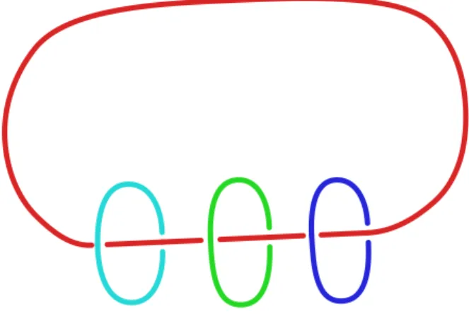
where Cg is a known prefactor given in [38]. Actually, (2.1) can be derived in various ways, either in the realm of LMO or of TQFT. Seifert spaces turn out to be tractable either because they can be obtained by rational surgery on a very simple link in S3(see Figure1), and TQFT behaves well under

surgery ; or because they carry a U p1q action and localization of the path integral occurs. Here is a schematic account of the history of those exact formulae:

‚ For g “ sup2q or sop3q and M a Seifert integer homology sphere, Lawrence and Rozansky [36] have used the Reshetikhin-Turaev construction to rewrite Z_CSg as a 1-dimensional integral (2.1), including contributions of all flat connections.

‚ Mari˜no generalized their derivation to any simply laced-Lie algebra g and Seifert rational ho-mology spheres M [38].

‚ Bar-Natan [4] has computed the LMO invariant of Seifert rational homology spheres, via the Kontsevich integral.

‚ Beasley and Witten [6] have developed a non-abelian localization method, allowing the com-putation of the contribution of isolated flat connections10 _{Then, correlation functions of Schur}

polynomials for the measure (2.1) can be interpreted in terms of Wilson loops along exceptional fibers [5].

‚ K¨allen [32] derives the same results, building on earlier work of [33] on a supersymmetric version of Chern-Simons theory.

‚ Blau and Thompson developed a diagonalization technique, first for U p1q bundles over smooth surfaces [9], then for U p1q bundles over orbifolds [10], allowing the computation of the full Chern-Simons partition function. As a particular case, they retrieve the earlier results on Seifert rational homology spheres.

4.4

Correlators and Wilson loops

We review the interpretation of the correlators of the model (2.1) in terms of Wilson loops. [5] tells us that the holonomy operator Uam along the exceptional fiber of order am– on the Chern-Simons side

– gets identified with diagpet1{am_{, . . . , e}tN{am_{q “ S}a{am _{– on the matrix model side, with the notations}

of (2.1). Therefore, the Wilson loop in representation R is equal to:

HR;am “ µ“chRpS

a{amq‰, _{S “ diagpe}t1{a_{, . . . , e}tn{a_{q, (4.15)}

where chR is the character of R, i.e. the Schur polynomial indexed by R. We prefer to work in the

power-sum basis of the representation ring, and with connected observables: Wn `k1 d1, . . . , kn dn ˘ “@Tr Uk1 d1 ¨ ¨ ¨ Tr U kn dn D conn “ µ“Tr S k1a{d1 _{¨ ¨ ¨ Tr S}kna{dn‰ conn,

10_{The trivial flat connection in a Seifert fibered spaces is isolated iff the a}

iare pairwise coprime. If χ ě 0, the only cases concerned are the lens spaces Lpp, qq, and the p2, 3, 5q cases including the Poincar´e sphere.

Figure 1: Seifert spaces which are rational homology spheres can be realized by rational surgery on this link with pr ` 1q components (here r “ 3). The surgery data is 1{b on the horizontal component and am{bm on the m-th vertical components (1 ď m ď r). Snappy courtesy of S. Garoufalidis.

where:

dj P ta1, . . . , aru, kjP Z`. (4.16)

The H’s and the W’s are related by a change of basis: to extract HR for a representation R

corre-sponding to a Young diagram with less n rows, we need to compute Wn1 with n1ď n.

Recalling a “ lcmpa1, . . . , arq, we define the n-point correlators of the matrix model as:

Wnpx1, . . . , xnq “ µ ” Tr x1 x1´ S ¨ ¨ ¨ Tr xn xn´ S ı conn “ ÿ l1,...,lrě0 µ“Tr Sl1_{¨ ¨ ¨ Tr S}ln‰ conn xl1 1 ¨ ¨ ¨ x ln n (4.17)

so that the Wn’s can be read from the coefficients of the expansion of Wnpx1, . . . , xnq in Laurent series

when x1, . . . , xn Ñ 8. If a1, . . . , ar are not coprime, the expansion of Wn also records expectation

values of fractional powers of the holonomy along fibers, which do not have a clear interpretation in knot theory.

In a perturbative expansion, we have a decomposition of formal power series in u of the form: Wnpx1, . . . , xnq “ ÿ gě0 N2´2g´nWpgq n px1, . . . , xnq, WnpgqP Qrrx ´1 1 , . . . , x´1n , uss (4.18)

Later, we shall consider only certain linear combinations of rotations of Wnpgq, namely:

´_ân i“1 ˆ vi ¯ ¨ Wnpgqpx1, . . . , xnq “ ÿ j1,...,jnPZa ˆ vpj1q ¨ ¨ ¨ ˆvpjnq Wnpgqpζaj1x1, . . . , ζajnxnq (4.19)

for ˆvi in a certain set V of vectors in Za. If we denote the discrete Fourier transform:

Fkrˆvs “

ÿ

jPZa

ζ_ajkvpjqˆ (4.20)

we have the expansions when xiÑ 8:

´_ân i“1 ˆ vi ¯ ¨ Wnpgqpx1, . . . , xnq “ ÿ k1,...,kně0 n ź i“1 Fkirˆvis xki i xTr Uk1 ¨ ¨ ¨ Tr UknDpgq conn (4.21) and when x Ñ 0: ´_ân i“1 ˆ vi ¯ ¨ Wnpgqpx1, . . . , xnq “ p´1qn ÿ k1,...,kně0 n ź i“1 Fki`1rˆvis xki`1 i xTr Uk1_{¨ ¨ ¨ Tr U}knDpgq conn (4.22)