Unemployment duration, city size, and the thightness of the labor market

HAL Id: hal-01462632

https://hal.archives-ouvertes.fr/hal-01462632

Submitted on 6 Jun 2020

HAL is a multi-disciplinary open access

archive for the deposit and dissemination of sci-entific research documents, whether they are pub-lished or not. The documents may come from teaching and research institutions in France or abroad, or from public or private research centers.

L’archive ouverte pluridisciplinaire HAL, est destinée au dépôt et à la diffusion de documents scientifiques de niveau recherche, publiés ou non, émanant des établissements d’enseignement et de recherche français ou étrangers, des laboratoires publics ou privés.

the labor market

Cécile Détang-Dessendre, Carl Gaigné

To cite this version:

Cécile Détang-Dessendre, Carl Gaigné. Unemployment duration, city size, and the thightness of the labor market. [University works] auto-saisine. 2009, 34 p. �hal-01462632�

Unemployment duration, city size,

and the tightness of the labor market

Cécile DÉTANG-DESSENDRE, Carl GAIGNÉ

Working Paper SMART – LERECO N°09-04

Unemployment duration, city size, and the tightness of the labor market

Carl GAIGNÉ

INRA, UMR1302 SMART, F-35000 Rennes, France Agrocampus Ouest, UMR1302 SMART, F-35000 Rennes, France

Cécile DÉTANG-DESSENDRE

INRA, ENESAD, UMR1041 CESAER, F-21000 Dijon, France

Acknowledgements

We are grateful to Daniel McMillen as well as Andrew Plantinga, Muriel Roger, Stuart Rosenthal, Harris Selod and Yves Zénou and for constructive suggestions. We also thank Mohamed Hilal and Virginie Piguet for their help to compute indexes.

Auteur pour la correspondance / Corresponding author Carl GAIGNÉ

INRA, UMR SMART

4 allée Adolphe Bobierre, CS 61103 35011 Rennes cedex, France

Email: Carl.Gaigne@rennes.inra.fr Téléphone / Phone: +33 (0)2 23 48 56 08 Fax: +33 (0)2 23 48 53 80

Unemployment duration, city size, and the tightness of the labor market

Abstract

This paper attempts to determine whether residential location affects unemployment duration. Our analysis is based on a spatial job search framework that shows the importance of dissociating the role of travel time from physical distance in unemployment duration. The contribution of our study also stems from the development of skill-specific accessibility measures that take into account the spatial distribution of labor supply and demand. Our results show that physical distance and competition among searchers must be controlled for in order to understand the significant role of job access (measured in terms of travel time) in unemployment duration. Second, improvements in access raise the probability that persons living in urban fringes and rural areas will become employed. Third, for workers living in large urban centers, the relationship between location and unemployment duration is insignificant.

Keywords: unemployment duration, job accessibility, commuting time JEL Classification: J64, R23

Durée de chômage, taille des villes, et accessibilité aux emplois

Résumé

Ce papier vise à déterminer si la localisation résidentielle affecte la durée de chômage. Notre analyse est basée sur un modèle spatial de recherche d’emploi mettant en avant l’importance de dissocier le rôle des trajets domicile/travail et de la distance physique dans la durée de chômage. La contribution de notre analyse réside également dans la construction d’indices d’accessibilité par catégorie socio-professionnelle prenant en compte la distribution spatiale de la demande et de l’offre de travail. Nos résultats montrent que l’accessibilité aux emplois (mesurée sur la base des temps de trajets) joue un rôle significatif dans la durée de chômage à condition que la distance physique et la concurrence entre rechercheurs d’emploi soient contrôlées. Ensuite, une amélioration de l’accessibilité accroit la probabilité de trouver un emploi pour les personnes vivant dans les zones périurbaines et les territoires ruraux. Enfin,

pour les travailleurs résidant dans les grandes agglomérations, la localisation résidentielle ne semble pas affecter la durée de chômage.

Mots-clefs : durée de chômage, accessibilité aux emplois, temps de trajet Classification JEL : J64, R23

Unemployment duration, city size, and the tightness of the labor market

1. Introduction

The effects of the spatial distribution of employment opportunities on unemployment duration have received much attention (see Gobillon et al., 2007 or Ihlanfeldt, 2006, for a recent survey). According to urban economists, the distance to jobs is a major factor in explaining adverse labor market outcomes (see Zénou, 2009). Recent studies in the spatial job search literature have shown how distance or travel time to jobs can reduce the probability of leaving unemployment (see for example Rouwendal, 1998 and Wasmer and Zénou, 2002.)1. Workers may refuse a job because commuting to it would be too costly in time or monetary terms in comparison with the wage offered. Among empirical studies, few papers have tested spatial models of job search (Patacchini and Zénou, 2006; Rogers, 1997; Rouwendal, 1999; Van Den Berg and Gorter, 1997).

In this paper, we provide a new empirical investigation of the role of residential location in unemployment duration, working with a French survey of workers located in different spatial categories (large urban centers, medium urban centers, urban fringe, and rural areas). Our approach is innovative in two ways. First, we recognize that physical distance and travel time are not perfectly correlated as the degree of congestion varies according to the location. For a given travel time, the physical distance should be lower in big cities than in rural areas, thereby increasing the reservation wage. As such, we control for both dimensions simultaneously in our study. Second, we propose an accessibility measure that takes into account the competition between workers for jobs, in order to reflect the tightness of labor market. Our accessibility measure varies by a worker’s skill level. Very few previous empirical studies allow for geographical variation in labor supply (Gurmu et al., 2008, Johnson, 2006, and Mattsson and Weibull, 1981, are exceptions) and none account for variation by skill.

Hence, the contribution of our paper is to test the role of residential location in unemployment duration by taking into account travel time and physical distance to jobs as well as the spatial structure of labor demand and supply. We also check whether the effect of the tightness of the labor market varies with respect to the city size. In France, the ratio of jobs to workers is

higher than one in big cities and lower than one in suburbs and remote areas. Furthermore, although jobs may be more plentiful in large cities, the probability of receiving a job offer may be higher in medium or smaller cities due to the lower number of job-searchers. This issue is particularly important because of its policy implications. As mentioned by Ihlanfeldt and Sjoquist (1998, p. 881), if the effects of residential location on unemployment vary by location, then the programs designed to mitigate the adverse labor market outcomes of commuting distance (such as car-pooling programs in US, or the French “prime transport” program currently under discussion) should target only to those cities where access to jobs plays a significant role.

We use individual data obtained from a French stratified survey (FQP: Formation, Qualification Professionnelle – Education, Professional Qualification) performed by the French National Institute of Economic Statistics.2 Workers in our sample are located in different types of urban and rural areas. For each individual, the survey provides information on their job status in 1998, in 2003, their monthly progress in the labor market between these dates, their location at the municipality level and other economic and social characteristics. Our methodological approach is to estimate unemployment duration models with a piecewise constant hazard specification and unobserved heterogeneity, while addressing potential endogeneity problems.

The main results are as follows. First, we show that physical distance and competition among searchers must be controlled for in order to estimate the effects on unemployment duration of accessibility to jobs (measured in terms of travel time). As emphasized by Ihlanfeldt and Sjoquist (1998), precise of measures of job accessibility are needed to reveal the negative relationship between access to jobs and the probability of leaving unemployment. Second, our analysis suggests that job accessibility plays a significant role in unemployment duration for workers living in rural areas and in urban fringes. Although the probability of finding a job increases with job accessibility in large cities, the correlation is not significant. Robustness checks confirm the main findings.

In the next section, we develop a spatial job search model in order to show how distance and travel time affect unemployment duration. In section 3, we present our accessibility index.

2Very few empirical studies have been carried out in Europe on the relationship between residential location and

Section 4 is devoted to the presentation of the French survey data as well as employment and labor force data at the municipality level. Section 5 presents the estimation strategy and the results. The last section concludes.

2. Theory

In this section, we specify how the spatial structure of local labor markets influences the individual’s ability to find employment. We develop a spatial version of a job search model, by considering both time travel and distance in the framework in Rouwendal (1999). The instantaneous utility function experienced by a worker living in a municipality is given by:

( ) ( )

u v w d h d (1)

where w is the wage rate at his/her workplace,  means the transport cost per distance unit, dis the physical distance between his/her workplace and his/her residential municipality,  stands for the disutility arising from commuting time h depending positively on the distance.3 The preferences are additive in the wage net of commuting cost and in commuting time. The first component (.)v encapsulates the pecuniary aspects of the job offer (including the commuting costs) while the last component h d( )reflects the non pecuniary aspects of commuting. We assume that the relationship between h and d is given by

hd (2)

Parameter  means the degree of congestion or the average trip speed around the worker’s residential location. The higher  is, the higher the degree of congestion.4

If the worker is unemployed, the instantaneous utility reaches the following value:

u b (3)

where b is the net benefit of search costs received by unemployed workers. We neglect search costs related to distance. We know from the job search theory that a rise in search costs

3_{We do not take into account the fact that commuting time may reduce welfare through a labor-leisure choice,}

which implies that a unit of commuting time is valued at the wage rate (Fujita, 1989, ch. 2). Such a model is cumbersome to analyze and is beyond the scope of our paper.

4 _{Patacchini and Zénou (2005) use the same assumption to take into account the impact of different transport}

modes on search effort. However, the authors do not control for both physical distance and travel time in their econometric analysis.

implies a decrease in the reservation wage, thereby increasing the probability of finding a job (Lippman and McCall, 1976). Consequently, by considering that distance does not significantly influence search costs, we assume that the distance to the job center does not influence unemployment duration by this channel.

Job offers arrive at random intervals at a constant arrival rate  which is specific to the worker’s residential location. This probability of receiving a job offer for a searcher varies across space with   , where [0,1] is non-spatial friction depending on individual characteristics, whereas  is the job availability facing a searcher and is a function of the spatial distribution of vacancies and other searchers surrounding his/her place of residence. In line with Rouwendal (1999), a job offer at time t is a random drawing without recall from a simultaneous probability density function f w d of wage rates and commuting distance. ( , ) The jobs are evaluated by means of the utility function given by (1). Hence the density function _{f u of the utilities from jobs that are offered is given by} *_{( )}

*_{( ) ( , )d d} f u f w d w d u   



(4)

Equation (4) transforms the simultaneous density of wage rates and commuting distances into a one-dimensional density of utilities of supplied jobs.

As in traditional job search theory, job searchers maximize their own expected present value of utility over an infinite horizon. Utility is intertemporally separable. In accordance with our data, we assume that job searchers do not change residence (90% of the sample of unemployed individuals lived in the same municipality throughout the search period). The optimal strategy is as follows. There is a utility threshold value u and the first job offer leading to utility higher than u is accepted. Formally, reservation utility u is implicitly given by the following equality:

* ( ) ( )d u u b  u u f u u    



 (5)

where  is the rate of discount. By using (4), (5) can be rewritten as follows:

[ ( , ) ] ( , )d d   _  



 u u u b u w d u f w d w d (6)

Hence, the reservation utility property of the optimal search strategy considered implies that a minimum wage rate exists, defined by w , such that

( , )

u u w d (7)

By introducing (7) in (6) it is straightforward to check that: d ' ' 0 d u w w h u u h u u d d h d d h d                _{}  

with u'   u/ w 0 and    h d  0. Therefore, the impact of commuting time on the reservation wage is given by

1 ' 0 2 ' w u h u       _{  }    _{ } (8)

Hence w h/ 0 so that commuting time raises unemployment duration. There is a tradeoff between additional commuting time and higher wages. In other words, compensation is required for commuting. Such a result is obtained by Rouwendal (1999). However, our analysis also reveals that the impact of commuting time on the reservation wage increases with commuting costs  and decreases with the degree of congestion . As expected, wages must compensate commuting costs.

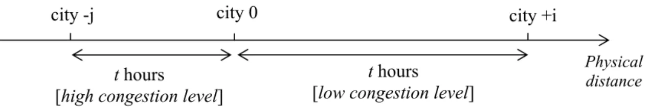
More surprisingly, congestion in transportation affects the reservation wage negatively, for a given time distance. To illustrate this result, let us consider a region described by a one-dimensional space where all jobs are located on the same city (say city 0), as shown in Figure 1. It is assumed that cities located on the right-hand side of city 0 are connected by a smooth motorway while cities located on the left-hand side of city 0 are connected by a crowded road network. In this case, two individuals located in either side of the city at the same time distance (t hours) to jobs do not cover the same physical distance because congestion is different in both sides. More precisely, as shown in Figure 1, a person located in the right-hand side (in city +i) must pay more commuting costs (in pecuniary terms) than a worker living in the left-hand side (in city –j). Hence not all workers located at the same time-distance necessarily incur the same commuting costs. As a result, our estimations must control for the physical distance to jobs to isolate the effect of commuting costs on unemployment duration.

Figure 1: Time travel and physical distance

3. Measuring accessibility

Rogers (1997) proposes an accessibility measure that accounts for the spatial structure of employment. Its index is the sum of the number of jobs weighted by the commuting time from residential location and workplace, within a commuting time of T-minutes from home. Cervero et al (1999) suggest introducing an empirically derived impedance coefficient for commuting trips and an element of “occupational matching” (i.e. weighting the employment in an occupational class k by the proportion of employed residents in zone i working in this class k). Gurmu et al. (2008) introduce separately a job access measure very similar to the Roger’s and a measure of competition labor supply, which is a distance-decay function of the labor supply living around the residential location.

In this paper, we improve these indexes by encapsulating both effects and also controlling for the disutility arising from commuting time. Additionally, our index varies by a worker’s skill level, because the spatial distribution of employment and the disutility arising from commuting time differ with respect to skill.

Hence the accessibility measurement for a worker endowed with a skill l living in a municipality r can be expressed as follows (Figure 2):





( ) exp l j l l r rj l rj j j L A h T h Q   



 where





( ) exp l l l j kj k kj k Q h T 



C  h city 0 _{city +i} city -j t hours [low congestion level]

Physical distance

t hours

with j being the municipalities within a radius of T minutes from r and l j

L the number of jobs of type l located in j, h the travel time from r to j following the road network while_{r j,} l

k C stands for the number of individuals of type l and located in k, belonging within a radius of T minutes from j. In addition, parameter_l _{expresses the marginal impact of commuting time} on workers’ utility by skill.

Figure 2: Accessibility index

Our measure of job accessibility reflects each worker’s proximity to jobs for which she or he is qualified, relative to the number of workers competing for these positions. When a person living in municipality i applies for a job located in municipality j, this person has to compete with all other applicants who can reach municipality j. Thus, we must divide jobs located in destination municipality j by the workers within reach of that municipality j. Hence, by introducing Q, we control for the potential competition among workers for a job located in j. This means that the probability of receiving a job offer with skill l located in j decreases also with the mass of workers living around this location.

T hrj T hkj municipality r municipalityj

Job access from r

Potential competitors for a job in j

4. Data and descriptive statistics 4.1. Databases

The main data set used is obtained from a French stratified survey of around 40,000 adults performed in 2003 by the French National Institute of Economic Statistics, the FQP sample (Formation, Qualification Professionnelle). For each individual, the survey provides information regarding their job situation in 1998, in 2003 and their labor market progress month by month between both dates. It also gives details on their initial and on-the-job training and on their social characteristics (gender, age, skill, household size, geographical origin, education). We work with a sub-sample of 2,888 individuals aged from 16 to 60 in 1998, who had a job in April 1998 and entered unemployment between April 1998 and December 2002. The selected workers are located in different municipalities belonging to different spatial categories (rural areas, urban fringe, small cities and large cities).

In addition, by selecting only claimants having already worked, we are able to identify their skill to consider an index of accessibility to jobs corresponding to them5_{. We distinguish} skilled manual workers, unskilled manual workers, clerks and executives. Knowing their job status (employed, unemployed, inactivity, training) month by month, we can piece together unemployment durations of at least one month. Note that we work on individual declarations and not on administrative registration of unemployment. We focus our analysis on the first period of unemployment registered after 1998, as available information on job qualification only concerns occupied jobs in 1998 and in 2003. Note that 22.7% of individuals in our sample experienced more than one spell of unemployment during the observed period. Among the 2,888 spells analyzed, 11.5% are right censured. Individual characteristics include gender, age and children or no children at the beginning of unemployment duration6, qualification of the last job and ethnic origin. To control for individual dynamism in job searching, we introduce a dummy variable equal to one if the individual has voluntarily quitted one’s job over the last 5 years.

5 _{It is implicitly assumed that individuals search for a job whose skill is comparable to their previous one.}

6 _{Marital status is not introduced as only official weddings are known whereas nothing is known about}

The mean of unemployment duration in our sample is 12.2 months and the median is 8 months. From Kaplan-Meier statistics, it can be concluded that the probability of still being unemployed after 9 months is around 50% (Figures 3a and 3b). The individual characteristics are summarized in Table 1. The majority of individuals are clerks. Average unemployed duration of men is significantly lower than that of women (10.6 vs. 13.7 months). Individuals aged over 50 stay an average of 1.5 month longer in unemployment than younger workers (12 vs. 13.5 months). Executive and skilled manual workers spend an average of 11 months in unemployment while this figure is 13 months for unskilled manual workers and clerks. The individuals of African origin remain in unemployment for an average of 1.5 months longer than other categories.

Figure 3a: Kaplan-Meier survival estimate Figure 3b: Distribution

0. 00 0. 2 5 0. 50 0. 75 1. 0 0 0 10 20 30 40 50 analysis time

Kaplan-Meier survival estimate

0 10 0 20 0 30 0 F req ue nc y 0 10 20 30 40 50 dchomc

Table 1: Individual characteristics, descriptive statistics

Variable % or mean

Gender (man) 46.5

Having children(a) _39.3

Age(a) _{34.6 years}

African origin(b) _9.2

On the job search in the last 5 years 32.4

Skill:

Unskilled manual worker Skilled manual worker Clerk Executive 19.2 15.9 44.7 20.2 Residential location: Urban centers Urban fringe Rural area 61.45 20.45 18.20 (a) at the beginning of the unemployment spell (b) Maghreb and other African countries

4.2. Spatial categories and spatial variables

The location of each individual in the sample is known at the municipality level. The municipality is the lowest French administrative scale. Mainland France includes 36,565 municipalities that are divided in three main categories: (1) urban centers with 5,000 jobs and more, (2) urban fringe concerns all communes where at least 40% of the resident population work in an urban center, (3) rural areas encompass all other municipalities (Map 1 in Appendix A). Among urban centers, we distinguish big central cities with more than 150,000 inhabitants from others. Each municipality belongs exclusively to one of four spatial categories. Urban centers concentrate 60% of the French population and 20% are in urban fringe. The other workers reside in rural areas (all other municipalities). As shown by Table 1, the spatial distribution of individuals in our sample reflects the spatial distribution of the French population.

We can thus calculate the accessibility index for each municipality.7 We require data for potential vacancies, potential searchers, travel time between each pair of municipalities and a proxy for the disutility arising from commuting. Measuring the available jobs for which an individual is qualified with a high degree of precision represents a considerable challenge. To measure job opportunities, Johnson (2006) uses the numbers of recently filled jobs and net hires (job opportunities generated by employment growth), whereas Kawabata and Shen (2006) consider job opportunities generated by employment growth and by turnover. As this information is not available to us, we use the total number of jobs within a given commuting area8. To approximate these two components, the National Census of 1999 provides the number of workers by municipality and by skill as well as the number of jobs (because we know the location of the workplace for each worker) by location and skill. Note that the surface of municipalities is relatively low in France. The median surface is 10.72 km² and 75% of municipalities have a surface lower than 18.3 km² 9_{. Thus, intra-municipality distance} is small in the great majority of cases and can be neglected. The consequences of this choice are discussed thereafter.

The evaluation of travel time between two municipalities is based on a road network encapsulating all French municipalities (Hilal, 2004), considering distance, type of road, traffic speed and specific traffic conditions (urban, mountain areas...).

We have evaluated the marginal impact of commuting time on individual utility level () using a gravity framework. The journey-to-work flows between two locations are considered as a function of employment and population sizes, distance and cost to overcoming this distance (captured by ). This estimated distance decay function encapsulates the composite effects of commuting time in reducing the probability of searching for, finding and accepting distant job offers. As Johnson (2006, p. 343) argues, it discounts distant employment opportunities as well as distant competing workers. As estimation of a gravity model with more than 36,000 locations cannot be considered, we use aggregate data and assume that the relationship between the flow level and the commuting time reflects this discount parameter. The National Census of 1999 gives commuting flows by skill at the municipality level and the distribution of commuting time between the centroid of municipalities. No account is taken of

7 _{Except for Paris, Lyon and Marseille which are divided respectively in 20, 9 and 16 “arrondissements”.} 8 _{As in Rogers (1997) and Gobillon and Selod (2006).}

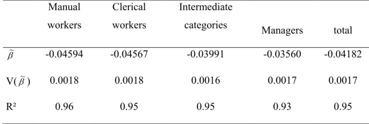
time-distances greater than 150 minutes as they correspond to weekly commutes. Around 40% of commutes are intra municipality (i.e. their commuting times are assumed to be null). Thus commuting time is underestimated, especially in the case of cities with a large area. We tested different specifications to link the volume of flux and commuting time. The negative exponential gives the best fit. The estimates obtained are summarized in Table 2. The time-distance deterrence coefficients  are close to those obtained by Johnson (2006) from a gravity model using US data. In addition,  decreases with skill level, in accordance with the findings obtained by Johnson. Note also that Van den Berg and Gorter (1997), who estimate the disutility from commuting directly, show that the coefficient decreases with the level of education. Using our estimated disutility parameter for manual workers, nearby jobs (competing workers) are weighted more than distant ones: jobs located at 15, 30, 45 and 60 minutes would have weights of 0.50, 0.25, 0.13 and 0.0610_.

Table 2: Estimated value for ~by skill ( ,

, r j h r j r flow L e  )  Manual workers Clerical workers Intermediate

categories _{Managers total}

~ -0.04594 -0.04567 -0.03991 -0.03560 -0.04182

V(~) 0.0018 0.0018 0.0016 0.0017 0.0017

R² 0.96 0.95 0.95 0.93 0.95

4.3. Descriptive statistics on accessibility indexes

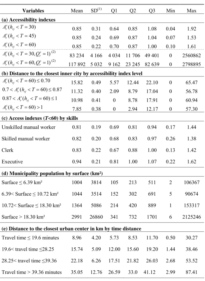
In this subsection, we show that (i) increasing the commuting time interval reduces the dispersion of values provided by accessibility measurements; (ii) distances to the closest part of the inner city vary greatly for the same accessibility (defined in travel time), (iii) the accessibility measure varies with respect to skill.

Table 3 reveals that increasing the commuting time interval reduces the dispersion of values of the accessibility index. Indeed, the employment/population ratio is higher than one in the

central city and decreases with distance to them to reach a value inferior to one in small municipalities. Hence, when the maximum commuting time T is short enough, the access measurement of small cities does not include employment located in the city center and underestimate job opportunities and accessibility level in these small municipalities. In contrast, for city center, the index with T short overestimates the accessibility level, as it does not consider workers living in their periphery. Increasing T leads to a smoothed index (see Map 2 and 3 in Appendix A), given a more realistic view of job accessibility.

We also evaluate the mean distance to the closest inner city for four groups of workers according to their accessibility indexes: individuals whose accessibility index is inferior to the first quartile, between the first and second quartile, and so on. The results in Table 3 reveal that high accessibility values imply a residential location close to the central city. 48% of individuals being in the 4th quartile of the accessibility index (higher than one), live in a center of an urban area as opposed to 28% in the whole sample. However, the dispersion within each interval remains large even in the fourth quartile. Indeed, among individuals belonging to the fourth quartile, 25% of individuals live in a municipality located at more than 12 km from the closest city center. In addition, the gap between the first and the third quartile (Q3-Q1) increases from 12 to 17 km when the access measurement decreases. In other words, potential commuting costs can vary significantly for individuals with similar job accessibility.

Finally, the higher the skill, the higher the accessibility index. Hence, even though a control is performed for the spatial distribution of labor supply, it can be seen that low skill workers reside far from job opportunities.

Table 3: Spatial variables, descriptive statistics

Variables Mean SD(1) Q1 Q2 Q3 Min Max (a) Accessibility indexes

( 30) s r rj A h  T _{0.85 0.31 0.64 0.85 1.08 0.04 1.92} ( 45) s r rj A h  T _{0.85 0.24 0.69 0.87 1.04 0.07 1.53} ( 60) s r rj A h  T _{0.85 0.22 0.70 0.87 1.00 0.10 1.61} ( 30, 1) s s r rj r A h  T Q  (2) 83 234 4 166 4 034 11 706 49 401 0 2560862 ( 60, 1) s s r rj r A h  T Q  (2) 117 892 5 032 9 162 23 245 82 639 0 2798895

(b) Distance to the closest inner city by accessibility index level

(  60) 0.70 s r rj A h T _{15.82 0.49 5.57 12.44 22.10 0 65.47} 0.7 s(  60) 0.87 r rj A h T _{11.32 0.40 2.09 8.79 17.04 0 56.78} 0.87 s(  60) 1 r rj A h T _{10.98 0.41 0 8.78 17.91 0 60.94} (  60) 1 s r rj A h T _{7.85 0.38 0 2.94 12.17 0 57.30}

(c) Access indexes (T<60) by skills

Unskilled manual worker 0.81 0.19 0.69 0.81 0.94 0.17 1.44

Skilled manual worker 0.82 0.20 0.68 0.83 0.97 0.26 1.38

Clerk 0.83 0.22 0.67 0.88 1.00 0.13 1.42

Executive 0.94 0.21 0.81 1.00 1.07 0.22 1.62

(d) Municipality population by surface (km²)

Surface ≤ 6.39 km² 1004 3814 105 213 511 2 106367

6.39< Surface ≤ 10.72 km² 1044 3514 152 302 691 5 90674

10.72< Surface ≤ 18.30 km² 1364 5086 214 420 889 1 153317

Surface > 18.30 km² 2991 26860 341 732 1701 6 2125246

(e) Distance to the closest urban center in km by time distance

Travel time ≤ 19.6 minutes 8.96 4.20 5.73 8.53 11.70 0.50 30.27

19.6< travel time ≤28.25 15.74 5.09 12.00 15.60 19.20 1.44 38.46

28.25< travel time ≤39.36 22.18 6.26 17.51 21.82 26.03 2.68 53.52 Travel time > 39.36 minutes 35.05 12.76 26.59 33.0 41.12 2.99 87.41

5. Empirical investigation 5.1. The empirical model

To capture the impact of the local labor market structure on unemployment, we estimate duration models with a piecewise constant hazard specification and unobserved heterogeneity. Durations are modeled in terms of the hazard function 

 

t or instantaneous rate of occurrence of the event (exit from unemployment) given that it has not occurred before:

 





0 Pr | lim dt t t t dt t t t dt       

A central issue is the duration dependence (i.e. the impact of the length of the spell on the hazard function). So as not to specify a functional form for the baseline hazard, time is subdivided into intervals and it is assumed that the baseline hazard is constant in each interval (Lancaster, 1990). Thus, we consider _ij _jexp

 

x_i where _ij is the hazard for individual i in interval j, _j is the baseline hazard for interval j, and exp{x_i is the relative risk for an } individual with covariate values x_ij, compared to the baseline at any given time. Note that with a logarithmic form, we obtain a log-linear model.11

We allow for unobserved individual-level heterogeneity by introducing an additional unmeasured covariate (a frailty) following a gamma distribution with parameter θ. The piecewise constant hazard model with unobserved heterogeneity is a tractable empirical approach for controlling the problem of bias due to negative time dependence. Indeed, part of the time dependence due to state dependence (decreased probability of finding a job as a function of the time spent in unemployment since the long-term unemployed receive fewer job offers) is captured by the estimation of a piecewise constant baseline hazard. Moreover, part of the time dependence due to unobserved individual characteristics (decreased probability of finding a job as a function of the time spent in unemployment, as the long-term unemployed have unfavorable characteristics and weak employability) is captured by frailty.

The period observed from 1998 to 2002 corresponds to a prosperous and homogeneous period for unemployment and for job creation in France (following a slow-growth period from 1993 to 1997 and followed by another period with few job creations from 2002 to 2005). A test was performed to identify a conjuncture effect though none was found.

In addition, the estimated effects of job accessibility might suffer from omitted variable bias. In order to reduce this bias, we control for neighborhood characteristics. Because the measures of job accessibility may simply capture spatial differences in employment structure, we introduce a set of controls for spatial variables in the estimations. We include the prevailing unemployment rate in the labor market area as well as two measures of local economic structure. Because we select individuals who have already worked, we observe the economic sector in which individuals obtained a job. Hence, we develop a local specialization index equal to the share of total employment belonging to the sector in which the individual worked. We also construct a local sectoral diversity index using a Herfindhal index. The sectoral classification that we use disaggregates employment into 16 sectors.

Finally, because our sample includes only those who are working at the start of the period and most of them (90%) do not move throughout the search period, we can assume that job search results are observed for a fixed residential location. The choice of housing location is more likely to be related to the location of the previous job than to be contemporaneous with job search. This endogeneity issue is addressed more precisely below.

5.2. Empirical results

We first consider the effects of workers’ individual characteristics. The time dependence of the hazard is non-linear12 and θ is significant at the 5% to 8% level, depending on the model, thus revealing weak unobserved individual heterogeneity. The coefficients on the individual variables have the expected signs and do not significantly change with the labor market characteristics (see Models I to IV in Table 4). As shown in numerous empirical studies (Aznat et al., 2006), unemployment duration is larger for women with young dependent children. The hierarchy along the skill scale is also well known: unskilled manual workers stay unemployed the longest, followed by clerks, skilled manual workers and then executives.

As in other studies, ageing has a negative impact on the duration of unemployment13. Individuals of African origin stay unemployed longer than others, a situation observed in other developed countries14.

Role of travel time, distance and competition. In what follows, we discuss the importance of travel time, physical distance and competition between job-seekers in the analysis of the residential location effect on unemployment duration. First, alternative measures of access have no significant impacts on unemployment duration when the commuting time maximums are T= 30 or 45 minutes. The over (under) estimation of job opportunities in large (small) municipalities (see section 4.3 and Maps 2 and 3 in Appendix A) when T is small leads to a blurred view of the relation between accessibility and unemployment duration.

The results in Table 4 and the table in Appendix B allow us to conclude that proximity to jobs has a significant impact provided that one controls for competition among searcher. Without this control, we find no significant impact of proximity to jobs on the probability of leaving unemployment (see Appendix B). This result confirms that living in a municipality with a high local labor demand does not induce a higher probability of leaving unemployment. What matters is the ratio between potential jobs and potential job searchers.

In addition, introducing the physical distance to the closest city center improves the precision with which we measure the relationship between access and unemployment duration. In Model III in Table 4, the coefficients associated with our access measure are more significant. However, when we compare Model II and III in Table 4, we find that taking into account the role of physical distance in the job search strategy, in addition to travel time, provides only slight improvements.

13 _{Alba-Ramirez et al. (2007) find a nonlinear relation suggesting that the first entrance in the labor market can}

generate a long unemployment duration. When considering only individuals with at least one job experience, we find a consistent linear relation between age and unemployment duration.

14 _{There is a great deal of literature on this subject, particularly in the US, but also in OECD countries (see for}

example the special issue of the Journal of Population Economics, e.g. Card and Schmidt, 2003). The relatively limited effect observed in our study comes from the selected sample. When selecting unemployed with job experience, the impact of ethnic origin proves limited. Additional investigations on another sample would be useful to study this subject in greater depth.

Table 4: Results (dependent variable: unemployment duration)

Model I Model II Model III Model IV

Variables estimates estimates estimates estimates

Gender (ref: woman) 0.088 0.087 0.087 0.097

0.060 0.060 0.060 0.060

Female with children <16 yearsa _{-0.299*** -0.302*** -0.307*** -0.312***}

0.056 0.054 0.057 0.057 Male with children <16 yearsa _{-0.054 -0.054 -0.056 -0.054}

0.612 0.614 0.614 0.614 Skilled MW (ref: unskilled MW) 0.157** 0.150** 0.150** 0.135**

0.068 0.068 0.068 0.068

Clerk (ref: unskilled MW) 0.118** 0.117** 0.119** 0.136**

0.053 0.054 0.054 0.054 Executive (ref: unskilled MW) 0.205*** 0.235*** 0.237*** 0.247***

0.063 0.065 0.065 0.065

Age -0.013*** -0.014*** -0.014*** -0.013***

0.002 0.002 0.002 0.002

African origin -0.137* -0.133* -0.130 -0.115

0.082 0.083 0.083 0.083

Voluntary job change in the last 5 years 0.163*** 0.158*** 0.158*** 0.146***

0.045 0.045 0.045 0.045

Access index (T<60) 0.910* 0.961* 1.043**

0.547 0.549 0.335

Access index squared -0.641* -0.658** -0.715**

0.333 0.321 0.336

Dist to closest inner city 0.001 0.001

0.001 0.001

Local unemployment rate -0.015**

0.006

Local specialization index 0.041*

0.022

Local Herfindhal index -3.448**

1.706

Log likelihood -3690 -3669 -3669 -3630

Number of observations 2888 2888 2888 2888

Piecewise baseline hazards are not reported. Standard errors are in italics. a: the reference is workers with no children). MW means manual worker.

Last, when we introduce control variables for local economic conditions (local unemployment, the specialization index and the Herfindhal index), coefficients associated with the access measure have the same magnitude but are more significant (see model IV in Table 4). The estimated effects of job accessibility weighted by potential competition among searchers do not seem to suffer from bias due to omitted neighborhood characteristics. As expected, a high unemployment rate prevailing in the local labor market reduces the probability of finding a job. Conversely, unemployment duration diminishes when the unemployed worker resides in a region specialized in the sector in which she previously worked. Nevertheless, this relationship needs more investigation because this effect can depend on the local growth rate of sectoral employment. A negative relationship is found between the probability of leaving unemployment and the index of local sectoral diversity. A complete study of the impact of local economic structure on unemployment duration is required but is beyond the scope of our paper.

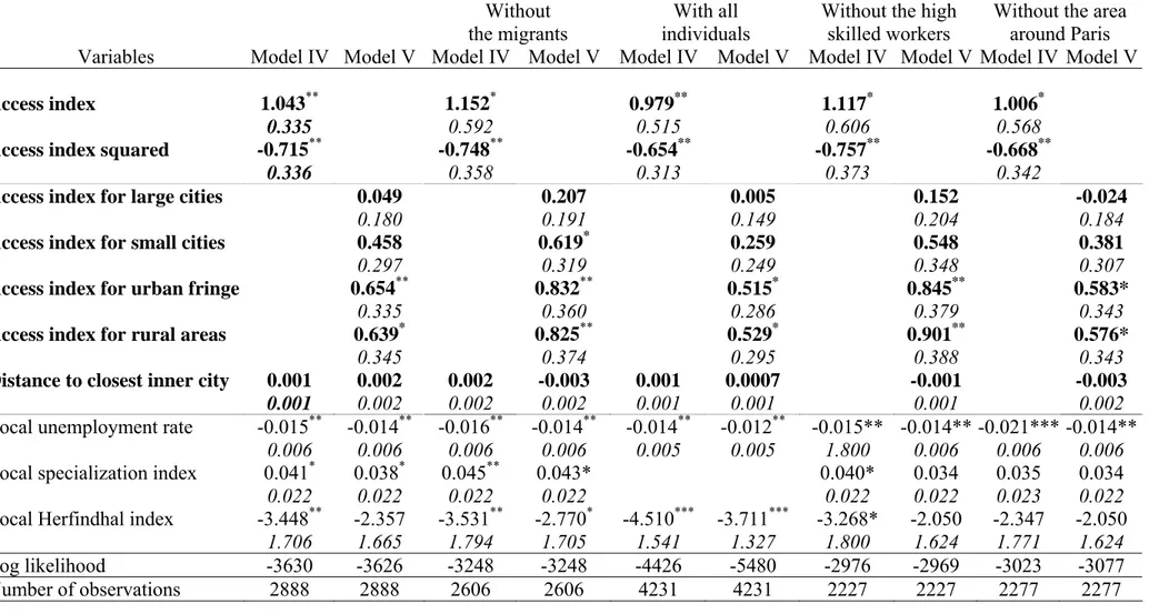
The role of job access by type of cities. The impact of job access on the probability of finding a job is non-linear (Models II-IV). In particular, the probability of leaving unemployment is greatest at the access index intermediate values. At very low or very high values, a rise in access to jobs induces only a slight improvement in unemployment duration. From Table 5, we can determine whether the residential location effect on unemployment duration differs according to the type of urban or rural area. We use the following classification of residential location: large central cities (with more than 150,000 people), other urban centers, municipalities located in urban fringes and rural areas. The relationship between unemployment duration and job access becomes insignificant for workers living in large urban centers and linear for the other workers. For workers living in urban fringe and rural areas centers, a rise in accessibility to jobs increases the probability of leaving unemployment.

Table 5: Additional results (dependent variable: unemployment duration)

Without the migrants

With all individuals

Without the high skilled workers

Without the area around Paris

Variables Model IV Model V Model IV Model V Model IV Model V Model IV Model V Model IV Model V

Access index 1.043** 1.152* 0.979** 1.117* 1.006*

0.335 0.592 0.515 0.606 0.568

Access index squared -0.715** -0.748** -0.654** -0.757** -0.668**

0.336 0.358 0.313 0.373 0.342

Access index for large cities 0.049 0.207 0.005 0.152 -0.024

0.180 0.191 0.149 0.204 0.184

Access index for small cities 0.458 0.619* 0.259 0.548 0.381

0.297 0.319 0.249 0.348 0.307

Access index for urban fringe 0.654** 0.832** 0.515* 0.845** 0.583*

0.335 0.360 0.286 0.379 0.343

Access index for rural areas 0.639* 0.825** 0.529* 0.901** 0.576*

0.345 0.374 0.295 0.388 0.343

Distance to closest inner city 0.001 0.002 0.002 -0.003 0.001 0.0007 -0.001 -0.003

0.001 0.002 0.002 0.002 0.001 0.001 0.001 0.002

Local unemployment rate -0.015** -0.014** -0.016** -0.014** -0.014** -0.012** -0.015** -0.014** -0.021*** -0.014**

0.006 0.006 0.006 0.006 0.005 0.005 1.800 0.006 0.006 0.006

Local specialization index 0.041* 0.038* 0.045** 0.043* 0.040* 0.034 0.035 0.034

0.022 0.022 0.022 0.022 0.022 0.022 0.023 0.022

Local Herfindhal index -3.448** -2.357 -3.531** -2.770* -4.510*** -3.711*** -3.268* -2.050 -2.347 -2.050

1.706 1.665 1.794 1.705 1.541 1.327 1.800 1.624 1.771 1.624

Log likelihood -3630 -3626 -3248 -3248 -4426 -5480 -2976 -2969 -3023 -3077

Number of observations 2888 2888 2606 2606 4231 4231 2227 2227 2277 2277

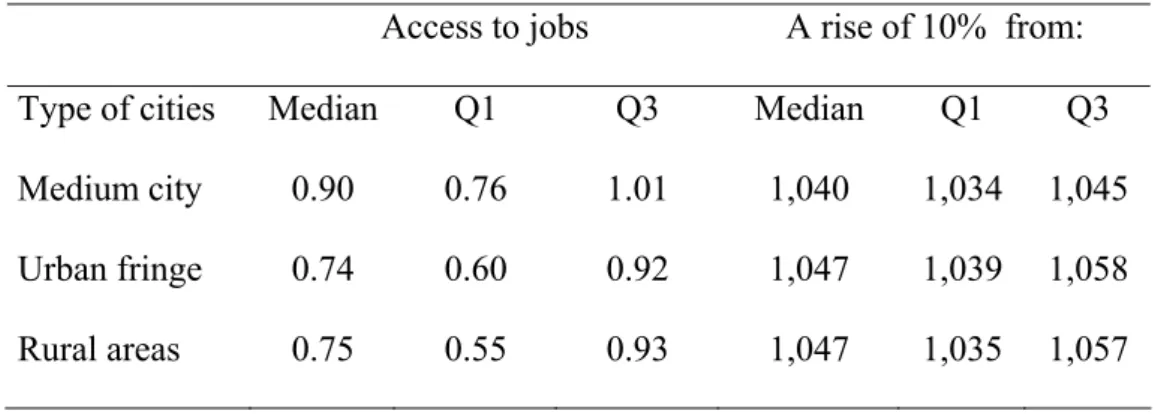
As shown in Table 6, a 10% rise in the accessibility index increases the probability of finding a job by 5% for a median worker living in urban fringe and rural areas. This marginal impact is slightly lower for workers living in medium cities. Hence our result differs greatly from that of Weinberg (2004), who finds that job accessibility has a weaker impact in small metropolitan areas than in large ones. However, this study does not control for the role of physical distance and travel time. When both variables are considered, job accessibility has a stronger impact on unemployment duration for workers living in medium and small municipalities. This implies that residential location far from large cities significantly reduces opportunities for finding a job. Such a result could justify on equity grounds regional policies in favor of rural or urban fringe areas.

Finally, we observe that the probability of finding a job is not affected by accessibility to jobs in the largest urban centers. This result could arise from the fact that our travel time variable does not identify the use of public transportation by workers living in very large cities. However, this result is in accordance with the findings of a study on Paris and its suburbs by Gobillon and Selod (2006). Even when public transportation is taken into account, they show that job accessibility is not a crucial factor for explaining unemployment duration. This result confirms the need for specific studies on the relationship between urban ghettos, unemployment and discrimination in studies of labor outcomes in large cities and emphasizes the limitations of a spatial job search approach that does not include housing segregation.

Table 6: Marginal impact of A_rs by type of space

Access to jobs A rise of 10% from:

Type of cities Median Q1 Q3 Median Q1 Q3

Medium city 0.90 0.76 1.01 1,040 1,034 1,045

Urban fringe 0.74 0.60 0.92 1,047 1,039 1,058

5.3. Robustness checks

Endogeneity issue. We now check the robustness of our results. Although our sample includes only the individuals having already worked and 90% of them do not move throughout the search period, there are some potential sources of endogeneity. First, the one-tenth of individuals who have changed their residential location may bias the results if those who move for a job are also those with the lowest measures of accessibility. To address this concern, we estimate models IV and V without individuals who moved during the search period. The results reported in Table 5 show that our findings hold and are more significant. Second, by restricting the sample to those individuals with a job at the beginning of the period, we may select the individuals who are likely to be the most employable. In such a case, the impact of job accessibility on unemployment duration is under-estimated. We perform an additional regression with the full sample of workers. As shown in Table 5, job access has a significant effect for the individuals living in rural areas and urban fringe, consistent with earlier findings. However, we have to be cautious about this comparison because of some differences with the previous estimations. In particular, we do not know the skill level of previously unemployed individuals and the job access measure uses all type of jobs and workers. Further, we cannot control for the sectoral specialization of the local labor market.

A third source of endogeneity is the spatial selection mechanism. The reasoning is as follows. (1) Suppose access level is positively correlated with the municipality size. (2) Further, assume that the most able and ambitious workers, those who have the highest probabilities of being employed and moving quickly out of unemployment, locate primarily in big city centers (Glaeser and Maré, 2001). (3) As it is difficult to control for an individual’s ability and ambition15, a correlation may be observed between access level and employment probability or unemployment duration that is just a consequence of selection bias. The question of neighborhood selection commonly arises in intra-metropolitan area tests: “Sorting of low labor attachment individuals into neighborhoods with worse job access biases these estimates up” (Weinberg, 2004, p506). Inter-metropolitan tests are confronted by firm location endogeneity: low labor attachment individuals concentrated in specific areas could discourage

15 _{We introduce an indication of dynamism with a dummy variable for voluntary on-the-job search during the 5}

firms from being located in these areas. In our case, we measure municipality level job accessibility over the entire French territory. The spatial distribution of the labor force on an urban-rural gradient exhibits an representation of executives in urban centers, an over-representation of blue collar workers in rural areas and an equal-over-representation of clerks (Huiban et al., 2004). There is no reason to suspect that one category has lower labor attachment than another. Nevertheless, we use the whole sample of individuals having a job in April 1998 to verify that the accessibility index and location in a city center can be treated as exogenous determinants of the probability of being unemployed at least one time between 1998 and 2002. For the accessibility index, a continuous variable, we perform a classical test based on the estimation of the complete model by maximum likelihood (Wooldridge, 2002). For the discrete variable, living in a city center, we use the test designed by Lollivier (2001)16. Exogeneity is accepted in both cases.

Additional results. Our estimations pool workers of different skills together so that we evaluate the average accessibility effect in France and by type of space, even though our access measure takes into account the spatial distribution of jobs and workers by skill. It would be interesting to study whether the impact of residential location on unemployment duration varies with skill level. Ideally, one would estimate separate models by skill groups. However, the number of individuals by skill group is too low to estimate separate models. Because location is expected to affect more strongly the labor market outcomes of less skilled workers, we estimate Models IV and V without the executives (this removes 661 individuals). Recall that these high skilled workers have, on average, the highest levels of job access (see Table 3(c)). The results are reported in Table 5 and show that the coefficients have the same magnitude but are more significant. A different database is required to check whether location acts as a barrier to employment for high skilled workers.

Finally, it is recognized in France that the labor market in the Paris area and its hinterland (Ile-de-France) is significantly different from the rest of France. The large majority of the individuals in our sample lives outside the Paris area (78%). We estimate Models IV and V without the Paris area residents. The results reported in Table 5 produce the same findings as above.

16 _{For both tests, the instruments are geographic and demographic characteristics such as municipality surface,}

distance to the closest toll station, birth rate and death rate, portion of population under 20 years. Lollivier (2001) shows that testing the endogeneity of a dummy regressor in a probit model can be done quite easily, using the first derivatives of the likelihood under the hypothesis of independence of the error terms.

6. Summary

This paper analyzes the impact of the local labor market characteristics of residential location on unemployment duration when workers live in different types of urban and rural areas. Our results reveal that access to jobs plays a significant role in unemployment duration in rural and urban fringe areas, the impact being mitigate in small and medium cities and not significant in the largest city centers. In our model, we (i) control simultaneously for the role of travel time and physical distance and (ii) consider the tightness of the labor market for workers of each skill type. Accounting for both travel time and physical distance is important because of the potential for large differences in commuting costs for the same travel time. In addition, spatial variation in the ratio between employment and workers implies that the role of competition among searchers must be included in accessibility measures. When one of these two factors is not considered, our results show that accessibility no longer has a significant effect on unemployment duration.

The nonlinear effect of access to jobs on unemployment duration needs further investigation. Two hypotheses are offered by this study. We have to consider that our measure of job accessibility does not capture variations within metropolitan areas, in particular because time distance is based on road travel and does not take into account public transportation. Another interesting possibility is that other economic mechanisms are involved, such as housing segregation.

References

Alba-Ramírez, A., Arranz, J., Muñoz-Bullón, F. (2007). Exits from unemployment: Recall or new job. Labour Economics, 14(5): 788-810.

Aznat, G., Güell, M., Manning, A. (2006). Gender gaps in unemployment rates in OECD countries. Journal of Labor Economics, 24(1): 1-37.

Card, D., Schmidt, C.M. (2003). Symposium on “second generation immigrants and the transition to ethnic minorities. Journal of Population Economics, 16(4): 707-710

Cervero, R., Rood, T., Appleyard, B. (1999). Tracking accessibility: employment and housing opportunities in the San Francisco bay area. Environment and Planning A, 31(7): 1259-1278.

Fujita, M. (1989). Urban Economic Theory. Cambridge: Cambridge University Press. Glaeser, E., Maré, D. (2001). Cities and skills. Journal of Labor Economics, 19: 316-342. Gobillon, L., Selod, H. (2006). Access to Jobs, Residential Segregation and Urban

Unemployment in the Paris Greater Area. Paper presented at the 53rd _{Annual North} American Meeting of the RSAI, Toronto.

Gobillon, L., Selod, H., Zenou, Y. (2007). The mechanisms of spatial mismatch. Urban Studies, 44(12): 2401-2427.

Gurmu, S., Ihlanfeldt, K., Smith, W. (2008). Does residential location matter to the employment of TANF recipients? Journal of Urban Economics, 63(1): 325-351.

Hilal, M. (2004). Accessibilité aux emplois en France : le rôle de la distance à la ville. Cybergéo, 293.

Huiban, J.P., Détang-Dessendre, C., Aubert, F. (2004). Employment and technology: Does space matter? Urban versus rural firms. Environment and Planning A, 36: 2033-2045. Ihlanfeldt, K. (2006). A Primer on Spatial Mismatch within Urban Labor Markets. In: Arnott,

R., McMillen, D. (eds). A Companion to Urban Economics. Blackwell Publishing.

Ihlanfeldt, K., Sjoquist, D. (1998). The spatial mismatch hypothesis: A review of recent studies and their implications for welfare reform. Housing Policy Debate, 9: 849-892. Johnson, R. (2006). Landing a job in urban space: the extent and effects of spatial mismatch.

Kawabata, M., Shen, Q. (2006). Job accessibility as an indicator of auto-oriented urban structure: a comparison of Boston and Los Angeles with Tokyo. Environment and Planning B: Planning and Design, 33(1): 115-130.

Lancaster, T. (1990). The Econometric Analysis of Transition Data. Econometric society monographs n°17, Cambridge: Cambridge University Press.

Lippman, S., McCall, J. (1976). The Economics of Job search : a survey, part I : Optimal Job search policies. Economic Inquiry, 14: 155-189.

Lollivier, S. (2001). Endogénéité d’une variable explicative dichotomique dans le cadre d’un modèle probit bivarié : une application au lien entre fécondité et activité féminine. Annales d’Economie et de Statistique, 62: 251-269.

Mattsson, L., Weibull, J. (1981). Competition and accessibility on a regional labour market. Regional Science and Urban Economics, 11: 471-497.

Patacchini, E. Zénou, Y. (2005). Spatial mismatch, transport mode and search decisions in England. Journal of Urban Economics, 58: 62-90.

Patacchini, E. Zénou, Y. (2006). Search activities, cost of living and local labor markets. Regional Science and Urban Economics, 36: 227-248.

Prioux, F. (2005). Recent demographic developments in France. Population, E 60: 443-488. Rogers, C. (1997). Job search and unemployment duration: Implications for the spatial

mismatch hypothesis. Journal of Urban Economics, 42: 109-132.

Rouwendal, J. (1998). Search theory, spatial labour markets, and commuting. Journal of Urban Economics, 43: 1-22.

Rouwendal, J. (1999). Spatial job search theory and commuting distances. Regional Science and Urban Economics, 29: 491-517.

Sugden, R. (1980). An application of search theory to the analysis of regional labor markets. Regional Science and Urban Economics, 10: 43-51.

Thomas, J.M. (1998). Ethnic variation in commuting propensity and unemployment spells: Some UK evidence. Journal of Urban Economics, 43: 385–400.

Van Den Berg, G., Gorter, C. (1997). Job search and commuting time. Journal of Business and Economic Statistics, 15: 269-281.

Wasmer, E., Zénou, Y. (2002). Does city structure affect search and welfare? Journal of Urban Economics, 51: 515-541.

Weinberg, B. (2004). Testing the spatial mismatch hypothesis using inter-city variations in industrial composition. Regional Science and Urban Economics, 34: 505-532.

Wooldridge, J.M. (2002). Econometric Analysis of Cross Section and Panel Data. Cambridge (USA): MIT Press.

Zénou, Y. (2009). Urban Labor Economics. Cambridge: Cambridge University Press, forthcoming.

Appendix A: Maps

Map 1. French regions and urban, suburban and rural areas

Lille Strasbourg Grenoble Lyon Paris Nice Marseille Toulouse Bordeaux Nantes Urban centers Suburban areas Rural areas 0 150 300 Kilometers

Map 2. Accessibility index mapped by quartile ( 60) s r rj A h  T 0.86-1.62 0.71-0.86 0.55-0.71 0-0.55

Map 3. Accessibility index mapped by quartile

( 30)

s r rj A h  T

Appendix B: Estimations with other accessibility indexes (Dependent variable: unemployment duration)

Variables (1) (2) (3) (4)

Gender (ref: woman) 0.182*** 0.182*** 0.183*** 0.182***

0.045 0.045 0.045 0.045

No children 0.233*** 0.243*** 0.244*** 0.240***

0.047 0.047 0.047 0.047

Skilled MW (ref: unskilled MW) 0.140** 0.134** 0.135** 0.146**

0.066 0.066 0.066 0.066

Clerk (ref: unskilled MW) 0.100* 0.102** 0.103** 0.109**

0.052 0.052 0.052 0.052

Executive (ref: unskilled MW) 0.200*** 0.218*** 0.218*** 0.232***

0.062 0.063 0.063 0.064

Age -0.009*** -0.009*** -0.009*** -0.009***

0.002 0.002 0.002 0.002

African origin -0.156** -0.157** -0.156**

0.079 0.079 0.079

Voluntary job change in the last 5 years 0.164*** 0.165*** 0.164*** 0.163***

0.045 0.045 0.045 0.045 Job potential (T<60) -0.0013 0.00089 Job potential (T<30) -0.002* 0.001 Access index (T<30 ) 0.328 0.300 Dist closest urban center(km) 0.002 0.0017 0.001

0.0016 0.0016 0.0018

Log likelihood -3775.00 -3.773.15 -3772.91 -3774.74 Coefficients associated to the square of the access measures are not significant. MW means manual worker.

Les Working Papers SMART – LERECO sont produits par l’UMR SMART et l’UR LERECO

• UMR SMART

L’Unité Mixte de Recherche (UMR 1302) Structures et Marchés Agricoles, Ressources

et Territoires comprend l’unité de recherche d’Economie et Sociologie Rurales de

l’INRA de Rennes et le département d’Economie Rurale et Gestion d’Agrocampus Ouest.

Adresse :

UMR SMART - INRA, 4 allée Bobierre, CS 61103, 35011 Rennes cedex

UMR SMART - Agrocampus, 65 rue de Saint Brieuc, CS 84215, 35042 Rennes cedex

http://www.rennes.inra.fr/smart

• LERECO

Unité de Recherche Laboratoire d’Etudes et de Recherches en Economie Adresse :

LERECO, INRA, Rue de la Géraudière, BP 71627 44316 Nantes Cedex 03

http://www.nantes.inra.fr/le_centre_inra_angers_nantes/inra_angers_nantes_le_site_de_nantes/les_unites/et udes_et_recherches_economiques_lereco

Liste complète des Working Papers SMART – LERECO : http://www.rennes.inra.fr/smart/publications/working_papers

The Working Papers SMART – LERECO are produced by UMR SMART and UR LERECO

• UMR SMART

The « Mixed Unit of Research » (UMR1302) Structures and Markets in Agriculture,

Resources and Territories, is composed of the research unit of Rural Economics and

Sociology of INRA Rennes and of the Department of Rural Economics and Management of Agrocampus Ouest.

Address:

UMR SMART - INRA, 4 allée Bobierre, CS 61103, 35011 Rennes cedex, France

UMR SMART - Agrocampus, 65 rue de Saint Brieuc, CS 84215, 35042 Rennes cedex, France

http://www.rennes.inra.fr/smart_eng/

• LERECO

Research Unit Economic Studies and Research Lab Address:

LERECO, INRA, Rue de la Géraudière, BP 71627 44316 Nantes Cedex 03, France

http://www.nantes.inra.fr/nantes_eng/le_centre_inra_angers_nantes/inra_angers_nantes_le_site_de_nantes/l es_unites/etudes_et_recherches_economiques_lereco

Full list of the Working Papers SMART – LERECO:

http://www.rennes.inra.fr/smart_eng/publications/working_papers

Contact

Working Papers SMART – LERECO INRA, UMR SMART

4 allée Adolphe Bobierre, CS 61103 35011 Rennes cedex, France

2009

Working Papers SMART – LERECO

UMR INRA-Agrocampus Ouest SMART (Structures et Marchés Agricoles, Ressources et Territoires) UR INRA LERECO (Laboratoires d’Etudes et de Recherches Economiques)