Development and analysis of a high fidelity linearized J₂ model for satellite formation flying

Development and Analysis of a High Fidelity Linearized J2

Model for Satellite Formation Flying

By

SAMUEL A. SCHWEIGHART

B.S. Aeronautical and Astronautical Engineering University of Illinois at Urbana-Champaign, 1999

SUBMITTED TO THE DEPARTMENT OF

AERONAUTICAL AND ASTRONAUTICAL ENGINEERING IN PARTIAL FULLFILLMENT OF THE DEGREE OF

MASTER OF SCIENCE

at the

MASSACHUSETTS INSTITUTE OF TECHNOLOGY

June 2001

© 2001 Massachusetts Institute of Technology

All rights reserved

Signature of Author... ... . ... ...

Department of Aeronautics Astronautics May 214t, 2001

C e r t i f i e d b y ... ... ... . . ...e.. .

Raymond J. Sedwick Research Scientist in the Department of Aeronautics and Astronautics

z? Thesis Supervisor

Certified by... ...

David W. Miller Associate Professor of Aeronautics and Astronautics Director of the MIT Space Systens IAahoratory

Accepted by... T... ...

Wallace E. Vander Velde

Professor of Aeronautics and Astronautics

MASSACHUSETNS INSTITUTE _{Chair, Committee on Graduate Students} OF TECHNOLOGY

SEP 11 2001

ABSTRACT

Development and Analysis of a High Fidelity Linearized J

Model for Satellite Formation Flying

By

SAMUEL A. SCHWEIGHART

Submitted to the Department of Aeronautics and Astronautics on June 8th, 2001 in Partial Fulfillment of the

Requirements for the Degree of Master of Science at the Massachusetts Institute of Technology

With the recent flurry of research on satellite formation flying, a need has become apparent for a set of linearized equations of relative motion that capture the effect of the

J2 geopotential disturbance force. Typically, Hill's linearized equations of relative motion have been used for this analysis, but they fail to capture the effect of the J2

disturbance force on a satellite cluster. In this thesis, a new set of constant coefficient, linearized differential equations of motion is derived. These equations are similar in form to Hill's equations, but they capture the effects of the J2 disturbance force. The validity

of these equations will be verified by comparing the mean variation in the orbital elements to the solutions of these equations. A numerical simulator will also be

employed to check the fidelity of the equations. It will be shown that with the appropriate initial conditions, the new linearized equations of motion have periodic errors on the order of centimeters that do not grow in time. The new linearized equations of motion also allow for insight into the effects of the J2 disturbance on a satellite cluster. This

includes 'tumbling', the period of the relative orbit, and satellite separation due to differential J2 effects. Overall, a new high fidelity set of linearized equations are

produced that are well suited to model satellite relative motion in the presence of the J2

disturbance force.

ACKNOWLEDGMENTS

I'd like to take the time to publicly acknowledge and thank...

My Lord, for all the gifts he has given me.

My parents, for their support and love.

Ray, my advisor, for all of his time and help on this project.

The National Science Foundation for funding this research.

The Pit Crew for making the past two years here at MIT a great place to work.

All my friends, both here at MIT and back home.

Thank you.

TABLE OF CONTENTS

2.1 Using Hill's Equations as the Equations of M otion... 15

2.2 Quantifying the Errors of Utilizing Hill's Equations... 18

2.3 Eccentric Orbits... 18

2.4 Non-Linear Techniques... ₁₉

2.5 Linearized Equations of Motion that Incorporate the J2 Disturbance Force...20

2.6 Conclusion...21

Chapter 3 - Detailed Derivation... 15

3.1 Approach Overview ... 23

3.2 The Coordinate System ... 25

3.3 Detailed Derivation - Absolute M otion - Solution 1 ... 27

3.4 Detailed Derivation Cont. - Absolute Motion - Solution 2 ... 33

3.5 Correcting Out of Plane M otion - Solution 3 ... 38

3.6 Relative M otion... ₄₆

3.7 Initial Conditions and Closed Form Solutions ... 48

3.8 Detailed Derivation Conclusions ... 52

Chapter 4 - Verification of the Solutions... 55

4.1 Comparison of the Solution with the Mean Variation of the Orbital Elements...55

4.2 Numerical Comparison Overview...61

4.3 Absolute M otion - Zero Initial Conditions...63

4.4 Relative M otion... ₇₃

8 Table of Contents

4.5 Conclusions...90

Chapter 5 - Conclusions ... 55

5.1 The Period of the Relative Orbits... 93

5.2 Cross-track m otion ... 94

5.3 The tum bling effect ... 94

5.4 Final Com m ents ... 96

TABLE OF FIGURES

Figure 3-1 : The Reference Orbit ... 24

Figure 3-2: The X - Y - Z and r -0 -i Coordinate Systems...25

Figure 3-3 : The R -1' -N Coordinate System ... 26

Figure 3-4: The x -

j

Figure 3-5 : The Effects of a Changing Argument of Periapsis...33

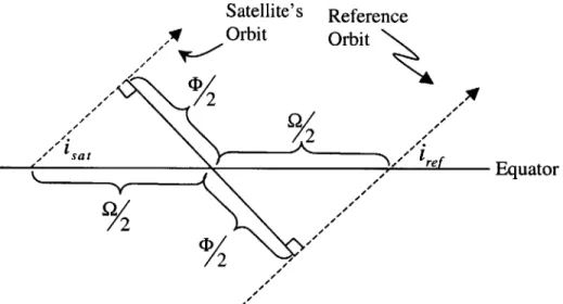
Figure 3-6: Location of the Intersection of the Two Orbital Planes ... 40

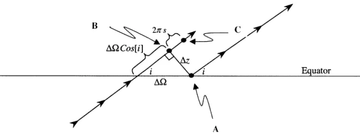
Figure 3-7 : The Moving Intersection of the Orbital Planes ... 41

Figure 3-8: Determining the Amplitude... ₄₄

Figure 3-9: Determining the Amplitude when iref = is ... 45

Figure 4-1 : Variation in the Longitude of the Ascending Node ... 58

Figure 4-2: Origin Motion - Hill's Equations...65

Figure 4-3 : Numerical Solution - Absolute Motion - Solution 1...67

Figure 4-4 : Numerical Solution - Absolute Motion - Solution 2...70

Figure 4-5 : Origin Movement Errors Combined ... 72

Figure 4-6 : Hill's Equations - Relative Motion - Radial Offset ... 74

Figure 4-7 : New Linearized Equations - Relative Motion - Radial Offset...76

Figure 4-8 : New Linearized Equations - Relative Motion - Radial Offset...78

Figure 4-9 : Hill's Equations - Relative Motion - In-Track Offset...79

Figure 4-10 : New Linearized Equations - Relative Motion - In-Track Offset ... 81

Figure 4-11: New Linearized Equations - Relative Motion - In-Track Offset ... 82

Figure 4-12: Hill's Equation - Relative Motion - Cross-Track Offset...84

Figure 4-13: New Linearized Equations - Relative Motion - Cross-track Offset...85

Figure 4-14: Hill's Equations - Relative Motion - Cross-Track Velocity Offset...87

Figure 4-15: Linearized Equations - Relative motion - Cross-Track Velocity Offset...88

Figure 4-16 : Linearized Equations - Relative Motion - Cross Track Velocity Offset.... 90

Figure 5-1 : The Relative Orbit... 95

Chapter 1

INTRODUCTION

Satellite formation flying is the placing of multiple satellites into nearby orbits to form 'clusters' of satellites. These clusters of satellites usually work together to accomplish a mission. There are many benefits to using multiple spacecraft as opposed to one large spacecraft. These include, but are not limited to: increased productivity, reduced mission and launch costs, graceful degradation, on-orbit reconfiguration options, and the ability to accomplish missions that would be unattainable any other way.

One example of a mission that will use formation flying is the Air Force's TechSat 21 mission [1]. The TechSat 21 mission is a distributed satellite system that is a flight demonstration of space-based radar. Interferometry will be used to detect ground-moving targets. The approach of interferometry to obtain high-resolution images is not new. It has been used in many ground-based applications, most notably in the Very Large Array [2]. The VLA is a radio observatory in New Mexico that uses 27 radio dishes, each 82 feet across, to produce an image with the same resolution as a dish 36 km wide. TechSat 21 will employ this same technique of interferometry by using up to 16 satellites in a cluster approximately 500 meters wide. These satellites will work together to produce high-resolution ground target information.

With the desire to place spacecraft into clusters, comes the need to accurately determine and control the position of satellites within the formation. In order to accomplish this, researchers initially turned to Hill's equations, also known as the Clohessy-Willshire equations. Hill's equations are a set of linearized equations that describe the relative motion of two spacecraft in similar near-circular orbits assuming Keplerian central force motion [3]. In the past Hill's equations have been used for rendezvous maneuvers, but these equations have started to find a new use in satellite formation flying.

As will be shown in Chapter 2, much research on satellite formation flying has been accomplished through the use of Hill's equations. These equations are utilized because they are easy to use. They are a set of linearized, constant coefficient differential equations. Because of this, they can be solved analytically and provide a solution that is fairly simple in form and is easy to understand. These solutions allow for an intuitive sense of the relative motion of satellites in clusters. Hill's equations are also used in the design of control laws since the most effective control schemes require a set of constant coefficient, linearized equations. These reasons and more make them the logical first choice in describing relative satellite motion.

However, while Hill's equations have proved very useful, they have several significant limitations. Since they are linear, some error is introduced into the solution. However, linearization errors are not the limiting factor. Hill's equations are derived under the assumption that the disturbance forces acting on the satellites are negligible. This assumption is usually acceptable for most relative motion problems, including rendezvous maneuvers. In rendezvous maneuvers, the spacecraft are usually spaced relatively close, and thus the differential effect on each spacecraft is small. Rendezvous maneuvers are also relatively short in duration, so errors have little time to develop.

For formation flying, the conditions are a little different. Satellites are spaced from meters to kilometers apart. Missions are also on a larger time scale, and errors begin to add up. Because of these two issues, disturbances do have a significant effect on the satellite motion.

The disturbance force cited time and time again as the preventing force from making Hill's equations a completely useful tool is the J2 geopotential disturbance force. Because

the Earth is an oblate spheroid, (it's like a squished basketball bulging out at the equator), the gravitational potential is not constant as the satellite orbits the earth. This disturbance causes many variations over time in the satellite orbital elements. Independent of satellite size or shape, the J2 force is always a dominating presence and cannot be changed.

In the derivation of Hill's equations, the Earth is considered spherical, and the J2

disturbance in not incorporated. Thus, they do not capture the J2 disturbance effects.

Many papers have since been written that quantify the error resulting from their use. Other papers do not use them at all, citing the fact that they do not capture the motion of the satellites correctly.

It appears that there is a need for a set of linearized equations that are as easy and useful as Hill's equations, but at the same time capture the effect of the J2 disturbance force. In

this thesis, a set of linearized, constant coefficient differential equations will be developed that capture the J2 disturbance force.

These new equations are similar to Hill's equations in form. The radial and in-track motion is still coupled, but are separate from the cross-track direction. They are easily solvable, and the solutions look very similar to Hill's equations. However, they capture the J2 disturbance that Hill's equations fail to capture.

Satellite formation designers will now be able to quickly and accurately predict cluster size and shape. They will also be able to design optimal control laws that take into account the effects of the effects of the J2 disturbance force.

Finally, the new linearized equations of motion allow for some new insight into the motion of satellites under the presence of the J2 disturbance force. Cluster 'tumbling' is

discussed as a J2 effect. The cross-track motion has also been analyzed and determined to

be much more complex than previously thought.

The derivation of these equations will be presented in Chapter 3. Following in Chapter 4 is an analysis of the new linearized equations. The solutions to the new linearized equations will be compared against the mean variation in the orbital elements. Then the solutions will be compared to numerical simulation. Concluding in Chapter 5 will be a discussion of the insights gained by using the new linearized equations.

Chapter 2

PREVIOUS WORK

In this section, a brief overview will be given on a selection of papers that deal with the relative positioning, motion, and control of satellites in clusters. Some of the papers presented employ Hill's equations as their sole means of determining the satellite motion. Others cite the errors in Hill's equations, primarily due to differential J2 forces and

calculate the errors incurred by using them. Finally some use non-linear techniques to derive their solutions.

2.1 Using Hill's Equations as the Equations of Motion

There are many different ways of describing satellite motion within a cluster. In the past, when relative motion between satellites has been needed, Hill's equations have been used. This typically was for rendezvous missions where the distance separating the spacecraft was small, and the mission time relatively short. However, due to their ease of use and relatively good accuracy, they make a natural transition to satellite formation flying. Once again the relative motion between two satellites is calculated, but now they are separated by a greater distance and for longer periods of time. The following papers in this section use Hill's equations as the primary means of describing satellite motion.

2.1.1 "Relative Orbit Design Tool"

The first paper discussed is written by Tollefson [4]. He has recently created a software package for satellite formation flying. Using a graphical interface, this software package allows users to rapidly design and test satellite clusters.

In his paper, Tollefson first uses Hill's equations to describe the different types of relative orbits that are possible in a cluster. These relative orbits can be designed in the software

package, and the software is able to output the traditional orbital elements for each satellite in the cluster.

The tool also has many graphical interfaces and displays that allow the user to see the cluster in many different views. This allows a user to change the parameters of the cluster while noting the effect it has on the cluster. Finally, the tool has three additional features: a two-body orbit propagator (for elliptical reference orbits), collision detection, and the ability to output the orbital elements of the cluster into Satellite Tool Kit. Overall, the paper describes a tool that allows for the quick and easy design of satellite clusters.

2.1.2 "TechSat 21 Cluster Design Using AI Approaches and the

Cornwell Metric"

The next paper is by Kong, Tollefson, Skinner, and Rosenstock [5]. In their paper, they describe an approach for choosing an optimal cluster design. Their research is primarily focused on the TechSat 21 mission.

Because of the many different configurations possible for a satellite cluster, intelligent search algorithms are utilized to choose an optimal design. Two different metrics are disused for possible use in the optimization routine: Point Spread Functions, and the Cornwell Metric. Using Hill's equations as the satellites' equations of motion, the paper shows that intelligent search algorithms are nearly as effective as evaluating the whole trade space. However, intelligent algorithms are faster by three orders of magnitude. The paper also demonstrates that there are potentially new cluster designs for the TechSat 21 mission that may be better than current designs.

2.1.3 "Geometry and Control of Satellite Formations"

A paper by Yeh and Sparks [6] utilizes Hill's equations to present some interesting

geometrical relationships for satellites in clusters. For example, Hill's equations predict that 'orbits' of one satellite around another satellite are restricted to the intersection of a plane and an elliptical cylinder with an eccentricity of r3-/2. This allows for some

interesting insight into which 'orbits' are possible, and which ones cannot be designed. This same technique is used to help describe satellite 'tumbling' in section 5.3.

The paper also presents a control law using Hill's equations. Disturbances and control forces are placed onto the right hand side of Hill's equations as forcing functions. These control laws allow for the cluster initialization and adjustment. The author states, that Hill's equations are a starting point for designing control laws, but also states that these control laws may be inefficient when disturbances such as the J2 disturbance force are

incorporated.

2.1.4 "Satellite Formation Flying Design and Evolution"

The paper by Sabol, Burns, and McLaughlin, [7] gives a brief overview on the evolution of cluster design, and utilizes Hill's equations to describe the different types of cluster designs. Each cluster design is placed into a simulator with realistic dynamics, and the results from each simulation are presented and discussed. The effects of the J2

disturbance force are noted and a control scheme is presented for formation keeping. Using Gauss' variation of parameters, the minimum Av needed to counteract the J2

disturbance force was calculated. This required Av provides a minimum Av needed for station keeping in the presence of the J2 disturbance force.

2.1.5 "Linear Control of Satellite Formation Flying"

In this paper by Sparks [8], Hill's equations are once again used to define the motion of satellites in the cluster. The J2 disturbance force was labeled as the most destabilizing

perturbation. Just like in the previous paper, Gauss' variation of parameters was used to derive a minimum value for the total Av needed to counteract the effects of the J2

disturbance.

A discrete time linear control law was then developed. This control law was placed into

a simulator and was able to produce approximately the same Av as the theoretical minimum given by Gauss' variation of parameters.

18 Chapter 2 - Previous Work

2.2

Quantifying the Errors of Utilizing Hill's Equations

While the previous papers have used Hill's equations as a means of describing satellite motion, other papers analyze the errors that are incurred by using them.

2.2.1 "Gravitational Perturbations, Nonlinearity and Circular Orbit

Assumption Effects on Formation Flying Control Strategies"

The J2 disturbance force affects each satellite in a cluster differently. These differential

forces cause the cluster to change shape and separate. An analytical method by Alfriend, Schaub, and Gim [9] is used to evaluate the differential forces, and the effects of using Hill's equations.

In the paper, a state transition matrix is calculated that relates the changes in the orbital elements to changes in the local coordinate frame. The resulting equations are compared

to Hill's equations in the presence of J2 perturbations, and eccentric reference orbits. The

results showed that using this state transition matrix provided better results than that obtained with Hill's equations.

2.3 Eccentric Orbits

Due to the assumptions made in the derivation of Hill's equations, satellite clusters have traditionally been considered to be in near-circular obits. However, there are some benefits to placing satellite clusters into eccentric orbits. This allows for longer dwell time over regions of interest, and shorter occultation time. Since Hill's equations are based on a circular reference orbit, they fail for eccentric reference orbits.

First introduced by Lauden [10], time varying linear equations of motion can be developed utilizing an elliptical reference orbit. The resulting differential equations, while no longer time-invariant can be solved analytically.

Chapter 2 - Previous Work 19

2.3.1 "Relative Dynamics & Control of Spacecraft Formations in

eccentric Orbits"

Inalhan and Hall [11] have expanded the topic of eccentric reference orbits to incorporate satellite clusters. In their paper, they derive the linearized time varying equations of motion, and present the homogenous solutions. They also present initial conditions that produce periodic solutions, thus preventing satellites from drifting apart due to different orbital periods. The solutions to the elliptical linearized equations are then compared to Hill's equations for modeling satellite clusters in elliptical orbits. The errors incurred by utilizing Hill's equations are presented.

2.4 Non-Linear Techniques

2.4.1 "J

The J2 disturbance causes many changes to a satellite's orbital elements over time. This

includes precession of the ascending node, argument of periapsis, and changes to the mean motion. In a satellite cluster, the differential changes in the orbital elements causes satellites clusters to change form and drift apart.

In this paper by Schaub and Alfriend [12], an analytical technique is used to derive a class of orbits that are termed 'J2 invariant' orbits. Satellites placed into 'J2 invariant'

orbits are not immune to the J2 disturbance force, but instead two satellites placed into

these orbits will have the same drift, and thus the cluster remains together. The 'J2

invariant' orbits are created by using two first order conditions that determine the correct differences in semi-major axis, eccentricity, and inclination.

2.4.2 "Impulsive Spacecraft Formation Flying Control to Establish

Specific Mean Orbital Elements"

In this paper by Schaub and Alfriend [13], an impulsive control algorithm is developed using mean orbital elements. The change from osculating orbital elements to mean orbital elements seems to have a two-fold purpose. The first is that small periodic

variations are not captured by the control system and thus propellant is not wasted counteracting these variations. Instead only the secular drift in any of the orbital elements is corrected for.

The second reason for switching to mean orbital elements is because impulsive maneuvers are only applied once or twice during an orbital period. If the amount of thrust applied is dependent on the current orbital elements, the average orbital elements need to be used otherwise periodic variations may cause errors.

The reason why impulsive maneuvers are only performed once or twice an orbit, is because the paper once again uses Gauss' variation of parameters. This allows the controller to choose almost independently which orbital element to change and when to apply that thrust at the most opportune time. The opportune time to thrust usually only happens once or twice an orbit.

Numerical simulations were conducted to verify that the controller was capable of controlling the variation in the mean orbital elements in the presence of disturbances, and cluster misalignments.

2.5

_{Linearized Equations of Motion that Incorporate the J}

Disturbance Force

2.5.1 "Mitigation of Differential Perturbations in Clusters of Formation

Flying Satellites"

This paper by Sedwick, Miller and Kong [14] analyzed an assortment of perturbation effects of a satellite cluster. These included a non-spherical Earth, atmospheric drag, solar radiation pressure, and magnetic field interactions. This was first done by using a non-dimensional approach to determine the scaling of each perturbation effect.

The next section of the paper looks at each perturbation effect in more detail. Focusing on the TechSat 21 mission, only polar orbits were analyzed, and only in-plane disturbances were accounted for. For the J2disturbance analysis, the J2disturbance force

Chaoter 2 - Previous Work 20

is added to the right side of Hill's equations as a disturbance force. In order to calculate the differential J2 effects, a nominal trajectory is projected into the J2 force to produce a new forcing function. The resonant terms in this forcing function are responsible for the secular drift in the relative motion, and the Av needed to counteract these forces is presented.

The other disturbance forces, including the error due to the linearization, are also looked at in more detail. The resulting total Av necessary for station keeping is analyzed and presented for the TechSat 21 mission.

2.5.2

"A Perturbative Analysis of Geopotential Disturbances for

Satellite Formation Flying"

Written by this author, the paper [15] is written on the same subject as this thesis. In this paper, both the gradient of the J2 force and the gradient of the spherical gravitational

potential are incorporated to from a new set of linearized equations. This is the same derivation that is presented in the next chapter. At the time of the writing, the cross-track motion was just being understood, and was not fully explained. This thesis will complete the analysis of the cross-track motion and provides the final linearized equations of motion.

2.6 Conclusion

There has been a recent flurry of research on satellite formation flying. This research falls into three general categories: papers that utilize Hill's equations, papers that show Hill's equations do not capture the J2 disturbance effects, and papers that use a non-linear method of capturing the J₂ disturbance effects.

From this survey of current research, there appears to be a need for a set of linearized equations that are easy to use, but at the same time are able to capture the J2 disturbance. In the next chapter a set of linearized equations of motion will be presented that captures the J2 disturbance force but at the same time is as easy to use as Hill's equations.

Chapter 3

DERIVATION OF THE NEW

LINEARIZED EQUATIONS OF

MOTION

In this chapter, a new set of linearized equations of motion will be developed. These equations will be like Hill's equations in form, but will also capture the effects of the J2

disturbance force.

3.1 Approach Overview

The first step in the derivation is to write the equation of motion of a satellite under the influence of the J2 disturbance in its simplest form, where g(i) is the gravitational force

due to a spherical Earth, and 2(V)is the J2 disturbance force.

r = g(i)+J2(V) (3.1)

While this equation completely describes the motion of a satellite under the influence of the J2 disturbance, it is not necessarily useful. First it cannot be solved analytically.

Second, it is not useful in visualizing the relative motion that is present in satellite clusters.

The solution to these problems is to introduce a reference orbit. This reference orbit can be tailored to be any type of orbit. In this thesis, four different reference orbits will be used: an unperturbed circular orbit (Hill's Equations), a circular orbit with a modified period (Solution 1), a circular orbit with modified period, inclination, and longitude of the ascending node (Solution 2), and finally the center of the cluster itself (Relative Motion).

The next step in the derivation is to linearize both the standard gravitational term and the J2disturbance around this reference orbit.

w

= i ,- )+e2(=

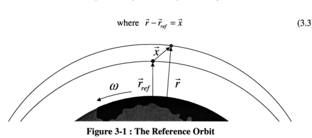
)-where ?-, =X

(3.2)

(3.3)

Figure 3-1 : The Reference Orbit

Since we are interested in only the relative motion between the satellite and the reference orbit, we subtract off the motion of the reference orbit from the equation of motion of the satellite.

r -ef = (ef) + Vk( 'ef +j ₂( 'ref+ Vj2( 'ref) xrref (3.4)

Which can be simplified to

=

g(ef )+V (,ef)

In the rotating coordinate system of the reference orbit, the initial equation of motion is

x + 2x k +& xC +Cx(o x )= g('ef) + Vg(, ').e + j 2(,ef +Vj 2(i,ef)- - ,ef (3.6)

It will be shown later that Vj 2(ie) is not constant, and since we are looking for constant

coefficients, the time average of the gradient is taken. The resulting equation is

+2 + =

(3.7)

g(,ef ) + g(',ef )-+ j 2(ef ) + fVJ 2(ief)dO - -i

2r0 -re

Equation (3.7) forms the basic equation that will be used throughout this paper. The main variations to it will be in the choice of the reference orbit, and corrections to the cross-track motion. These topics and a more detailed analysis are discussed in section

3.3-3.6

3.2 The Coordinate System

Before going through a detailed analysis, the four coordinate systems used throughout this thesis will be described. One system is an inertial coordinate system used to represent the absolute position of the reference orbit while the other three coordinate systems are body fixed coordinate systems.

3.2.1 The1

- Z

Inertial Coordinate System

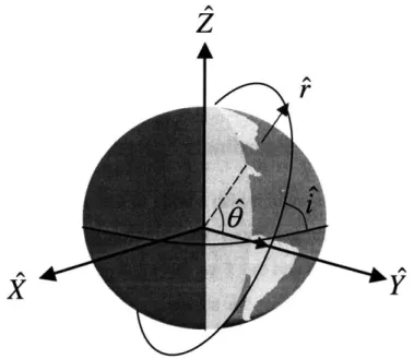
The X - Y - Z inertial coordinate system is an Earth centered system. The X - Y plane

coincides with the equatorial plane, and the Z vector points through the North Pole. See Figure 3-2.

2

r

u T

Figure 3-2: The X -Y -Z and r^ -0 -i Coordinate Systems

3.2.2 The r

-

i

Body Fixed Coordinate System

The second coordinate system used is a spherical coordinate system. The r points in the radial direction, i is the azimuthal angle measured around the line of nodes, and $ is the co-latitude measured from the ascending node which acts as the "pole" of the spherical system. See Figure 3-2.

3.2.3 The

N Body Fixed Coordinate System

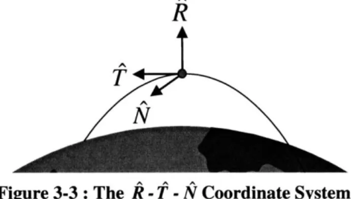
The third coordinate system is a body fixed coordinate system with the origin located at the reference satellite. The R vector (radial) points in the radial direction. The N vector (normal) is perpendicular to the orbital plane and points in the direction of the angular momentum vector. Finally the T vector (tangential) completes the orthogonal triad, and points in the direction of movement. See Figure 3-3.

R

N

Figure 3-3: The R -T -N Coordinate System

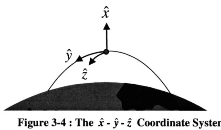
3.2.4 The X - - Body Fixed Coordinate System

The fourth and final coordinate system is also a body fixed coordinate system that is very much like the R - T - N coordinate system. The X vector points in the R direction, the

j

j

j

M-1 t 76

Chapter 3 - Derivation 27

X

Figure 3-4: The .^ -y -z Coordinate System

3.2.5

Converting Between the Body Fixed Coordinate Systems

Conversion between the body fixed coordinate systems is fairly straightforward. The radial vector in each coordinate system completely coincides. The T vector,

j

$

defined as a curvilinear system but as rectangular.

However, the only use of the R - T - N is when the J2 disturbance force is presented.

This does not pose a problem because only a direction is calculated using this coordinate system and not a position. Therefore one can freely switch between the R - T - N system

and any of the other body fixed coordinate systems described here when describing a direction or a force.

3.3 Detailed Derivation

-

Absolute Motion

-

Solution 1

Section 3.3 will present the initial derivation of the new linearized equations of motion. The steps followed here will be the same as outlined in section 3.1. Each step will be shown in more detail, and a reference orbit will be chosen. The result will be a set of linearized, constant coefficient differential equations. The analytic solution to these equations will also be presented.

28 Chapter 3 - Derivation

3.3.1 The Basic Equations of Motion

The first step is to start off with the analytical equation of motion

r =q) g(+ 2(T) (3.8)

where g(T) is the gravitational force due to a spherical Earth,

( - (3.9)

r

andJ2(') is the force due to the J2 disturbance [3].

i2(i)= 3 J2 PRe [( 3 3Sin2i Sin2O)R

2 r (3.10)

+(2 Sin2_{i Sin0 Cos0)T+(2 Sin i Cos i Sin 0) N]}

where Reis the radius of the Earth.

3.3.2 The Unperturbed Circular Reference Orbit

The next step is to introduce the reference orbit. For simplicity, a circular reference orbit only under the gravitational influence of a spherical Earth is initially used. This is the same reference orbit used in Hill's equations. The position of the reference orbit is denoted as .ef

efg(ref) (3.11)

3.3.3 Linearization of the Gravitational Terms

The next step in the derivation is to linearize the gravitational terms with respect to the reference orbit. The resulting equation of motion is

Using a spherical coordinate system (r -I) the gradient of the k(F) gravitational force is calculated. The result is a 2nd order tensor.

2-L 0 0 0 0 0 -(3.13)

The J2 disturbance force (equation (3.10)) is given in R - T - N^ coordinates. However

the equation can be transferred directly to a r^ - - t coordinate system without any loss of generality. The resulting gradient is

VJ2(r,0,i)= (1-- 3Sin2i Sin2₀₎ Sin 2_{i Sin 20} Sin 2i Sin G Sin2_{i Sin 20} 1 2 17 2 -- Sin i (

_

3.3.4 Relative Motion

As in the derivation of Hill's equations, motion is taken with respect to the reference

orbit. This relative motion is denoted as i. See Figure 3-1

i =T -ref (3.15)

Since the reference orbit is rotating, rotational terms are needed when calculating the relative motion of the satellites. Note the 'rel' subscripts will be dropped in the remainder of the text.

Xre =r -261 x ,,, -c>x x -co x (Co x i)(

6pJ_2R2 ref

(3.14) 29

30 Chapter 3 - Derivation

Co is the rotational rate of the body fixed coordinate system, and thus the angular velocity

of the coordinate system. For a circular reference orbit

= 2 = n z (3.17)

Substituting equation (3.12) into equation (3.16) and re-arranging the terms yields

C

+2xi +>x+sx(eCx3) = g(,ef)+ V( if )i + j 2(ef )+VJ2 (2,f ) - ,f(

3 ₁8₎

3.3.5

Time Averaging the J

Equation (3.18) is a linearized equation of motion, however, the problem arises that

VJ2(,ef) is not constant except for equatorial orbits. An approximate solution to this

problem is to take the time average of the VJ2() term.

4s 0

0

2 r d r [0 0 -3sj _(3.19)

where s = 8 (1+3 Cos 2i)

8r2

Equation (3.18) now becomes

x+2s x i+ (>x + x (@x i)

1 2"r (3.20)

= ('ref )+ vg(Fef). + j 2 (Tef ) +

r

0

3.3.6 Adjusting the Period of the Reference Orbit

Under the influence of the J2 disturbance force, the perturbed satellite will have a different orbital period than when unperturbed. Because of this discrepancy, the satellites

-h ntr - - -.-- tio 3

down. To fix this problem, the period of the reference orbit must be adjusted to match the period of the satellites in the cluster.

The change in period due to the J2 disturbance can be found from the average J2 force

(not to be confused with the time average of the gradient of the J2 term taken above). The

equation of motion of the reference orbit, see equation (3.11), now becomes

1 2;r ',ef =( ef )+- fJ 2(ief )d0 (3.21) 2r0 where 1 -- J2(i) do = -nr s x (3.22) S = 82 * (1+ 3 Cos 2i) 8r2

Now that the reference orbit has a new period, the angular velocity vector of the rotating coordinate system must also be updated.

r2;rxei,)$ + Z(gd (3.23)

ref 2; 0

which gives

n=nc2

(3.24)

3.3.7 Final Solution - Circular Reference Orbit - Solution 1

Equation (3.20) becomes

x + 26 x i + 6 x -+ 6 x (6 x i)=

1 2 2; (3.25)

Vk(',f)-'+Z2(7,f)+-f VZ2(Q, )d6 -i- f2(re )d0

Substituting in all of the terms the resulting equations of motion are (in k -

j

coordinates)

-2 (n c) j -(5c2 -2)n2x = -3n2 2 (I 1 3 Sin2i Sin2(n c t) (1+3 Cos 2i))

r 2 2 8

2(nc)i -n j - Sin 2i Sin (net)0 Cos (n ct) rref

O+(C2 - 2) nJZ=-n 2 -E-Sin i Cos i Sin (n ct)

ref

(3.26)

Because these equations are linear, constant coefficient differential equations, they can be easily solved. The results are presented below. The initial conditions, o &

j5,

x = (x0 - a) Cos(n

t4Vs)

t1

t.

IV

-y =- (x0 - a) Sin(ntv s + yo Cos(nt

I)-

VI7

z = zo Cos(n t1+ 3s) + z Sin(n t1+ 3s)+ n-1+ 3s

#3(1I+

(3.27) 3n J2

j;o=-2ncx

)

Chaner - Deivaion33

3.4 Detailed Derivation Cont.

-

Absolute Motion

-

Solution 2

While the above equations of motion are a vast improvement over Hill's equations when incorporating the J2 disturbance force, more can be done. Even though the orbital period

of the reference orbit has been adjusted to match the perturbed satellite they still drift apart due to separation of the longitude of the ascending node. This section will derive an expression for a new reference orbit that has the same drift in the longitude of the ascending node as the perturbed satellite. This will be accomplished by using mean variations in the orbital elements. It should be noted that this expression is only an approximate solution to the new reference orbit and modeling errors are introduced.

3.4.1 Re-adjusting the Reference Orbit

While the current reference orbit and the satellites in the cluster have the same orbital period, they still drift apart. This is due to the fact that the longitude of the ascending node of a satellite will drift under the influence of the J2 disturbance.

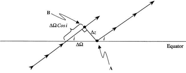
B

AA Cos i

AO Equator

A

Figure 3-5: The Effects of a Changing Argument of Periapsis

If both the reference orbit and a satellite in the cluster start at point A, after one orbital

period the perturbed satellite will be at point B while the current reference orbit will return to point A. The satellites are now separated by a distance Az. After two orbital

periods, the satellites will be separated by an additional Az, and this process will continue causing the satellites to drift farther and farther apart. See Figure 3-5.

Because the J2 disturbance force is causing this separation, the solution to this problem is

to determine the aspect of the J2 disturbance that causes the drift in the 2 direction and

incorporate it into the reference orbit.

Using Gauss' mean variation in the orbital elements [3], the normal component of the J2

force is responsible for the drift in the longitude of the ascending node. Applying the normal component of the J2 disturbance force to the reference orbit results in

,ef g(ref )+ 2j (ief)d6+j2 2(i)ef-N (3.28) 0

With the addition of this force onto the reference orbit, both the satellite and the reference orbit will have a drift in the longitude of the ascending node. Thus, the satellites will not drift apart. It should be noted that differential J2 effects due to the perturbed satellite and

the reference orbit having different inclinations may still cause differential drift in the two orbits, but this drift is on a much smaller scale and will be accounted for in section

3.5

3.4.2 Describing the New Reference Orbit

With the addition of the new forcing term onto the reference orbit, it is not easy to analytically describe the motion of the new reference orbit. One solution is to look at the mean variation of the orbital elements.

The position of the reference satellite in X - Y - Z Earth-centered inertial coordinates is [3]

ie = re (Cos 2 Cos 6 - Sin Q Sin G Cos i)x

+ r,,f (Sin Q Cos + Cos Q Sin 0 Cos i)Y (3.29)

+ r,.f (Sin 0 Sin i)Z

Chaner - Deivaion35

The normal component of the J2 disturbance has an effect on four out of the six orbital

elements:

ai

C

3JJ

R

r7/ 21~ RE Cos iSin 2 0 3JLJ_-2R 2. Cos i Sin2_O r 72 (3.30) at a OtKNormal)Normal Force Force

The above differential equations of motion of the orbital elements are not easily solved, but a good approximation can be made by assuming a constant inclination.

3 1-uJ R 2

i(t) = io - j 2 'e Cos i Sini Sin2 (k t)

2kr7/2

3v/J_{t= -2'} 2R2 _{Cos i (tk}.

2k r

O(t)=nct+ "2Re Cos 2_i(t 2kr7 /2 Sin(2kt) 2 Sin(2k t) 2 3 ,J2R2 ₂ k =nc+ 3 /*2 Cos2i 2 r''2

Equation (3.31) can now be substituted back into equation (3.29) to provide an approximate equation of motion for the reference orbit.

(3.31)

3.4.3 Angular Rotation Rate of the New Reference Orbit

Now that we have modified the reference orbit, the angular velocity

C

(dQ . di

w -Q=( SiniSin 0+ - i Cos O)

dt) dt

(dC' di'

+( Sin i Cos 0 - i) Sin 0)9

dt dt Y(3.32)

+( - ) + _I Cosi)2

dt dt

Substituting in equation (3.31) and taking the time average results in

C = c n 2 (3.33)

This is the same angular rate as derived with the previous reference orbit used in the 1st

solution. This makes sense because a normal force should not affect the angular rotational rate.

3.4.4 Final Solution - New Reference Orbit - Solution 2

Because we have added a component of the J2 disturbance to the reference orbit, that

component must be subtracted from the equations of motion. The resulting equations of motion are

x +2@xx + Ox -+Cox(ox i)=

1 21r 2z (3.34)

V (,f )-i+ j 2 ( ,f )+-f VZ2( ,r )d -.i -- 2 2( ,)d -Z2 ( , )-N

ChaDter 3 - Derivation 7

Substituting the appropriate terms into the equations results in

-2

(n

9+2(nc)k=

-3n2j2R 2 (1 3 Sin2i Sin

2_{(k t)}

rre 2 2

-3n 2j 2 _Sin2i Sin(kt) Cos(kt)

rref (1+3 Cos2iref) 8 (3.35) S+(3c 2 _{- 2)n2} z = 0

These can be solved, resulting in

x = (xO -a

2) Cos(nt-1i §)+ y0 Sin(nt vi )+a 2 Cos(2k t)

2

NIT+-y =-2 (xO -a 2) Sin(nt i7 s) + yo Cos(nt' si7)+Q 2 Sin(2kt)

z = zo Cos(n t1I+3s)+ ZO Sin(n141+3s) n .1+3 s

po=-2n

k =fnI+ s + 3nJ2Re Cos2

2r2ref2 g

(3.36)

3.5

Correcting Out of Plane Motion

-

Solution 3

This next section will address a problem with the linearized equations of motion as derived in the previous section. More specifically, the cross-track motion is not currently modeled correctly. The cross-track motion is deceivingly the most complex motion seen

by the satellite cluster. While the linearized differential equations of motion look simple

for the

Q

3.5.1 Why do the linearized equations of motion fail?

Under the influence of the J2 disturbance force, the orbital planes rotate around the Z axis (the north pole). This is due to the fact that the J2 disturbance force is symmetric across the equator. The new linearized equations of motion, instead of predicting that the orbital planes rotate around the Z axis, predict that the orbital planes rotate around the vector normal to the reference orbit. So in the equatorial case, the linearized equations of motion correctly represent the out of plane motion, (the normal vector to the orbital plane points in the same direction as Z ). However, for inclinations other than equatorial, the linearized equations of motion incorrectly model the out of plane motion.

And again the question is why do the linearized equations of motion fail? The reason is that the J2 disturbance force is modeled by taking the time average of the gradient of the

J2 disturbance force (see section 3.3.5). This assumption causes the J2 disturbance to

appear symmetrical about the current reference orbital plane. Once again, for an equatorial orbit, the time average of the J2 disturbance is not a simplification since the J2 disturbance force is always a constant, and symmetrical about the equator.

For in-plane motion, the assumption of the time averaged J2 disturbance is not a

significant error and no changes are required. However for cross-track motion, the error is significant. In this section we will develop a new equation for the out of plane motion based on the geometry of the moving orbital planes. At the same time, the analysis will

be expanded so that differential J2 effects due to different satellite inclinations will be

taken into account.

3.5.2 Description of Cross-Track Motion

Cross-track motion is due solely to the fact that the satellite orbit and the associated reference orbit are not coplanar. It is a periodic motion that is equal to zero when the two orbital planes intersect, and is at a maximum 900 away from the intersection of the planes. The intersection of the two planes is based on differences in the inclination and longitude of the ascending node between the orbital planes. Under the influence of the J2 disturbance force, these orbital planes move.

As these orbital planes move, both the period and the amplitude of the periodic terms change. This changing is not linear, and spherical trigonometry will be used to derive the out-of-plane motion. Once the period B(t) and amplitude A(t) are known as functions of time, the equation for out of plane motion can be written in the form

r

z = A(t) Z0 Cos(B(t) t)+ n +sSin(B(t) t) (3.37)

A(O) A(0)

3.5.3 The Period of the Periodic Terms

The period of the periodic terms is defined as the length of time between crossing the intersection of the two planes and returning to that same intersection. When the orbital planes move, the location of this intersection also changes, and thus the period of the periodic terms is also changing. In this section, the distance between the intersections of the orbital planes from one pass to the next will be calculated. Since the velocity of the satellite is known, the resulting period can be determined.

40 Chanter 3 - Derivation

Satellite's Orbit

Orbit

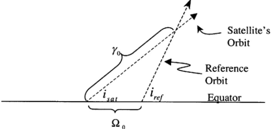
Figure 3-6: Location of the Intersection of the Two Orbital Planes

Figure 3-6 shows the orbit of a reference orbit, and the orbit of the satellite as they cross the equator. iref and i,, are the inclination of the reference orbit and the satellite

respectively. Q0 is the initial angular separation of the longitude of the ascending node between the two orbits. yo is the angular distance from the satellite's equatorial crossing,

and the crossing of the two orbits. yo can be calculated using spherical trigonometry.

Yo = C Cos' i Cos 0 -Cotiref Sin is,(3

yo = Cot ( i 0(3.38)

Sin2,

)o

Because of the J2 disturbance force, the orbits' longitude of the ascending node will

precess. This precession of the two orbital planes causes the location of the crossing of the two orbital planes to change. The extra distance that the satellite must travel before crossing the reference orbit can be calculated using Figure 3-7.

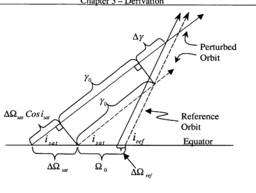
Chanter 'I - Derivntion 41 AY AQsat COsa,

ftf

Figure 3-7: The Moving Intersection of the Orbital Planes

Figure 3-7 shows the changing location of the orbital plane crossing. The dashed line represents the initial orbital plane, while the solid line is the orbital plane at a later time. The location of the orbital plane crossing can be described by a change in the distance between the satellites equatorial crossing and the crossing of the reference orbit Ay.

CosiCosCnet -Coti Sini

Sin ,net (3.39)

ant 0 Msat -Aref

3 J2 Re t (3.40)

sat 2 COS isat

2 _r

3 J2 nR2 t

ref ~ _ 2 ref

2 re

Equation (3.39) determines the extra distance that the satellite must travel (Ay) as a function of time. While this solution provides an accurate means of determining this

A2sat

41

distance, it is a little tedious to calculate. A first order approximation can be made by calculating the derivative of y with respect to Q.

dy = _{Sin i,ff (Cos i,f Sin isa, Cos Qo -Cos i, Sin i, )}

dK (Cos iref Sinisa, -Cos isa, Sin irf Cos 20)2 _{+ (Sin irefSin 2}

0)2

From this equation, Ay can be calculated as

Ay -Y Anet - AQsat COS sat (3.42)

d92

Which is a linear function in time, and can be written as

Ay=bt (3.43)

where b is a constant.

Both methods provide roughly the same solution. While equation (3.39) is more exact, equation (3.42) is easier to implement once the derivative has been calculated.

Equation (3.42) also allows for some insight into the motion of the location of the orbital plane crossing. When the difference between iref and ,satis small, and A2 is small,

dy/dQ becomes very large. Thus small changes in A2,net can result in large changes in Ay. This is due to the relative orientation of the orbital planes and the axis about which they rotate.

This motion can be thought of as a scissoring effect. When a pair of scissors is opened, the point of intersection of the two blades moves very rapidly from the tips back. As the handle is opened further, the rate at which the intersection of the two blades moves towards the handles slows down. With orbital planes, the location of the intersection of the orbital planes will move very quickly away from the equator, and then as it approaches the poles it will slow down.

Once a function for Ay has been calculated, the arguments of the periodic terms can be calculated.

A y

B(t)= nc

-t (3.44)

If the first order approximation of Ay, equation (3.41) and (3.42), is

calculate A y then B(t) is a constant.

B(t)= nc - b (3.45)

Also, if the orbital planes have no differential movement and the same inclination,

A,net =0 and iref = i ,, 1 then

B(t) = n c - b = k k =nc+ 2 Cos2i 2rref (3.46) used to Chapter 3 - Derivation ₄₃

3.5.4

Amplitude

The amplitude of the out-of-plane terms is dependent on the maximum separation between the two different orbital planes. This can once again be calculated with

spherical trigonometry.

Satellite's Orbit

Orbit

(DI N,

Figure 3-8: Determining the Amplitude

From Figure 3-8, it can be seen that the maximum amplitude is based only on the

inclination of both orbits, and their separation at the equator.

The angle (D can be calculated using

900

Q1)(t) = COS-' (Cos isat Cos iref + Sin isat Sin irf Cos Q(t)) (3.47)

where 92 is the time varying separation of the longitude of the ascending nodes.

Now that D has been determined as a function of time, the amplitude of the out of plane motion can be defined as

A(t)= ref (t)= ref Cos-'(Cosisat Cosirf + Sins, Siniref Cos4(t))

44 Chapter 3 - Derivation

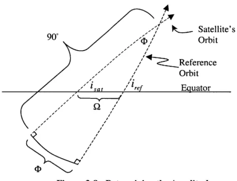
There are times when the inclination of the reference orbit and the inclination of the satellite are identical. When this is the case, the two orbital planes intersect at 6 = 900,

and using Figure 3-9 the amplitude can be more simply calculated by

CD(t)= 2Sin-'(Sin i Sin

)

2

When 92 is small, this can be approximated by

CD(t) ~ Q(t) Sin i (3.50) Satellite's _Reference Orbit _Orbit 7./2 S'/"2 -, sat _1re Equator 2

Figure 3-9: Determining the Amplitude when ref = isa

3.5.5

Final Out-of-Plane Motion

We can now write the out-of-plane motion as

z = A(t) zo Cos(B(t) t) + Sin(B(t) t)

A(O) A(O)

A(t) = refD(t) (3.51)

B(t)= nc -AY

t

When differential motion is not taken into account, there is no change in the amplitude of the cross track terms ( A(t) is a constant). B(t) is also a constant. The equations of motion greatly simplify producing

z = zo Cos(k t)+ zo Sin(k t) (3.52)

n-1+3s

3.6 Relative Motion

While the motion of a satellite with respect to the reference orbit is interesting, what really matters in formation flying is the relative motion of one satellite with respect to another satellite in the cluster.

The equations of motion that describe differential motion can be obtained in two different ways. First, the motion of each satellite can be calculated using the above equations of absolute motion for each satellite. Then this motion is subtracted from one another to produce the relative motion. Otherwise, the equations of motion can be derived by creating a set of differential equations again. Both methods will produce the same results, but the latter is shown here.

Deriving the relative motion can be accomplished by applying the substitution of

x2 -1 =

(53

46

Chanter 3 - Deriv-tin 7

into equation (3.34). i2 and 2, are the relative positions of two satellites in the cluster.

A + 26x A + xi +Cox (CoxA) =V (f + Vj 2('ef)d6- A (3.54)

3.6.1 Final Relative Motion Equations

-

No Cross-Track Corrections

Substituting in the appropriate terms results in the following differential equations of motion in ^ -

j

i- 2(n c) (5c2 _-2)n2x =0

9+2(n

&+(3c2 -2) n2_{z =0}

It should be noted that this is just the homogenous solution to the equations derived in the

1

0 and 2 nd solutions above.

Solving the differential equations results in

x = xoCos(VIs nt) + 2JiT)'yo Sin(i~

7

y 2A- xs Sin(17 n t) + yoCos(V1 7s n t)

z = zoCos(n- + 3s t)+ co _ n yo (1- s) 2 .,/ -+ where s = 2 (1+ 3 Cos 2i,,, 8r.f (3.56)

fo