Development and experimental verification of damping enhancement methodologies for space structures

DEVELOPMENT AND EXPERIMENTAL VERIFICATION OF DAMPING ENHANCEMENT METHODOLOGIES FOR SPACE STRUCTURES

by

NESBITT WARD HAGOOD IV B.S., Massachusetts Institute of Technology

(1985)

SUBMITTED IN PARTIAL FULFILLMENT OF THE REQUIREMENTS FOR THE DEGREE OF

MASTER OF SCIENCE

IN AERONAUTICS AND ASTRONAUTICS

at the

MASSACHUSETTS INSTITUTE OF TECHNOLOGY

September 1988

© Massachusetts Institute of Technology, 1988

Signature of Author

Certified by

Accepted by

Department of Aeronautics and Astronautics

August 12, 1988 7

Profesr dward F. Crawley Thesis Supervisor

(.

tI

o fso

IQach

man

Chairman, Departmental Graduate Committee

MASSHUSEIS ISTmIE .' r

OF TECHNOLOGY . .

SEP 07 1988 -" 'e '

· _r

DEVELOPMENT AND EXPERIMENTAL VERIFICATION OF DAMPING ENHANCEMENT METHODOLOGIES FOR SPACE STRUCTURES

by

NESBITT WARD HAGOOD IV

Submitted to the Department of Aeronautics and Astronautics on

August 12, 1988

in partial fulfillment of the requirements for the Degree of Master of Science in Aeronautics and Astronautics

ABSTRACT

A frequency domain system modelling technique is developed for

mechanical systems. The technique is derived from Tellegen's Theorem for electrical networks and is applied to discrete mechanical systems. The elements are modelled in terms of their mechanical impedances. A global system model is assembled from the constitutive impedances. The global system model is used to determine the model exact pole locations and system energy dissipation and storage properties. An approximate method for finding modal frequencies and loss factors using the system impedance matrix and assumed modeshapes is developed. This method reduces to

Rayleigh's Quotient in the case of an undamped system.

Impedance models for several damping enhancement mechanisms are presented. Among these are models for viscoelastic materials, the classical proof mass damper, and a new damping enhancement concept called the

shunted piezoelectric. The shunted piezoelectric damping mechanism is

based on a piezoelectric material which has its electroded surfaces shunted by

an arbitrary electrical circuit. Methods are developed for analyzing this

special damper and optimizing its damping properties in the case of shunting by a resister or by a resonant circuit. Parallels are drawn between the resistive

shunted piezoelectric and viscoelastic materials and between the resonant

shunted piezoelectric and the classical proof mass damper.

Experiments were conducted on a 5 meter, 10 bay box truss with a quasi

free-free 3 dimensional suspension. A tunable, linear electromechanical driver

was implemented for use as a proof mass damper. Electrical feedback of the

proof mass position and velocity enabled accurate tuning of the dampers resonant frequency and internal damping. Piezoelectric truss members were designed and constructed for implementation of the shunted piezoelectric

truss members. In the resonant shunted piezoelectric experiments the tuning of the piezoelectrics was accomplished by creation of an "active" variable

inductor.

Experiments were conducted to test truss structure dynamics and the

damping enhancement concepts. These tests were compared to the analytical

results obtained from the-frequency domain system modelling technique. The proof mass damper implementation was found to increase system

damping from 0.6% of critical to 6.4% of critical with a system mass increase of 2.7%. The resonant shunted piezoelectric increase system damping to 6.0%

with a similar mass penalty. These resonant dampers were found to have negligible effect on the system modes other than the mode to which they

were tuned. The analytical model was found to be capable of predicting the

global system damping with these two concepts.

Thesis Supervisor: Dr. Edward Crawley

Acknowledgements

I would like to thank my advisor, Professor Edward Crawley, for giving

me the opportunity to conduct this research and for his guidance and time

along the way. I would also like to thank Professor Andreas von Flotow for

his support, advice, and humor when nothing seemed to work.

I owe much of the substance of this report to the graduate students in

the Facility for Experimental Structural Dynamics with whom I spent countless hours hacking out sticky problems or escaping from them. I am also in debt to the undergraduate assistants who helped me build my Monument to Engineering.

Finally, it is with love that I dedicate this work to my wife, Meredith, whose unwavering support and sacrifice enabled its completion.

Nesbitt W. Hagood

Table of Contents

Abstract. ...

2

2.0 Frequency Domain Analysis of Mechanical Systems ...18

2.1 Overview .. ... 18

2.2 Structural Networks and Tellegen's Theorem ...18

2.2.1 Definitions of Branches, Elements, and Ports ...18

2.2.2 Force Equilibrium and Displacement Compatibility ...21

2.2.3 Tellegen's Theorem ... 23

2.3 Structural Impedance and System Modelling ...25

2.4 Comparison of Tellegen's and Hamilton's Theorems ... 29

2.5 Conservation of Real and Reactive Power ...32

2.6 Quadratic Approximations of Frequency and Loss Factor ...37

2.7 Frequency and Loss Factor Sensitivities ...41

2.8 Mechanical System Example ... 43

2.9 Summary ... 49

3.0 Damping Mechanisms for Structural Systems ...50

3.1 Overview ... 50

3.2 Viscoelastic Material Damping ...51

3.3 Proof Mass Dampe ...rs 54 3.3.1 Energy Based Reductions of Proof Mass Dampers ...59

3.4 Shunted Piezoelectric Dampers ... ... 64

3.4.1 Introduction ... 64

3.4.3 Resistive Circuit Shunting ... 71

3.4.4 Resonant Circuit Shunting ... ... 74

3.5 Conclusions . ... 83

4.0 Experimental Design...85

4.1 Overview ... 85

4.2 Truss Desig ...n 86 4.3 Damper/Actuator Design ... 92

4.3.1 Proof Mass Damper Implementation ...92

4.3.2 Piezoelectric Truss Members ...97

4.4 Electronic Measurement and Tuning Systems ...102

4.4.1 Sensors for Truss Response ... 103

4.4.2 Proof Mass Damper Electronic Support ...103

4.4.3 Resonant Shunted Piezoelectric Support Circuitry ...106

4.5 Summary ... 108

5.0 Experiments and Results ...110

5.1 Overview ... 110

5.2 Damper/Driver Calibration Tests ...111

5.2.1 Proof Mass Actuator/Damper Calibration ...111

5.2.2 Piezoelectric Truss Member Calibration ...115

5.3 Truss Model Validation Tests ...119

5.3.1 O verview ... ... 119

5.3.2 All-aluminum Truss Tests ... 120

5.3.3 Tests on Truss with Plastic Central Bay Members ...125

5.3.4 Tests on Trusses with Shorted and Resistively Shunted Piezoelectrics ... 127

5.4 System Damping Enhancement Tests Using Resonant Dampers ...132

5.4.1 Overview ... 132

5.4.2 System Damping Tests with Proof Mass Dampers ... 133

5.4.2.1 Tests with Optimally Tuned Proof Mass Dampers ...133

5.4.2.2 Frequency and Damping Sensitivities to PMD Parameter Variation ...139

5.4.3 System Damping Tests with Resonant Shunted Piezoelectrics ... 144

5.4.3.1 Tests with Optimally Tuned Resonant Shunted

Piezoelectrics ... ... 144

5.4.3.2 Sensitivities to Resonant Shunted Piezoelectric Parameter Variations ... 152

5.5 Conclusions ... 156

6.0 Conclusions and Recommendations ... 158

6.1 Summary ... 158

6.2 Conclusions Pertinent to Tellegen's Theorem and Frequency Domain Modelling ... 159

6.3 Conclusions Pertinent to the Damper Models ... 161

6.4 Damper Implementation and Experimental Design ...163

6.5 Experimental Damper Performance and Comparison to Analysis ...164

6.6 Recommendations for Future Work ... 165

References ... 167

A.0 Appendix: Implementation of Frequency Domain Analysis ...170

A.1 Overview ... 170

A.2 Program Organization ... ... 170

A.3 Algorithms for Approximate Frequencies and Damping ...171

Nomenclature

a = number of independent forces

b = number of system branches

BPMD = magnetic field in gap of proof mass damper (Tesla) C = generic damper or capacitance

Ceq = equivalent viscous damper for PMD Cp = inherent capacitance of the piezoelectric E = Young's modulus of material

Edis = energy dissipated in a cycle

Eoc = open circuit modulus of the piezoelectric material Esc = short circuit modulus of the piezoelectric material

F = generic force

Fc = force through the mechanical side of the piezoelectric

transformer

Fe = vector of elemental forces FP = vector of port forces

FG = vector of global point forces

FG-P = vector of global port point forces

FG-NL = vector of global point forces due to nonlinear elements Fa = vector of branch forces

Fp = vector of independent branch forces

g = real nondimensional frequency ratio = c0/c0n

gm = piezoelectric stress constant = strain /charge per unit area

I = current

Ie = current flowing through the electrical side of the piezoelectric

transformer

K = generic stiffness

k31 = material electromechanical coupling coefficient

K31 = Generalized Electromechanical Coupling Coefficient (GECC) L = piezoelectric bar length

L = system Lagrangian (T - U) or shunting inductance

M = generic mass

nt = number of system nodes

P = real power

P = average power dissipation over a cycle

qe = charge on the piezoelectric's electrodes

r = resonant damper dissipation tuning parameter (has units of T1) R = shunting resistance

s = number of independent networks or Laplace parameter

t = time

T = piezoelectric bar thickness T = system kinetic energy or period

T = transformation matrix from elemental to global coordinates =

[TP TL TNL]T

U = system potential energy

v = velocity

VC = velocity across equivalent piezoelectric transformer

Ve = vector of elemental velocities

VG = vector of global point velocities vp = velocity across the piezoelectric Vp = vector of port velocities

va = vector of branch velocities

V = voltage

Ve = voltage across the equivalent piezoelectric transformer w = piezoelectric bar width

X = reactive power

XG = vector of global point positions Xst = static displacement of a system = F/K

Z = generic impedance, mechanical or electrical

Zeff = effective mechanical impedance of the shunted piezoelectric

Zelec = electrical impedance of the piezoelectric transformer consisting of the shunting impedance parallel to the inherent capacitance ZG = global impedance matrix

mech(s) = short circuit mechanical impedance of the piezoelectric oam,Pn = viscoelastic material parameters

0 = mass ratio, proof mass/system mass P3ap = Loop Matrix

Y 8 E T1 1leff AF AV p P Co con

= complex nondimensional frequency = s/cOn

= resonant damper frequency tuning parameter = wd/twn

= strain

= damping ratio

= loss factor

= effective equivalent loss factor for PMD = force operator

= velocity operator

= nondimensional resistance (or frequency) = RCpco = stress = Force/Area = frequency (radians/sec) = natural frequency Subscript c = viscous damper co = conservative

d = part of a -resonant damper

e,E = element elec = electrical G = global I = imaginary IN = inertial K = stiffness L = linear M = mass mech = mechanical NC = non-conservative NL = non-linear opt = optimal p,P = port or piezoelectric

PP = optimal by pole placement criteria

R = real

TF = optimal by transfer function criteria

visc = viscoelastic

Superscript

H = Hermetian

oc = open circuit quantity SC = short circuit quantity T

= transpose

Aij = element in the ith _{row and jth column of matrix, A} = complex conjugate

= Laplace transformed quantity

Operations

Imag } = take the imaginary part of a complex quantity Real{ } = take the real part of a complex quantity

I AI = determinant of matrix A

Chapter 1

Introduction

The design of future space structures poses some interesting problems for the structural dynamicist. The structures must be lightweight yet stiff. The most common structural form envisioned is typically a lattice truss

structure in its various manifestations. This type of structure is central to designs such as the proposed NASA space station or polar orbiting earth observation platforms. Most designs for large or precision space structures entail some variation of a trusswork skeleton linking the vital system components. For applications involving antenna or observation equipment

pointing, it is important for this skeleton to provide a solid support for the critical surface or device. Structural vibration can add noise to the sensitive

systems causing intolerable performance reduction.

The structures themselves are inherently susceptible to vibration because of their light weight and extent. Structural mass conservation

produces a flexible structure which is typically very lightly damped due to its isolation from any external contact. This combination of flexibility and light damping contribute greatly to a vibration problem for space structures.

As a solution to this vibration problem and in an attempt to control the shape of a structure in the presence of external disturbances, the

engineering discipline of structural control has arisen. Active control of a

structure can be designed to compensate for the inherently vibratory dynamics to allow achievement of attitude changes or other performance goals while minimizing structural system vibration.

Difficulty arises in the control of space structures due to their densely

spaced undamped modal nature. These difficulties center around the interaction between the resonant modes and the control system. Potentially

some of these flexible modes fall within the bandwidth of the control system.

These must be included in the model of the dynamics of the controlled structure. Since the actual system modes are rarely in complete agreement with the model even these modelled modes pose some threat to the stability

of the closed loop system. In addition to this robustness consideration, lightly

which has not yet rolled off. The rolloff modes pose another threat of instability to the control designer. As a partial solution to these two control problems, structural passive damping is important to the control designer both in the accurate modelling of the structure and in the stability of unmodelled modes.

The need for passive damping in space structures is presented in

numerous sources such as Ashley [1] or Sarver [2]. Passive damping of the structural system can lead to great benefits for the control design and stability of the closed loop system. It tends to displace the structural poles towards the

left in the typical s-plane representation giving more margin for displacement toward the right hand plane stability boundary. This pole

movement is illustrated in Figure 1.1. This "extra room" gives the passively

damped system more robustness to modelling error in the control system and helps alleviate the problems associated with structural modes in the rolloff

region of the controller.

T TIA lme1nA

Da:

Po I

Real Axis

Figure 1.1 The Effect of Feedback on Both Lightly and Heavily Damped Mismodelled System

There are several sources of passive damping on space structures. The

most prevalent is material damping by which structural strain energy is dissipated. Damping is also inherent in the friction and impacting which occur in the structural joints. The structural and material damping is

typically very small.

The inherent damping in a truss can be increased by using damping enhancement schemes. These typically involve the the addition of damping materials or devices to the structure. In this report, several methods of

damping enhancement will be examined. They will then be implemented on

a lightly damped truss structure. Those damping schemes that will be examined most closely involve the use of resonant subsystems, both mechanical, as in the proof mass damper, and electrical, as in the resonant

shunted piezoelectric. These concepts will then be implemented on a realistic

structure, and their effectiveness rated.

1.1 Motivation

The impetus of this report stems from a number of factors. Of primary

concern is the necessity for increasing structural damping for automatic control systems. Congruent to this is the need to effectively model system passive damping in a framework suitable for control design or system trades. In light of this need, there has until now been little formalism in the design

of damping enhancement for structures. Passive damping design has for the

most part been an empirical "black art" with the design and assessment resting heavily on structural testing and iterative techniques. Since accurate

1-G ground vibration testing is difficult for space structures as noted by Sigler

[3], an accurate design methodology using component information must be developed.

The tight performance criteria which drive the design of space structures has led to more complex system trade studies between system components. The current disarray in damping enhancement analysis makes it difficult to evaluate the relative effectiveness of a damping mechanism in relation to other potential damping candidates. To effectively preform the design trades, all the damping mechanisms must be expressed in the same analysis/modelling framework.

Several damping techniques are applicable to space structures. Some viscoelastic techniques have been developed for trusses in Reference [4]. An

implementation of the proof mass damper technique on a model space structure can be found in Crawley and Miller's Ref. [5]. This report will attempt to unify these methods within a single modelling framework.

1.2 Objective

The intention of this report is to provide a systematic methodology for

the analysis of damped structures. It is intended to give the damping designer increased flexibility by providing the analytical tools necesarry to quickly evaluate the preformance of competing damping mechanisms in structures. The investigation is also designed to provide experimental verification of some promising damping enhancement mechanisms for structures. The experiments were designed to provide data on the realistic application of both conventional and non-conventional dampers. As a consequence, some useful information on the practical aspects pertaining to system trades with the various damping schemes is presented in the

following chapters.

1.3 Background

In order to develop a framework for the analysis of damped structures which was sufficiently general to embrace the sundry damping devices, it was

necessary to parallel techniques used in the analysis of dissipative electrical circuits. The core of this report is drawn from research conducted on

electrical circuit analysis. It will be shown that the theory for power flow in

electrical networks, known as Tellegen's Theorem, can be applied to

structural systems as well. This theory is presented in Reference [6] along

with associated theories on network sensitivities. The design of electrical networks with resisters or nonlinear capacitors can be paralleled with the

design of structural systems with dampers and nonlinear elements. The design of highly damped systems is not unusual for the electrical designer and it is useful to draw on experience gained in this field. The key to the

and electrical systems which has been expressed in such discussions of

systems analysis as Ref. [7] and Ref. [8]. In these parallels, force is compared to

current, and velocity compared to voltage. This comparison preserves both the dynamic nature and connective topology of the systems. With these

definitions a vast array of research on complex systems analysis opens to the

structural designer.

The frequency domain method used for modelling damped systems in this report is rooted in the parallels of electrical circuit impedance and structural impedance. The use of complex electrical impedances greatly simplifies the determination of steady state performance for electrical systems. The use of structural impedance can give the same result for determining the performance and response of complex damped structural systems. The structural impedance is the frequency dependant relationship

between an applied force and the resulting response at a point. It relies on the

Laplace or Fourier transform to create a compact frequency dependant expression of system properties such as the stiffness or mass of a structural

element. Structural impedance is a well known concept to the dynamicist, it being widely employed in complex system design in the 1950 and 1960, Ref.

[8]. The intent of this report is to exploit the parallels between electrical impedance and electrical network analysis and mechanical impedance and network analysis to provide a systematic method of analysis for damped structural systems.

1.4 Approach

In this report, a frequency domain approach to damped structural system design will be presented. First, the frequency domain results for

electrical systems will be generalized to discrete mechanical systems. The

frequency domain relations will be examined to determine some simple approximate methods to quickly determine the effect of a damping mechanism on a system by virtue of its impedance. To complement this, several damper impedances will be derived. A set of experiments were conducted to test this frequency domain modelling scheme and also to test the relative merits of the various damping mechanisms.

Chapter 2 is devoted to the development of frequency domain modelling of damped structural systems based on Tellegen's Theorem. First the framework for a structural network is introduced along with the concept

of structural impedance. Approximate expressions are developed to enable the designer to easily evaluate the effectiveness of damping schemes. Finally,

an example of the frequency domain modelling technique is examined.

Chapter 3 presents the frequency domain impedances of various key damping systems. Of particular import are the derivations done for the optimum tuning of resonant damping devices in both their physical (proof

mass dampers) and electrical (resonant shunted piezoelectrics)

manifestations. The models of arbitrarily shunted piezoelectrics are developed and applied to maximizing structural damping. Of particular

importance is a model for the effective impedance of a piezoelectric material

linked to an electrical "shunting" circuit. This piezoelectric element can be applied to damping enhancement if the shunting circuit is appropriately chosen.

Chapter 4 outlines the main design challenges of the experiment. In it

are presented the three major design projects involved with the experiments. The first project entailed the design of the experimental testbed for the

damping experiments. This testbed was a freely suspended truss structure. The second project involved the implementations of the damping devices

under investigation. These devices where a linear proof mass

damper/actuator and a piezoelectric truss member. Finally, the electrical support circuitry which allowed efficient and easy tuning of the dampers is

described.

Chapter 5 presents the results of the experimental investigation. The experimental results for the dynamics of truss structures with various damping mechanisms are presented and compared to the analytical results obtained from the frequency domain modelling. Some interesting work in the sensitivities of these resonant dampers is presented showing the effect of parameter variation on the total system damping levels. This can be useful in determining the effects of mismodelling on the expected truss response. The conclusions concerning the effectiveness of the frequency domain modelling technique for damped structures are presented in this chapter.

Chapter 2

Frequency Domain Analysis of Mechanical Systems

2.1 Overview

In this chapter the fundamental relations involved with frequency domain modelling and analysis of structural systems will be presented, and the tools used in subsequent chapters developed. The structural system will be modelled as a discretized network of elements obeying force equilibrium and displacement compatibility. All networks obeying these constraints

exhibit certain properties that can be exploited in system analysis. One such

property is a form of energy conservation throughout the network, an

expression of which is known as Tellegen's Theorem.

Tellegen's Theorem has been widely used for analysis of electrical networks and here will be applied to mechanical networks. It relates the energy flowing into a system to the energy flow within the system elements. The frequency domain expression of Tellegen's Theorem is then coupled with the traditional concept of structural impedance to derive an impedance energy expression. In order to relate it to the conventional formulation for mechanical system dynamics, this impedance energy expression will be used

to derive Hamilton's Theorem for dynamic systems. It will also be used to

derive expressions for system resonant frequencies and damping. Finally, the sensitivity of system dynamic characteristics to variations in key system

parameters will be evaluated. These tools will be used for analysis and design of complex damped systems in subsequent chapters of this report.

2.2 Structural Networks and Tellegen's Theorem

2.2.1 Definitions of Branches, Elements, and Ports

Any mechanical system can be modelled with varying degrees of

accuracy as a network of discrete elements. A network is defined to be a

of mechanical, electrical, or thermal devices. In this chapter only mechanical networks will be dealt with, although the equations can be easily generalized

to other types of system elements. A node is merely a reference point that

serves as a junction between branches of the network.

The branches will be divided into two groups which are called

elements and ports. The elements are the physical pieces of the system. The

ports are the branches through which external forces and displacements can

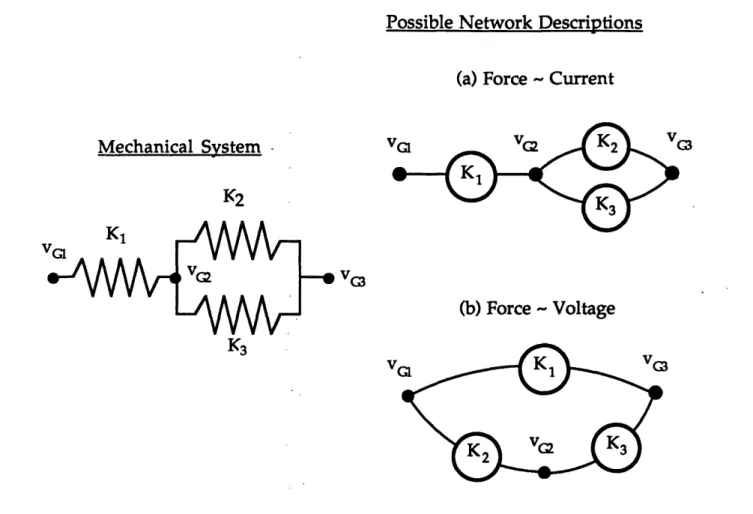
be imposed on the system. These concepts can be demonstrated with a simple structural system in Figure 2.1:

Mechanical System Network Description

zi

'lmon,

1

I I

Port 1

Figure 2.1 Network Description of a Simple Mechanical System

This single degree of freedom (DOF) system can be modelled as having 2 nodes, and 3 branches. The 3 branches are composed of 2 elements and 1

port. It is important to note that the structural mass element has been modeled as an element between the moving node, vG1, and the ground node,

vGo. All masses are modelled as elements to the ground node. This is due to the dependence of inertial force on the absolute acceleration of the mass.

The two structural members, the mass and the spring can be thought of

as two branches of a network between the moving node, vG1, and the fixed node, vGO. The applied force is represented by another branch through which

an external force acts between the nodes. It is said that the system has a port through which F acts.

- 04"A

;01; K,

ml va

In such generalized networks, every branch has two attributes known as the through and across variables of the branch. In mechanical systems these are the force that acts through the branch and the velocity that exists

across the branch. Thus, in mechanical systems, force is the through variable

and velocity is the across variable. The sign conventions are such that the product of the force and velocity in an element is positive when work is being done on the element. The positive velocity across the element is usually associated with an increase in some physical dimension of the element but

can be an arbitrary assignment. The positive force assignment is made in accordance with the power flow convention and the velocity assignment. For ports the power flow convention will for now be taken as for elements. This

means that the product of force and velocity is defined to be positive when work is being done on the port.

In electrical systems the through variable is commonly taken to be the

current, and the across variable is taken to be the voltage. This establishes a correspondence between electrical and mechanical systems that can be stated:

Variable Mechanical Electrical

Through Force Current

Across Velocity Voltage

This convention is one of the two commonly used in comparing the behavior of electrical circuits and mechanical systems, the other being the comparison of force with voltage (the "effort" variables) and velocity with

current (the "flow" variables) as in Paynter [9]. Purely from the perspective of

comparing differential equations, both conventions are valid analogies. But as is shown in Fig. 2.2, the correspondence used here preserves both the dynamic behavior and the topology of the network, and is used in such

general discussions of system dynamics as Penfield, Ref. [6], and Cannon, Ref. [7]. By choosing the through/across correspondence the rules for mechanical

network reduction follows the same rules as those more widely known for

electrical networks. This correspondence will be explained and exploited in a

Possible Network Descriptions

(a) Force - Current

Mechanical System

-VG3

(b) Force - Voltage

K3

V(

Figure 2.2 Possible Network Descriptions of a Simple Mechanical System Showing the Networks Which Result from Comparing Force to Current (a) or Voltage (b)

2.2.2 Force Equilibrium and Displacement Compatibility

'There are constraint conditions that apply among the through and

across variables. As demonstrated in Ref. [10], these constraints are known as

force equilibrium at the nodes and displacement compatibility for the branches in mechanical systems. In electrical systems, they are known as

Kirchoff's current and voltage laws respectively.

Force equilibrium is the statement that all the forces acting on a node

must sum to zero. This is true because inertial reactions have been represented by D'Alembert forces acting through the mass elements. Force equilibrium corresponds to Kirchoff's current law in electrical systems, and the mathematical expressions of these constraints are identical. For

(3 I

mechanical systems, force equilibrium can be expressed by defining the vector

which contains the forces in all the branches (elements and ports) known as

the Branch Force Vector, Fa, in terms of a set of independent forces in the Independent Force Vector, Fi.

Fa = BPF (2.1)

Where Fa is the Branch Force Vector, and Fp is the Independent Force Vector.

The matrix, B,p called the loop matrix in electrical circuit analysis, defines the relationship between the independent and dependent forces. The independent force vector can be composed of any group of port or element

forces which are not linearly related.

The number of independent forces can be found from network analysis

(Ref. [6]) to be:

a =b -nt+ s (2.2)

where a is the number of independent forces, b is the number of system branches (elements and ports), nt is the number of system nodes, and s is the number of separate networks. The loop matrix, B, has the dimensions b by a.

The loop matrix is very useful in network analysis. An example of system analysis where the loop matrix is derived is shown in Section 2.8. As can be

seen, it is directly attributable to the linear relationships which exist among any system with redundant load paths.

The second constraint on the network variables is velocity

compatibility. In mechanical systems, it is the statement of the geometric constraints of the system: that all the branches connecting two nodes must have the same velocities across them. It's electrical analogy is Kirchoff's

voltage law. Mathematically, velocity compatibility can be expressed:

T

BaPVa = 0 (2.3)

Where B is found to be the same loop matrix as was used in the statement of force equilibrium (Ref. [6]). These two expressions for force equilibrium and

displacement compatibility, (2.1) and (2.3), can be combined to derive Tellegen's Theorem

2.2.3 Tellegen's Theorem

Tellegen's Theorem is a convenient expression for the force and velocity constraints on a system. Pre-multiplying equation (2.1) by vaT we obtain:

VTFa =VTB F (2.4)

This can be simplified by noting that the right hand side of (2.4) is zero due to (2.3). This reduction gives the simplest form of Tellegen's theorem.

vTFa = 0 (2.5)

Equation (2.5) represents a summation over all the network branches. The branches can be divided into elements and ports. The ports can be separated out to the right hand side of (2.5) leaving the summation over the

elements on the left. The sign convention for the ports will also be changed so that now the product is positive if the port is doing work on the remainder of the system. This yields:

veTFe = vTFp (2.6)

Where the subscript, e, represents the system elements; and the subscript, p, represents the system ports. This equation represents summations over the elements and ports of the system and relates the work done by the ports on

the system to the work done on the elements within the system.

Equation (2.6) can be generalized by introducing linear operators to act

on the forces and velocities. A justification for this generalization is

presented in Ref. [6]. The linear operators acting on the forces must be the same for all the forces and the linear operators for the velocities must be likewise the same for the velocities though not necessarily the same as those

for the forces. Some allowable operators are: integration, differentiation, multiplication by a constant, Fourier or Laplace transforms, and complex conjugation. By applying the linear operators to Equation (2.6) the general

form of Tellegen's Theorem is obtained.

AV vTAFFe= AVp AFFp (2.7)

This equation exhibits several properties useful for the analysis of systems obeying the force and velocity constraints. The first property is a result of the fact that nowhere in the derivation of the equation was it assumed that the forces and velocities belong to the same load case. Thus

forces and velocities from unrelated applications can be used to satisfy

Equation (2.7). The consistent elemental forces from some arbitrary loading

case can be combined with the consistent velocities from some unrelated loading. When that unrelated load is applied at a node where the velocity resulting from a complex loading are desired, this technique becomes the dummy load method of elementary structural analysis as presented in Ref.

[10]. Being able to use unrelated cases can simplify the analysis of a system greatly.

Another property arises from the fact that none of the constitutive properties of the elements have been included in Equation (2.7). The only required common point between the loading and velocity cases is that they

are from networks with the same topology and therefore have the same loop

matrix. Tellegen's Theorem is based on network properties and is

independent of the type of elements which make up that network. The actual

makeup of the network from which the consistent forces are taken and the

network from which the compatible velocities are taken need not be similar. Dampers in the network to which the forces belong can be replaced by-springs

in the network to which the velocities belong. Nonlinear elements can be

replaced by linear ones and Equation (2.7) will still hold. This property opens

options for system analysis and has been applied fruitfully to electrical

systems.

Since the constitutive relations for the elements were not used in the derivation, Tellegen's Theorem is valid for arbitrary systems including structures with time varying, non-linear, and frequency dependent elements. In fact it is frequently used to analyze electrical systems with nonlinear capacitors or transistors as elements. For these systems it can be used to establish bounds on the energy that is transferred to higher harmonics by

nonlinear elements (Ref. [11]). In this report, advantage will be taken of this

property to model and analyze the energy dissipation characteristics of

systems with frequency dependent elements or subsystems.

Specializing the general statement of Tellegen's Theorem, Equation

(2.7), by using the Laplace operator on the forces and velocities, a frequency domain expression for Tellegen's Theorem can be obtained. Letting Av select the complex conjugate of the Laplace transform and AF select only the Laplace transform, Equation (2.7) becomes:

V .() ='(s)Fp(s) (2.8)

Where the tilde, ~, represents the Laplace transformed variable. From this

point forward all forces and velocities will be in the frequency domain and the tilde will be omitted for simplicity.

If we consider the system to be operating in sinusoidal steady state (s =

io), then the Laplace transform can be thought of as the Fourier coefficients representing the amplitude and phase of the sinusoidal signal. Throughout the rest of the report, the Laplace transformed variables will be used. The

explicit dependence on the Laplace variable, s, may be omitted for simplicity but the frequency dependence will be implicit.

2.3 Structural Impedance and System Modelling

At this point the relationships for the topology, ie. displacement compatibility and force equilibrium, have been expressed by Tellegen's Theorem; and it is desirable to introduce the constitutive relations for the

individual elements. Since Tellegen's Theorem will be employed in the frequency domain, the constitutive relations will be introduced by using the

frequency dependent ratio of the velocity and force to eliminate the elemental

forces from Equation (2.8). The equations will then be converted from elemental to global coordinates to give the system equations in their final form.

In a mechanical system various names are given for the ratio between the force in a system and various output variables. These names from have been compiled by Ewins [12] and presented in Table (2.1). In this report, the concept of mechanical impedance will be utilized for system modelling and analysis since it relates the force and velocity in a system element. It is expressed as the ratio of the Laplace transformed force over the Laplace transformed velocity. For nonlinear systems, it may be amplitude dependent.

The mechanical impedance for a mass, spring, and damper are:

ZM(S) = M s (2.9a)

Response Parameter R/ F F / R R

Receptance,

Displacement Admittance, Dynamic Stiffness Compliance

Mechanical

Velocity Mobility

Impedance

Acceleration Inertance, Apparent Mass

Accelerance Apparent Mass

Table 2.1 Possible Frequency Domain Constitutive Properties

Zc(S) Ks (2.9c)

The impedance can be a more complicated function of frequency as in

the case with elements with resonant subsystems or viscoelastic behavior. For general elements with connections to more than 2 system nodes the

concept of a impedance matrix can be used to relate the forces and velocities

associated with the element. Thus in general for the linear elements, the constitutive relations can be written

FL (S) = ZL(S) VL (S) (2.10)

where FL is the vector of linear elemental forces, VL is the vector of linear

elemental velocities and ZL is the linear elemental impedance matrix.

The elemental impedances can be substituted into equation (2.8) to

eliminate the explicit reference to the forces of the linear elements.

V HZLV L+ NL FNL Fp (2.11)

A few moments should be taken to examine the structure of Equation

(2.11). The system described above will be defined to have b branches where b

is the sum of the number of linear elements, n, the number of nonlinear elements, m, and the number of ports, k. The first term on the left is a summation over the linear elements of the systems. For a system with n linear elements, it can be represented

-ZL1 . . .

. ZL2

[VL 1 VL2 "' VLn*.

o . . . ZLI

Where the superscript, *, represents the complex conjugation. The elemental impedance matrix is diagonal; and, when pre and post multiplied by the elemental velocities, it represents a summation over the linear elements of

the system. The second term of (2.11) can be represented as a summation

over m non-linear elements

[VNL 1 NL 2 . . VNL m NLF N H FN (2.13)

NL

Likewise the third term can be represented as a summation over k system ports

[V 1 vp2 . . . vp k F 1- =v HF (2.14)

These summations can be condensed and simplified if it is noted that

the elemental velocities, the relative velocities across the elements, can be represented as linear combinations of the absolute velocities of the system nodes relative to inertial space. The velocities at the nodes will be called the

global velocities which exist in the inertial frame in the global coordinate system of the nodes. Fist a transformation between the global "point"

velocities and the elemental "across" velocities must be defined. The velocity across the element can be thought of as the difference between the velocities

of the nodes of that element after an appropriate coordinate rotation. Thus a transformation matrix can be defined:

vp Tp

VL = TL VG=TvG (2.15)

VNL T

-where VG is the vector of absolute nodal velocities and vp, VL and VNL have

been previously defined. The various partitions of the transformation matrix, T, can be used to convert the elemental forces and impedances of Equation (2.11) into more easily conceptualized point forces and impedances.

Substituting the appropriate partitions of (2.15) into (2.11) gives us Tellegen's

Theorem in terms of point quantities

VHZ _{G G} VG + VHFN _{G G-NL} = HF _{G G-P} (2.16)

where:

FGp = TP Fp (2.17a)

FG =T FNL (2.17b)

ZGL = TLZ LT L (2.17c)

Tellegen's Theorem is now in a form dependent only on the velocities of the nodes, the global impedance matrix, ZG-L, which contains the elemental

constitutive relations in the global coordinate system, and the forces due to the ports and nonlinear elements. At this point either the driving forces or

the nonlinear forces could also be eliminated by defining the appropriate port or non-linear impedance matrix. For the nonlinear elements, the forces can be described by state dependant impedances

FGNL = ZGNL(VG, 'S) VG (2.18)

This nonlinear impedance can be used to replace the nonlinear forces in Equation (2.16) to obtain a global impedance matrix for the system.

VH Z S) VG =V v FG.P (2.19)

were:

The size of the resulting frequency domain system matrix might be

quite large for a system with many degrees of freedom. There are, however,

many techniques for reducing the sometimes cumbersome size of the global

impedance matrix. The ones described here are drawn from techniques used

for reduction of discrete time domain models. The first and probably most useful is the elimination of degrees of freedom with no external forcing at them by using static condensation on the global impedance matrix. Static condensation is usually employed in the reduction of system stiffness matrices and is customarily thought of as a quasi-static condensation for dynamic systems. If, however, the frequency dependant system impedance matrix is reduced using this method then the reduction is an exact dynamic reduction since the mass information is included in the impedances. The equations for the static condensation technique can be found in Ref. [13]. When the impedance matrix is reduced, a lower order but more complicated frequency dependent matrix is the result. This matrix contains all the information inherent to the larger model and the condensed information can

be recaptured if necessary.

The second reduction method is the assumed mode technique. The

global set of degrees of freedom is reduced to a smaller set of generalized coordinates by assuming a linear relation among the global set. An example of an application of this method is the assumption of rigid body motion for

some set of the boundary nodes or a conversion to modal coordinates

common in dynamics. This type of reduction is not guaranteed to be exact but

can result in problem simplification. It usually does not greatly complicate the frequency dependence of the impedance matrix. These two techniques

can be used to great advantage in complex system reduction and analysis.

2.4 Comparison of Tellegen's and Hamilton's Theorems

A version of Hamilton's Theorem can be derived from Tellegen's Theorem for discrete systems. The derivation serves to highlight the relationship between the various power products in Tellegen's Theorem and the conventional kinetic and potential energies. The derivation will also help place Tellegen's Theorem on more familiar ground for system

operators in the general form of Tellegen's Theorem. If we recall the form of

the theorem presented in Equation (2.5):

vtaFa = 0 (2.21)

This form of Tellegen's Theorem has not yet been specialized to the frequency

domain by use of the Laplace operator nor have the branches been separated into elements and ports by the sign convention. This form of Tellegen's

Theorem represents a summation over all the branches of a system.

The coordinate system of Equation (2.21) can be transformed from

elemental to global using the transformation technique outlined in the

previous section for Equation (2.15). The equation can also be generalized just as was Equation (2.7) to allow operators on the forces and velocities. The result is a generalized product of the nodal forces and velocities of the system.

A -V· AFFG=0 (2.22)

Any linear (and some nonlinear) operator or sets of operators may be chosen as the A's of Equation (2.22) as is explained in the appendix of Ref. [6].

If Av is defined as the variational of an integral with respect to time then

Equation (2.22) becomes:

SxAFFG = (2.23)

Furthermore, taking the transpose of (2.23) and integrating from t to t2, a

variational equation emerges:

[FSXG]dt = (2.24)

ti

At this point it is necessary to consider the makeup of the nodal forces. The global force vector, FG, represents at each degree of freedom the sum of the elemental forces (for elements such as masses or stiffnesses) as well as the externally applied forces at that particular degree of freedom. It is convenient

to divide the global force vector into its component parts: the conservative

forces such as spring forces or gravitation; the inertial forces due to the mass

elements; and the non-conservative forces arising from energy dissipation

t2

FIN SXG + FTO BX_G + FNCXG] dt = (2.25) tl

Each of these groups of terms has a specific relationship to the energy

in the system. The inertial forces relate to the kinetic energy and the

conservative forces relate to the potential energy. To determine exactly how

these terms relate to their respective energies, variational calculus must be

employed. If we assume that the conservative force can be associated with a

possibly time varying stiffness matrix and that the inertial force or

D'Alembert force can be associated with a mass matrix, we can obtain:

[- G(t) xG, G( = -U=- (2.26a)

[-MG(t),o']TxG =± 2 [M()] = (2..26b)

Substituting these expressions into Equation (2.25) and separating out the

non-conservative part gives us the well-known form of Hamilton's Principle:

8[T

t1 ti

Thus, a version of Hamilton's Principle for discreet dynamic systems

can be derived from Tellegen's Theorem. The subtlety is in the choice of

appropriate linear operators to be used in the general form of Tellegen's Theorem and in the recognition of the various contributions to the nodal

forces.

Many other variation expressions for dynamic systems can be developed by starting with the general form of Tellegen's Theorem and using alternate linear operators. In this work, the Laplace transform was chosen, which has the effect of transforming the system equations into the frequency domain. The choice of the linear operator in no way affects the amount of information about the system that is contained in the equations. The frequency domain representation of dynamic systems thus contains the same fundamental information as the more common Hamilton's Principle and is equally valid for dynamic systems.

2.5 Conservation of Real and Reactive Power

In this section an attempt will be made to determine the nature of the

energy expressions inherent in the frequency domain statement of Tellegen's

Theorem. In Equation (2.8) both the force vector and the velocity vector for

the elements and the ports have real and imaginary parts. The product of

force and velocity is power. This product can also be divided into real and

imaginary parts. The real part is termed the real power, and the imaginary part is termed the reactive power. Since the force/velocity product must be equal for the ports and the elements, Tellegen's Theorem in the frequency domain is sometimes referred to as the conservation of real and reactive power.

Power is a time domain quantity and is calculated from the time domain product of the instantaneous force and velocity. The terms of

Equation (2.19) are frequency domain products. Strictly speaking, the Laplace

transform of the time domain power would involve a convolution integral of the transformed force and velocity since time domain multiplication corresponds to frequency domain convolution. Therefore the product of the transformed force and velocity does not represent the Laplace transformed instantaneous power but rather some related quantity. The nature of this

relationship will be examined in the following section.

Two approaches will be taken to gain insight into the frequency domain product of force and velocity. First a relationship will be derived between the average energy dissipated in the elements during a cycle and the

real part of the frequency domain product of force and velocity. In the second

approach, a simple form will be assumed for the mechanical impedance and the resulting contributions to the real and reactive power will be analyzed.

The forms of these contributions will be related to system energy terms and

used to derive approximate formula for system natural frequencies and loss

factors.

To begin the analysis of the physical significance of the real and imaginary parts of the frequency domain system model proposed in Equation

(2.19), the various contributions of the terms of (2.19) to the real and reactive

power must be determined. Multiplying Equation (2.19) by a half and dividing the products into their real and imaginary parts, Equation (2.19) can

(PP +iX) =(PE + iXE ) (2.28)

where Pp and Xp are the real and imaginary parts of:

P+ iX Re{ V FGP} + i Im{ V FP} (2.29) and PE and XE are the real and imaginary parts of:

PE E=Re{= 2 G G(V HH )v + i m{ ZG(v, s)V } (2.30)

These terms are all frequency dependant; and in the case of the system

impedance matrix, they can be amplitude dependant also.

At this point, it is desirable to gain some physical insight into the source of these frequency domain power terms. To make this easier, some simplifying assumptions will be made for the system in Equation (2.28). It

will be assumed now that the system is in steady state and the complex forces and velocities of Equations (2.28) to (2.30) represent the magnitude and phase

of sinusoidal signals. It will also be assumed that the system is linear and reciprocal. This means that the system can be represented by a symmetric

impedance matrix. This assumption will not limit the derivations

applicability for damped structural systems since systems with material

damping or internal resonances still maintain reciprocity.

We will examine the time domain expression for power dissipated in a cycle first and relate this to the real part of the frequency domain product, PE. The forces due to the system elements can be represented as a function of the

system velocity vector and the system impedance matrix using Equation

(2.10). For a linear system being forced at frequency, o, this frequency domain force can be expressed in the time domain

FG.L(t) = FR coscot + FIsincot (2.31)

and likewise the velocity can be expressed

VG(t) = VR coscot + vI sincot (2.32)

Using these time domain expressions for the elemental forces and velocities,

the energy dissipated in the elements in a cycle of period T would be written: T

Edi = J[T(t) F(t)]dt (2.33)

When evaluating the integral, the terms containing a product of sine and cosine integrate to zero leaving only terms with squares of sines or cosines.

These terms integrate to 1/2 T over one cycle leaving

Eds

1T.F

vT.

1 HF

= = + I I = real G -L (2.34)

Since F can be expressed in terms of the impedances of the system and its

velocities, Equation (2.34) can be put into a quadratic form for the average

power dissipation in a cycle

T= Real ,2 vGs)G (2.35)

The right hand side of Equation (2.35) is identical in form to the first term on

the right hand side of (2.30). Therefore we can conclude that for linear systems

Ed.is

PE PP T (2.36)

Thus the real part of the product of the Laplace transformed forces and velocities is numerically equal to the average power dissipation in a cycle. This explains why this term is named the real power when in fact its relation to that time domain quantity was not obvious. This frequency domain expression for energy dissipation will be used in developing an approximate

method for calculating the system loss factor in the next section.

Equation (2.35)'s validity for nonlinear systems is limited to the degree

that the elemental forces and velocities can be expressed as simple phase shifted sinusoids with a single frequency component. If the nonlinearities introduce higher order harmonics or other coupling which results in a more complex time history, then Equation (2.32) and consequently (2.35) are not

strictly valid. If however the nonlinearities introduce only small

perturbations to the otherwise linear response, then Equation (2.35) can be

said to be approximately valid.

The nature of the complex part of the product, XE, is more subtle. It

represents the product of the forces and velocities that are in quadrature. These power terms integrate to zero over a period of the system, although the

The physical significance of the reactive power will be interpreted in

terms of the contributions from the real and imaginary parts of the system

velocity vector and impedance matrix. As before, the system will be assumed

to be linear and reciprocal. A simple dynamic system impedance model will

be assumed in order to relate the components of the reactive power to kinetic and potential energies. First, the real and reactive power in the elements can be expressed for general systems in terms of the quadratic form involving the

system impedance matrix:

+ iXE ,GHZV G 2 V i (ZR+ iZXVR + i 1 ) (2.37) expanding,we obtain +VTz - VTZv +VTZRV

(2.38a)

3

P = V ZR VTR + ZR VI) (2.39a)

XE =(vT ZI VI + R ZI yVR ) (2.39b)

Notice that PE and XE involve only the real and imaginary parts of the global

impedance matrix respectively. This leads to some conclusions concerning

damping in structural systems. Since, by (2.36), PE is equivalent to the

average power dissipation in a cycle, we discover that the system's energy dissipation at a particular frequency is dependant on two factors, the size of

the real portion of the system impedance matrix and its placement in relation

to the system modeshape at that frequency. Both factors are important in maximizing the energy dissipation product in (2.39a).

At this point a form for the system impedance matrix must be assumed in order to gain further insight into the nature of the reactive power. Although the actual system impedance can be a complicated function of the complex frequency, within a narrow frequency band the complicated

expressions can be represented with varying degrees of accuracy by a simple impedance model containing equivalent mass, stiffness, and damping matrices. In this simple structural model, the global impedance matrix has

the form:

(S) =ZR(S)+iZI(s)= C +(Ms + ) = C + i0M (2.40)

where C is the equivalent damping matrix, M is the equivalent mass matrix,

and K is the equivalent stiffness matrix. Substituting Equation (2.40) into the expression for real and reactive power, Equation (2.39) leads us to several

conclusions. The first is that the real power dissipated, PE, depends solely on

the complex modeshape and the equivalent system damping matrix, C. With a more general form for the impedance, the dissipated power could also depend on any complex part of the mass or stiffness matrix. These complex parts can result from the complex modulus representation of material

damping or viscoelastic materials or from internal system resonances. They

contribute to the real part of the impedance matrix and thus to the power

dissipation as is demonstrated in equation (2.39).

Secondly, the reactive power in the elements, XE, is a function of the effective mass and stiffness matrices and the complex velocity modeshapes. This dependence on the mass and stiffness matrix is of a very specific form. If

the system modeshapes are assumed to be primarily real, then the first term

of Equation (2.39b) can be neglected and

1 T TV

VXE=±v

ZvvR(4MV vR V 2RJ (KE PE) (2.41a)

X2 L E- (2.41b)

Where L is the well-known system Lagrangian. So for linear, reciprocal

systems which can be represented by the effective impedance of the form of

Equation (2.40) and which have predominantly real modeshapes, the

imaginary reactive power represents the average difference between kinetic

and potential energy at a given frequency. Systems with predominantly real modeshapes are those with symmetric matrices and light damping. For systems with very complex modeshapes (ie, highly damped) the definitions of

the energy either potential or kinetic. This is the result of different parts of the structure being out of phase with each other in very complex

modeshapes. Expression (2.40) will be used to derive the effective mass and stiffness matrix for a frequency dependent system as will be shown in Section

2.6

At this point the quadratic product of the frequency dependent modeshapes and the system impedance matrix has been analyzed and understood in terms of the energies in predominantly linear, lightly damped,

reciprocal systems. For such systems, the quadratic expression can be written:

IV HZV = (Edis + i2rL (2.42) This compact form is very useful in determining properties of the system such as modal frequencies and loss factors as will be discussed in the next

section.

2.6 Quadratic Approximations of Frequency and Loss Factor

In this section approximate methods for calculating natural frequency and damping from the global impedance matrix will be developed. These methods involve using approximate mode shapes in a manner similar to the way in which they are used in the Rayleigh Quotient for natural frequencies. These forms can be very useful for finding approximate poles of a system, since finding the exact poles for the frequency dependent system can be

difficult (These difficulties are outlined by Anderson in Ref. [14]).

In general a natural mode of the system occurs when the determinant

of the impedance matrix equals zero, Ref [15].

ZG(s) =0 (2.43)

The process of finding the values of s in the complex plane is complicated by

several factors and usually requires a numerical procedure. The procedure used in this report is presented in Appendix A, Section A.4. One

complicating factor is that Z is very often a complicated, non-linear function

of the complex frequency, s. It can involve transcendental expressions or other nonlinear forms. Another complicating factor is that for higher order

and thereby cause computational difficulties. In the exact calculation of the

eigenvalues of the system, a good approximate initial value helps to circumvent these difficulties. In this section, expressions will be derived for

these approximate values.

One common way of finding the approximate natural frequencies of an undamped system is to employ the Rayleigh Quotient, Ref. [16]. The quotient

is expressed as the ratio of two quadratic forms, that of strain to reduced

kinetic energy:

1T

i

e

(2.44)

T21 MGC

In practice, it makes no difference whether displacement or velocity

modeshapes are used in (2.44) since in steady state the frequency constant will

cancel out. Thus (2.44) can equally well be written in terms of velocity modeshapes:

Re(- G ) (2.45)

2G

Re(ivTM _2G v)_{G G}

and corresponds exactly to the condition that the L in Equation (2.41b) equals zero.

Now we are going to try to find a way to calculate the stiffness and mass

matrices used in (2.45) from the system or elemental impedance matrices.

This method is also presented in Appendix A. The impedance matrix is a complex, non-linear function of frequency which can be obtained from a simple dynamic test of a structure, whereas the stiffness and mass matrices for

complicated sub-structures with internal resonances or frequency varying

properties are sometimes difficult to model. The goal is to derive a simple

method for finding the equivalent system stiffness and mass matrices for systems which contain elements with frequency variable properties and high

damping. This method will also be useful in analysis of lower order system

models which contain resonant subsystems due to the reduced out degrees of freedom.

One way to accomplish this is to assume that in a given frequency range the system impedance matrix can be modelled using equivalent mass,