Detecting, Tracking, and Warning of Traffic
Threats to Police Stopped Along the Roadside
by
James Karraker
Submitted to the Department of Electrical Engineering and Computer
Science
in partial fulfillment of the requirements for the degree of
Master of Engineering in Electrical Engineering and Computer Science
at the
MASSACHUSETTS INSTITUTE OF TECHNOLOGY
June
2013
@
Massachusetts Institute of Technology 2013. All rights reserved.
Author...
..
...
...
Department of Electrical Engineering and Computer Science
May 23, 2013
Certified by...
...
Seth Teller
Professor
Thesis Supervisor
Accepted by...
.n
Prof. Dennis M. Freeman
Chairman, Masters of Engineering Thesis Committee
Detecting, Tracking, and Warning of Traffic Threats to
Police Stopped Along the Roadside
by
James Karraker
Submitted to the Department of Electrical Engineering and Computer Science on May 23, 2013, in partial fulfillment of the
requirements for the degree of
Master of Engineering in Electrical Engineering and Computer Science
Abstract
Despite years of research into improving the safety of police roadside stops, reck-less drivers continue to injure or kill police personnel stopped on the roadside at an alarming rate. We have proposed to reduce this problem through a "divert and alert" approach, projecting lasers onto the road surface as virtual flares to divert incoming vehicles, and alerting officers of dangerous incoming vehicles early enough to take life-saving evasive action. This thesis describes the initial development of the Officer Alerting Mechanism (OAM), which uses cameras to detect and track incoming vehi-cles, and calculates their real-world positions and trajectories. It presents a procedure for calibrating the camera software system with the laser, as well as a system that al-lows an officer to draw an arbitrary laser pattern on the screen that is then projected onto the road. Trajectories violating the "no-go" zone of the projected laser pattern are detected and the officer is accordingly alerted of a potentially dangerous vehicle. Thesis Supervisor: Seth Teller
Acknowledgments
This work is partially funded by the National Institute of Justice. Any opinions, findings, and conclusions or recommendations expressed in this thesis are those of the author and do not necessarily reflect the views of the National Institute of Justice.
Professor Seth Teller, for giving me this wonderful opportunity to work on a great project with life-saving potential.
Professor Berthold K. P. Horn, for his invaluable help with the machine vision al-gorithms and all the math behind them.
Brian Wu and Pallavi Powale for being great teammates on the project, and putting up with me in the lab.
Contents
1 Introduction 8
2 Background 10
2.1 Review of Relevant Literature ... ... 10
2.1.1 Incidence of Roadside Accidents . . . . 10
2.1.2 Lane Estimation . . . . 11
2.1.3 Vehicle Tracking and Classification . . . . 11
2.2 LCM ... ... ... ... ... 12
3 Problem Statement 13 3.1 Officer Alerting Mechanism (OAM) . . . . 14
3.1.1 Sensors and Geometry . . . . 14
3.1.2 Vehicle Detection . . . . 15
3.1.3 Vehicle Tracking . . . . 16
3.2 Sensor Calibration . . . . 16
4 Technical Achievements/ Steps 18 4.1 Assumptions . . . . 18
4.2 Vehicle Detection and Tracking . . . . 19
4.2.1 Detection . . . . 19
4.2.2 Tracking Headlights . . . . 20
4.2.3 Headlight Pairs . . . . 21
4.3.1 4.3.2 4.3.3 4.4 Laser 4.4.1 4.4.2 4.4.3
Vision Algorithms to Recover Road lines Software System To Recover Road Lines Position and Velocity Calculation . . . .
Calibration . . . . Homography . . . . Galvanometers . . . .
Calibration Software System . . . .
5 Results and Contributions
5.1 Results . . . . 5.1.1 Specifications . . . . 5.1.2 Performance . . . . 5.1.3 Lane Characterization . . . . 5.2 Contributions . . . . 5.3 Future Work . . . .
5.3.1 Vehicle Detection and Tracking . .
5.3.2 Headlight Pairing . . . .
5.3.3 Characterizing Dangerous Vehicles 5.3.4 User Interface . . . .
5.3.5 OAM Performance Evaluation . . . A Setup Instructions
A.1 Checkout the Repository . . . . A.2 Run the Headlight Tracker Code . . . . A.3 Run Laser . . . .
A.4 Run Alert code . . . .
B Code . . . . 2 2 . . . . 26 . . . . 2 6 . . . . 2 8 . . . . 29 . . . . 35 . . . . 3 9 46 . . . . 4 6 . . . . 4 6 . . . . 4 6 . . . . 4 7 . . . . 4 9 . . . . 50 . . . . 50 . . . . 5 1 . . . . 5 2 . . . . 5 3 . . . . 53 54 . . . . 54 . . . . 54 . . . . 55 . . . . 55 56
List of Figures
1-1 A conceptual illustration of the Divert and Alert system usage case. 9
3-1 Short and long exposure images of the road. . . . . 16
4-1 A zoomed-in image of the tracker code. . . . . 20
4-2 A diagram of the camera and the road showing coordinate frames. . . 23
4-3 The road lines program running on the log from a ride along. . . . . . 27
4-4 The user can toggle the level of the road markings. . . . . 28
4-5 The road lines program after integration with the tracker . . . . 29
4-6 The relationships between the camera, laser, and world coordinate sys-tem s. . . . . 30
4-7 The coordinate system for the galvanometers. . . . . 36
4-8 Step 1 of the laser calibration process. . . . . 40
4-9 Step 2 of the laser calibration process. . . . . 41
4-10 Step 3 of the laser calibration process. . . . . 42
4-11 Step 4 of the laser calibration process. . . . . 43
4-12 Step 5 of the laser calibration process. . . . . 44
4-13 A demo of the laser calibration procedure. . . . . 45
5-1 The group testing the laser and camera systems at the BAE facility in M errim ack, NH. . . . . 47
List of Tables
Chapter 1
Introduction
Police officers and their vehicles are frequently struck by incoming drivers while stopped along the roadside. Despite regular use of vehicle mounted emergency light-ing (VMEL) systems to alert incomlight-ing drivers, there are a regrettably high number of injuries and deaths caused by impaired drivers. Other drivers are apparently not impaired, yet still do not notice or react to the police officer on the side of the road. This leads us to believe that existing VMEL systems fail to generate sufficiently ef-fective cues to divert incoming vehicles. Some drivers, however, are indeed impaired, in which case no type or amount of emergency lighting may divert that driver from colliding with the officer. In this case an easy-to-deploy mechanism is needed for alerting the officer of an incoming potentially dangerous vehicle, early enough so that the officer has enough time to get out of harm's way.
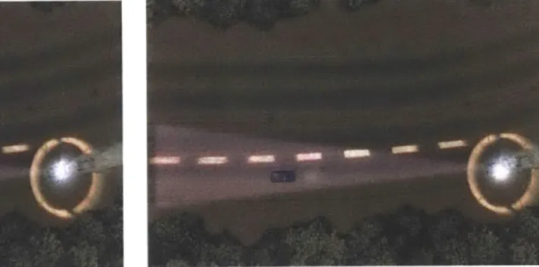
To solve these two main problems and reduce the number of these preventable ac-cidents, we use a two component approach: divert and alert. Our Motorist Diverting Mechanism (MDM) projects virtual flares onto the road using lasers, giving incoming drivers visible cues to change course and avoid the officer and parked police vehicle. Our Officer Alerting Mechanism (OAM) detects incoming vehicles and determines if they are potentially dangerous, in which case it alerts the officer of the danger so that he or she can take evasive action. Figure 1-1 shows an example of the environment in which the system would be used.
Sensor Networks group (RVSN), BAE, and the Massachusetts State Police. This
the-sis will focus mainly on the OAM, and the detection, tracking, and machine vision
algorithms that have gone into it. Section 2 reviews relevant background material.
Section 3 states the problem. Section 4 provides an overview of the technical
achieve-ments I have made and detail the steps I have taken in my work on the OAM. Section
5 evaluates some results of my work, analyze my contributions to the project, and
present opportunities for future work.
(a) A police cruiser parked on the roadside (b) The system detects when an incoming ve-looks back at the road and projects a line of hicle breaks the flare line and presents a dan-laser virtual flares. ger to the officer, then alerts the officer early
enough to take life-saving evasive action.
Figure 1-1: An example of the Divert and Alert system usage case. The dotted lines
are laser virtual flares, and the pink cone represents the camera's field of view.
Chapter 2
Background
2.1
Review of Relevant Literature
In this section I will perform a brief review of literature relating to roadside accidents,
lane estimation, and vehicle tracking.
2.1.1
Incidence of Roadside Accidents
Roadside accidents involving police officers are relatively well documented. I will
highlight some interesting statistics that have come out of the documentation on
these types of accidents. The most recent findings show that over the decade from
2000-2009, there were 47 law enforcement officer deaths from being struck by a vehicle
while conducting a "Traffic stop, road block, etc." in the United States. Another 73
deaths occurred while the officer was "Directing traffic, assisting motorist, etc" [21].
Solomon and Ellis (1999) found that most roadside incidents with police vehicles
occur on straight, dry roads in clear weather[17]. Charles et al. (1990) found that
the normative condition for roadside accidence involved unimpaired drivers, and that
the majority of accidents occurred on unmarked roads[3]. They also found that the
number of roadside accidents with police vehicles was proportionally similar to the
number of accidents with passenger vehicles. In addition they found that a common
cause of the accidents is sleep deprivation. Agent and Pigman (1990) also found that
sleepiness, as well as alcohol impairment, were major causes of roadside accidents[1]. These results seem to suggest that there are many accidents that no diverting system can prevent because the driver is so insensate due to impairment or sleepiness. In these cases a warning system would be the only effective way to avoid injury to the officer on the side of the road.
2.1.2
Lane Estimation
Our own group, the Robotics, Vision, and Sensor Networks Group, has developed sensor-based methods for identifying and locating nearby traffic lanes on real roads under challenging lighting and weather conditions[13, 14]. Lane estimation was for-matted as a curve-fitting problem, where local sensors provided partial, noisy ob-servations of lane geometry. The system can handle roads with complex geometries without making assumptions about the position or orientation of the vehicle.
Mobileye is a commercially available system that uses monocular vision algorithms to perform lane detection, among other applications. The Mobileye system sits on the dashboard of a moving car, and uses its algorithms to help the driver drive more safely, by giving him or her lane departure warnings, forward collision warnings, and similar features[16]. To our knowledge no lane-finding method specific to roadside vehicles has been developed.
2.1.3
Vehicle Tracking and Classification
An enormous body of work exists on video-based object detection, tracking, and clas-sification. Stauffer and Grimson (1999) created a widely used mixture-of-Gaussians background modeling algorithm that detects moving objects, which works very well for stationary cameras, but cannot handle slight perturbations caused by wind or small vehicle movements[19].
There are also many existing object tracking systems, which either associate in-dividual independent detections over time[5], or search for an object at later times based on knowledge of that object at earlier times[4, 22].
Work in the field of visual surveillance has led to a number of techniques for building normalcy models based on continuous observation[18, 23, 2]. Classification algorithms can use these normalcy models to predict future behavior, such as speed and direction, as well as identify anomalous objects that do not fit the normal behav-ior, such as a swerving car.
2.2
LCM
We use the Lightweight Communication and Marshaling (LCM) protocol to com-municate between separate parts of the system. LCM is a system of libraries for transferring data over a local-area network, which was designed by the MIT DARPA Urban Challenge Team[15]. LCM is made for real-time systems such as ours that require high bandwidth and low-latency data transfer. We have 142 GB of LCM logs (about an hour) of roadside video that we use to test our system. These logs simulate the communication between the cameras and the software system using LCM. We also use LCM to communicate between the laser and the software system.
Chapter 3
Problem Statement
Impaired, inattentive, or sleeping drivers strike police officers and other emergency workers, as well as their vehicles, at an alarmingly high rate, causing damage, injuries, and often fatalities. The traditional way to combat these types of accidents is to alert drivers to the presence of the vehicle on the side of the road in some way. Vehicle-mounted emergency lighting (VMEL) is routinely used to divert drivers from the officers and their vehicles on the roadside. Yet there is still an unnecessarily high rate of accidents, many of them involving apparently unimpaired drivers (Charles et al., 1990)[3]. We therefore conclude that existing VMEL systems fail to generate sufficiently effective cues to divert drivers from collisions with the vehicles on the side of the road.
Some drivers cannot be diverted by any emergency lighting system. In this case, something else must be done to reduce the danger of roadside collisions. We have developed the early stages of an easy-to-deploy mechanism to warn the officer of a potentially dangerous oncoming vehicle, early enough to allow the officer to get out of the way in time to avoid injury.
Our system addresses the problem of roadside collisions from two separate angles, based on the needs we perceive:
1. Create a more effective vehicle-mounted emergency lighting system to divert
2. Create a warning system that robustly perceives potentially hazardous oncom-ing vehicles, and effectively alerts officers in time to avoid disaster.
By combining these two approaches, our system contains two layers of risk mitigation.
The first layer will divert many possibly dangerous oncoming drivers, and the second layer will warn the officer of any vehicles that break through the first safety layer. By integrating these two approaches into a single system we will give police officers and other emergency workers an effective safety net from roadside collisions. I worked on the second approach, the alerting approach, and this thesis will cover that portion of the project.
3.1
Officer Alerting Mechanism (OAM)
The development of the OAM has been focused on writing and evaluating software designed to monitor the roadway behind a stopped police vehicle, detecting oncoming vehicles using machine vision algorithms, evaluating the potential danger of a detected oncoming vehicle, and alerting the police officer of any vehicles deemed potentially dangerous. Research for the alerting portion of the project will consist of evaluating the software system on LCM logs of camera data taken from the roadside during police escorted ride alongs.
3.1.1
Sensors and Geometry
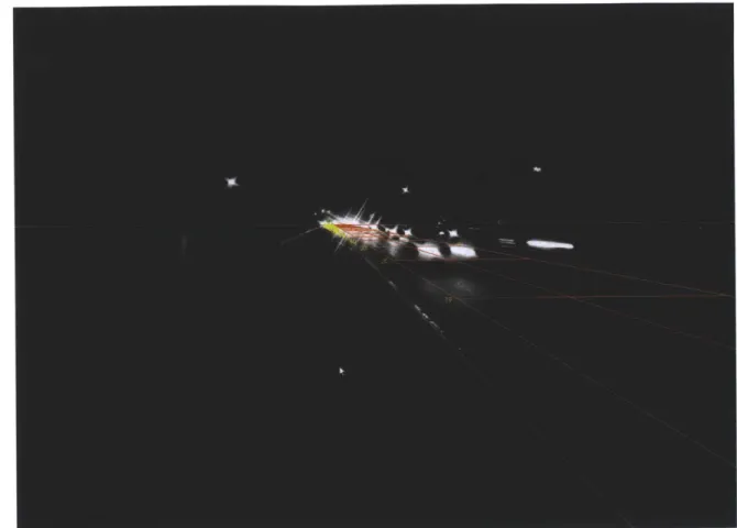
Vision at night is very challenging. Road markings and vehicle bodies are extremely dimly lit, requiring long exposures to show sufficient detail. The long exposure time of the camera causes blur on moving vehicles, which also makes recovering details difficult. Additionally long exposure causes bright objects, such as headlights and streetlights, to saturate the camera and produce a blooming effect. With this bloom, it is very hard to precisely track bright lights. We would like to be able to minimize bloom and track headlights very precisely, but at the same time be able to see details of the road and vehicle bodies.
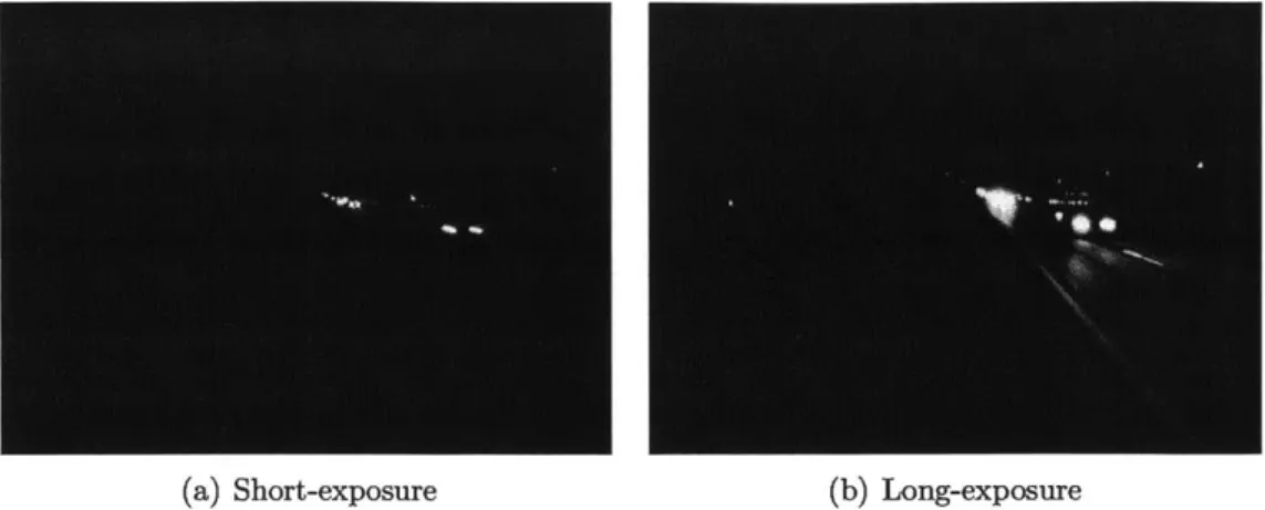
To accomplish these two seemingly contradictory tasks, we mount two identical cameras, one set to short exposure, and the other to a longer exposure. The short exposure camera is set around 1/2000 second exposure time, and is used to detect moving headlights and other bright lights, while minimizing motion blur. The long exposure camera is set around 1/60 second exposure time, and is used to capture details of the road, such as lane lines and other markings, which are stationary and so not subject to motion blur. Figure 3-1 shows the difference between the images from these two exposure settings.
Although we are using two cameras, we are still using a monocular vision approach. The two cameras do not function as a stereo pair, they only differ in their exposures, and are relatively close in position. We do not use a stereo system for three main reasons:
1. We would like the entire system to fit in a small box on top of the vehicle, and a
stereo pair of cameras would require a large distance between the two cameras.
2. Stereo works better the closer the object is to the cameras, but our system is focused on detecting objects at a far distance, and so in this case stereo would not provide much of an advantage.
3. Stereo would require adding at least one more camera, which would bring an
additional cost to the system.
A monocular vision approach implies that we must determine distance in other
ways, such as using assumptions about the shape and size of the road, or assumptions about the height of headlights off the ground.
3.1.2
Vehicle Detection
One of the most critical aspects of the project is the ability to detect and track oncoming vehicles. The task of detection involves recognizing objects as vehicles and determining the precise position of those vehicles. Tracking involves keeping a
(a) Short-exposure
Figure 3-1: Short and long exposure images of the road. Notice the bloom in the long-exposure image, making it very difficult to differentiate headlights in the distance.
consistent representation of each vehicle's position and velocity as it moves through the cameras field of view.
The easiest way to detect vehicles is by looking for headlights. Using the short exposure camera, headlights do not bloom and so can be relatively compact, and so are seen to be distinct from one another. Because the short exposure camera is highly sensitive to bright lights, and dulled to most everything else, it is reasonably simple to detect and track vehicles with their headlights on.
3.1.3
Vehicle Tracking
Once we determine the positions of oncoming vehicles, we form a coherent track for each vehicle by correlating detections over camera frames based on sensor geometry, motion consistency, and proximity.
3.2
Sensor Calibration
We employ three levels of offline sensor calibration. First we estimate camera pa-rameters such as focal length and radial lens distortion, which remain fixed, using a standard procedure[6]. Second we compute the alignment between the two cameras, which remain fixed. Third, we determine a transformation between the cameras and
the laser from the MDM using a sequence of calibration steps built into the software system. This laser calibration will also remain fixed in the final system, which will contain all parts of the system in one enclosure.
Chapter 4
Technical Achievements/ Steps
The majority of the work I did was focused on three main problems - vehicle de-tection and tracking, recovering world coordinates from road lines, and calibration with the laser system. The Divert and Alert system contains two cameras, one at long exposure and one at short exposure, aimed at the road. The short exposure camera is used for vehicle detection and tracking, as the short exposure reduces headlight bloom and darkens other objects in the image, making it easier to separate headlights. The long exposure camera is used in the officer's interface, so he can easily see road lines and reference objects along with the headlights of incoming vehicles.
4.1
Assumptions
In the current version of the system, we assume that the road is flat and straight. This assumption will not always hold, but for most cases, especially on the highway, the road is relatively flat and straight. The straight road assumption allows us to use the road lines to find the vanishing point of the image and to infer the world coordinate system from these straight road lines. We also assume a fixed headlight height of
0.6 meters above the road. This allows us to determine the real-world position of
headlights once we have calculated the transformation between the camera image and the road. The process of determining real-world coordinates is described in Section 4.3. The flat road assumption allows us to perform a homography between
the laser coordinate system and the camera coordinate system, so we can calibrate the two systems and project lasers on the road using the camera interface. This
procedure is outlined in Section 4.4.
4.2
Vehicle Detection and Tracking
Vehicle detection and tracking are critical to the process of alerting an officer of a dan-gerous incoming vehicle. Detection consists of finding blobs of pixels that correspond to headlights, while tracking consists of keeping track of headlights and more impor-tantly headlight pairs which represent vehicles. This process is performed monocularly on the short exposure camera, so that the effects from headlight bloom and other, less bright objects are minimized. Figure 4-1 shows a screenshot of the tracker code running on a log from the short exposure camera.
4.2.1
Detection
The vehicle detection process consists of separating headlights in the image from the short exposure camera. To do this, the system first finds all pixels in the greyscale image over a threshold light value, usually 240 for an 8-bit pixel value. We put all of these pixels into a simple "Union Find" data structure. Our Union Find data structure is a simple disjoint set data structure that packs each pixel entry into a single integer array for performance.
Once we have all relevant pixels, we can separate them out into clusters. This is when our Union Find data structure becomes useful. The disjoint-set data structure allows us to cluster all connected pixels that are above the threshold light value together efficiently. Once we have clustered together all bright pixels, which we will call blobs, we assign a random ID to each blob. We then discard all blobs smaller than a minimum size value, in our system usually 40 pixels. This leaves us with only large blobs of light, which generally represent headlights. For each blob that we detect in the image, we calculate the centroid and store it as a headlight for the current frame.
Figure 4-1: A zoomed-in image of the tracker code running on a log from the short
exposure camera. The tracker first finds blobs of light pixels (blue), then finds the
centroids of these blobs to track as headlights (green), then matches headlight pairs
(red). The inset shows the original image, and the portion which is zoomed in on.
4.2.2
Tracking Headlights
We would like to have some sort of memory of the headlights that we detect, so we
can keep track of a vehicle's trajectory and velocity. At the beginning of each frame,
we load all of the headlights from the previous frame. When we look at the new blobs
found in the current frame, we examine the blob IDs to determine if some of the
blobs correspond to headlights carried over from the previous frame. Our Union Find
data structure carries over blob IDs if they are connected to a blob in the previous
frame, so as long as the blobs don't jump too far between frames, we can keep track
of headlights from frame to frame, based on their blob ID.
is missing for a threshold number of frames, usually just 1 or 2, then we remove that headlight from our headlights array. In this way we can keep only the active headlights at all times, and so therefore consistently track the headlights of vehicles.
4.2.3
Headlight Pairs
Tracking headlights is not sufficient for tracking vehicles. Most, but not all, vehicles have two headlights, so we must pair our tracked headlights to track vehicles. This is slightly more complicated than just tracking blobs of light. We could have a handful of headlights in the image, but if we don't know which headlights go together, then these headlights don't do us much good. We would like to track vehicles, because if we just have unpaired headlights then we cannot know the exact position of the vehicle, and so our tracking will not be very accurate. Therefore we needed to come up with some sort of pairing algorithm.
Currently we pair by two main factors, a y-distance threshold and a pure distance threshold. In other words, if two headlights are within a small threshold number of pixels in the y direction, then we consider them a possible pair. This works because headlight pairs are horizontal, and so their positions in the image should be roughly equal in their y position. We also consider a pure distance factor, as headlights should be relatively close to each other. For instance there could be two separate headlights that have equal y values, but that are across the image from each other. These are clearly not a pair; the distance factor takes care of this case.
Other factors that we have considered are velocity factors and spacing factors. We could track the velocity of each headlight, and if a possible pair has similar velocities, then this would make them more likely to be an actual pair. Similarly, if we tracked the pixel spacing between two pairs, this should strictly increase as the two headlights approach the camera. If this does not happen, this decreases the likelihood of being an actual pair.
Note that we mention tracking possible pairs. We actually pair up all possible pairs that meet our factor thresholds, and so sometimes headlights end up in multiple possible pairs. At some point we trim down the pairs until all headlights are contained
in only one pair, based on the factors above.
4.3
Recovering World Coordinates from Road Lines
We now know where the vehicles are in the image, and can track their position, but only in the camera image. We want to know their position in the world, so we can track their distance from the vehicle, their velocity, and other relevant parameters. To find the relationship between the camera image coordinate system and the world coordinate system, we need to have some sort of basis in the camera image that we can relate to the world. For this, we decided to use lines on the road, because they are constant and are relatively easy to see on the camera image.
Once we have the road lines in the camera coordinate system and also have some idea about their position in the real world, we can calculate a transformation from the camera coordinate system to the world coordinate system, and so be able to track the real world position and velocity of each vehicle.
4.3.1
Vision Algorithms to Recover Road lines
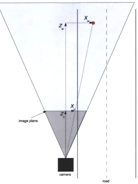
We first define the coordinate system that we will use throughout. Let (Xw, YW, ZW)T be "world coordinates" aligned with the road. The Zw-axis is parallel to the road, the Yw-axis is parallel to the gravity vector, and the Xw-axis is orthogonal to these two (and hence horizontal). Let Zw increase in the direction the camera is aimed, let X, increase to the right when facing in the positive Z. direction and let Yw increase downward. This gives us a right-hand coordinate system.
For convenience we pick the origin of this coordinate system to coincide with the center of projection (COP) of the camera - that way, the road and camera coordinate systems are related just by a rotation, not a rotation and a translation.
Let (Xc,
Yc,
Zc)T be "camera coordinates" with Z, aligned with the optical axis,X, horizontal to the right, and Y vertical down. The origin of this coordinate system is also at the center of projection. These coordinate systems are shown in Figure 4-2.
image plane
x
camera
Figure 4-2: A diagram of the camera and the road showing the camera and world
coordinate systems. The world coordinates X, and Z, of the red dot, as well as the
camera coordinates X, and Zc, are shown. The y coordinates are not shown because
the y-axis is perpendicular to the page, but both Y and Y are increasing downward.
The perspective image projection equations are
x
Xc
f
zc
y
Ye
f
ze
where
f
is the focal length and (x, y) is the position in the image -
measured relative
. ... ... .... - - ." ,
to the image center, or principal point.
Next, the camera is mounted on a tripod that permits two rotations, yaw 0 about
the Y axis, and pitch
#
about the X axis. We then have the relationship between the
world coordinate system and the camera coordinate system
Xj
XW
Y
R
Yw
Ze
ZW
where
1
0
0
cos 0
0 sin0
R =
0
cosq$
sinc
0
1
0
0 -sin 0 cos 0 -sin 0 0 cos 0
or
cos 0
0
sin0
R =
-sin0sin$
cos#
cos0sin#
-sin0cos#
-sin#
cos0cos#
From this we can get the vanishing point (xV, Yv) of the road by projecting the rotated (0, 0, ZW)T to obtain
= tan sec#
= tan#
f
f
These equations allow us to estimate yaw 0 and pitch
#
from the location of the
vanishing point. We can easily find the vanishing point by finding the intersection of
two parallel road lines in the camera image.
Now we can estimate how far a line parallel to Z., such as a road edge or lane
marking, is from the camera. Suppose that the line passes a distance w to the right
of the COP and a distance h below it. This road line projects into a line in the image.
We will estimate the ratio w/h from the angle
of the road line in the image relative
to the y-axis of the image. Then, knowing h we can estimate the horizontal offset w.
Points on the road line have world coordinates
(w,
h,
Z)Tand as Z tends to infinity
the projection of this point tends to the vanishing point. We need only one other point on the projection of this line into the image in order to determine it fully. We find an arbitrary point (xc, yC) in the image. We are only interested in the direction of the line, so we compute
xc - xv XC Xe cos 0 cos 0 - Ze sin0
f Z t Zc cos theta cos
#
and Ye - YV Y Y cos
#
- Ze sin = -- - tan # = f Ze Ze cosq$ where Xc = w cos 0 + Z sin 9Y
= -w sin 9 sin $ + h cos + ± Z cos 0 sin qZe = -w sin 0 cosb - h sin
+
Z cos 0 cos 0We find after some simplification that
Y cos - Ze sin = h
Xc cos 0 cos - Ze sin 9 = w cos q5+ h sin 9 sin
4
consequently
xc - xv wcosq
+
hsin0 sinYC - YV hcos 0
This is the tangent of the angle between the projection of the line and the vertical in the image, so
W Cos
tan =- -
+tan0sin#
h cos
This allows us to calculate w/h from the angle of the projected line and the known camera orientation parameters 9 and
4.
If we know the height h of the COP above the road surface we can then estimate the horizontal offset w of the line from the camera. In our case, we will have a fixed height h as the police vehicle will have aconstant height. If we perform this calculation for two lines, such as lane markings, then we can estimate the distance between them, which would be the lane width.
4.3.2
Software System To Recover Road Lines
Using the machine vision algorithms from the previous section, I designed a software system in C++ to recover road line information given the camera image of the road. The system displays two road lines and a horizon line overlaid on the camera image of the road, which is read using LCM. The officer can adjust these three lines to meet the two edges of the left-most lane and the horizon, respectively. The system uses the intersection of the two road lines to find the vanishing point, and from there calculates the horizontal offset of the road from the camera, as well as the width of the lane. Based on the vanishing point and assuming a flat road, the system can determine the yaw 0 and pitch <$ of the camera relative to the road, and from there determine the entire transformation R from the world coordinate system to the camera coordinate
system. The progression of the system is shown in Figures 4-3 and 4-4.
4.3.3
Position and Velocity Calculation
Once we have calculated the transformation between the camera and road frames, we can track the real world position and velocity of the vehicles using the tracker portion of the software system. First we need to transfer the headlight tracking information from the tracker code to the road lines code just described. This is a little trickier than
simply passing the headlight pixels to the road lines code, as the tracker is working on the short exposure camera, which is a separate camera from the long exposure camera that the road lines code works on. The two cameras are spaced slightly apart, and the timings of the two
cameras are not completely in sync. The timing of the cameras does not really matter for figuring out position information, as the road lines are constant, but the difference in timing can cause a slight offset when displaying tracking information on the road lines image. This problem is hardly noticeable most of the time, but in
Figure 4-3: The road lines program running on a log of the footage from a ride along
with an officer. The user adjusts the road lines shown overlaid on the picture to
fit the lines of the road in the picture. The system then automatically calculates
the distance to the road, the road width, and a transformation from the camera's
coordinate frame to the real world coordinate frame. Based on these calculations, the
system then displays meter markings at increments of 10 meters along the road.
future iterations of the project should be dealt with for increased accuracy.
To take care of the position offset between the two cameras, we calculate a
camera-to-camera transformation using a simple homography, which remains constant,
be-cause the camera rig is constant. We only have to do this once, and can store the
homograph in a config file. Using this simple transformation, we can integrate the
tracker and the road lines code, and then determine position and velocity of tracked
vehicles. To calculate position we simple use the camera-to-world transformation that
we calculated above using the road lines and the vanishing point. We also pass in the
previous frame's headlights from the tracker, which allows us to calculate the velocity
of each tracked headlight pair. In Figure 4-5 we calculate the position and velocity of
Figure 4-4: The user can toggle the level of the road markings between road level
and headlight level. When the road lines are at headlight level, it allows the user to
see whether or not the car corresponding to headlights on the screen is within the
boundary of the road lane. Notice that the car in the left lane has both headlights
between the orange lane lines.
incoming vehicles, and mark any that are in the rightmost lane, closest to the parked
police vehicle.
4.4
Laser Calibration
In addition to the OAM functions performed by the camera, the image from
the
camera is also used by the officer to give the system directions on where to
place
the laser virtual flares. The software system deduces where these flares should
go
based on the camera image of the road, then sends a command to the laser system
for where to fire the laser. This can be tricky, however, because the laser and
the
Figure 4-5: The road lines program after integration with the tracker. The red dots
denote tracked headlight pairs. Blue circles denote vehicles that are in the rightmost
lane, closest to the shoulder.
camera are naturally in different positions, and possibly also different orientations,
upon the police vehicle. Therefore the software system must know the relationship
between the camera coordinate system and the laser coordinate system. In order to
determine this relationship we use the principles of homography.
4.4.1
Homography
We seek to determine the relationship between the camera coordinate system and the
laser coordinate system. The most accurate way to do this is to determine the relative
orientation (translation and rotation) between the laser coordinate system and the
camera coordinate system, using 5 or more pairs of correspondences and a least
squares method[9, 10]. However it was quicker to implement a simple homography,
Camera coordinate system
Y
CLaser coordinate system
Y
x
Czc
Image Plane =(X,,
y,f)
t R
Z
worl
z image Plane=(Xy,,)toR,
Y
wx
W d coordinate systemFigure 4-6: The relationships between the camera, laser, and world coordinate
sys-tems are shown.
f
represents focal length, t represents a translation vector, and R
represents a rotation matrix.
and this doesn't cause a loss of accuracy unless the data is extremely noisy. This
could cause a problem at some point, but for now the homography approach produced
accurate enough results[11, 12, 8]. We can use a homograph because we assume a
flat road, and so we are finding a transformation between two 2-D planes, namely the
image and the road.
In either case, there are some basic calibration parameters we need to determine. Ideally we would want to know where the principal point is, but we use the image center instead, as this is a close approximation for the scale of the road. Image coordinates are in reference to this point, not one corner or another of the image, and in the same units as the focal length.
Many of the projection equations we use are from the chapter on photogrammetry in RobotVision[7]. The camera's perspective projection equations are
xi X! y"
Y
f
ZC,
f
Z,,
where (xi, yi) are the coordinates of the image of the point (Xc, Y, Zc)T measured in the camera coordinate system.
It is important to note that the image coordinates xi and yi are measured relative to the principal point (approximately at the image center) and in the same units, in our case pixels, as those used for
f,
the distance from the center of projection (rear nodal point) to the image plane (approximately the focal length). The principal point is only approximately the image center because of the tangential distortion or imperfect centering of the lens components and other manufacturing defects, in other words the imperfect properties of the camera. We can generally treat the principal point as the image center, as the difference is not enough to effect us on the scale of the road. Similarly the focal length is approximate, as the center of projection can correspond to two nodal points in the imperfect lens. Again, this is not enough to effect us in a noticeable way. Further, the camera coordinates Xc , Y , Ze aremeasured with respect to an origin at the center of projection (front nodal point) with the Z, axis along the optical axis and the Xc and Y axes parallel to the xi and
yi axes in the image plane.
The accuracy with which we can determine the required transformation will de-pend to some extent on the relative arrangement of the camera and the laser. If it were possible to place the center of projection of the camera right at the point of
projection of the laser, then only rotation between them would matter. But of course this is not practical. There may be an advantage to keeping them fairly close together anyway, which we will do, as the final product will be entirely contained in a box on top of the police vehicle.
With the laser, we need to determine the actual angles of deflection of the beam, which will be twice those of the mirror rotations. Next, because rotations do not commute, we need to know in which order the beam from the laser hits the two mirrors. Then the direction of the laser beam can be given as something like
sin 9
cos 0 sin
cos 8 cos q
where 0 and 0 are the deflection angles of the two mirrors. This expression will look slightly different, depending on the arrangement of mirrors and choice of coordinate axes, which we will examine in the following section.
There is an additional issue with the laser in that the mirrors rotate about axes that do not intersect. This makes the calculation of the exiting beam much harder, but we can ignore this based on the large ratio between the distance to the road surface (many meters) and the distance between the two mirror axes (< 10 mm).
The transformation between any arbitrary world coordinate system X", Y", and
Z, (not necessarily corresponding to the world coordinate system from the previous section) and the camera coordinate system is given by a rotation and a translation
Xc XW
Yc =R Y) +t
where R is an orthonormal rotation matrix and t = (X , Y0 0, ZO)T, is the translational offset.
world coordinate system in such a way that Zw, = 0 for points on that surface. Then
Xc = rnlXw + r12Yw + XO
Y= r2 1Xw + r22Yw + Yo
Ze = r31Xw + r3 2Yw + ZO
where rij are the components of the rotation matrix for row i and column j. We can also write this as
XC
YC
Ze)
rin r1 2 Xo r2 1 r22 YO r3 1 r2 2 ZOXW
Yw
1J
Using the perspective projection equation we see that
wi Xc k yi Y f Ze where k = (Ze/f). So xi
r,
k y r21 f r3 or kf xi yiI 1 or=I
frn
f r21 r12 X0 r2 2 Y r22 ZO)
fr 12 f X0 fr22 fY r2 2 Zoki
ki y Me XWYW
yw XwYW
XW
YW
C
)
That is, there is a simple linear relationship between homogeneous coordinates on the world plane, in our case the road surface, and homogeneous coordinates in the image plane.
We can think of the laser as something like a reverse camera, that fires rays of light from its COP rather than receiving rays of light like the camera. We can imagine a plane a distance f in front of the device and specify the directions of rays from it
by coordinates x, and y, where the ray intersects this plane. Then there is a similar
relationship between coordinates in this plane and world coordinates on the road, just
X1 XW
k, y, =AM YW
We can combine these two transformations to find a transformation between laser coordinates and image coordinates:
Xi X1
k
yi
= My,
where M = M1M;j.
The calibration task is that of finding M, a 3 x 3 matrix, using correspondences between laser coordinates (xi, yi) and image coordinates (xi, yi). The matrix M has
9 elements, but since it relates homogeneous coordinates, its magnitude does not
matter. So we have only 8 unknowns - we can fix one component, say M3 3 = 1, and
solve for the rest. We now have
kxi
= M1. (XI, yI, 1)Tkyj = M2. (X1, yI, I)T
where M1, M2 and M3 are the three rows of the matrix M and the dot denotes dot
product. Using the last equation to substitute for k in the first two equations we obtain
m1 1X1
+
m12yI + Mi1 3 - m31xix - m3 2xiyl - m33Xi = 0 m2 1x1 + m 2 2y1 + m23 - m3 yxi1 - m3 2yi - m33Yi = 0We obtain two such linear (homogeneous) equations in the unknown elements of the matrix M for every correspondence between a laser direction (xl, yl) and the coordinates of the image (Xi, yi) of the spot that the laser makes on the surface. If we collect enough correspondences, and add the non-homogeneous equation n33 = 1, we can solve the resulting set of linear equations for the components of the transformation matrix M. Because there are 8 unknowns, we need 4 correspondences to produce 8 linear equations, which we can just solve using Gaussian elimination.
Once we have the transformation matrix M, we can then convert any image point (Xi, yi) to a laser point (xi, yj). The laser, however, does not understand this coordinate system, and only takes mirror angles as input. Therefore we must find a transformation between the laser points (xi, yi) and the command angles to send to the laser. To figure out this transformation, we will examine the galvanometers of the laser in greater detail.
4.4.2
Galvanometers
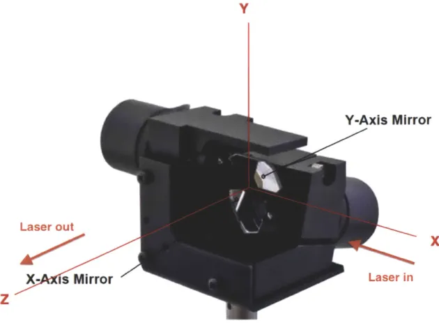
The laser contains two galvanometer-driven mirrors, which control the direction of the laser beam. First, let's define the coordinate system for the galvanometers.
Let Z be the direction of the beam out of the mirror system at zero deflection (i.e. perpendicular to the plate with the three screws visible in Figure 4-7). Let X be the direction opposite to that of the laser beam where it comes into the mirror system (i.e. parallel to the line between the bottom two screws on the front plate in the figure). Let Y be upward, perpendicular to the X- and Z-axis (i.e. parallel to the line connecting the two left screws in Figure 4-7). These axes form a right-hand
Y
Y-Axis
Mirror
Laser out
X-
is Mirror
Z
Ls i
X
Laser in
Figure 4-7: The coordinate system for the galvanometers.
coordinate system.
Next, we define the positive angle of rotation of the galvanometers as clockwise
when viewed from a point along the axis on the mirror side of the motor. The
deflection of a beam by a mirror can be described by
=Out
=
in-
2(in *
n)n
where
jn is a unit vector in the direction of the incident beam and bOut is a unit
vector in the direction of the reflected beam and
fiis the unit normal to the mirror.
We can verify that the emitted angle equals the incident angle, and that the three
vectors bin, bout, and ii are coplanar using
bin - bout = 2(bi - )n (bin + bout) -
n
= 0(-bin) - = bout
-[bin bout i] = (bin x bout) -i = 0
Next, we consider the orientation of the two mirrors. The axis of rotation of the second, "Y-axis" mirror is k = (1, 0, 0)T . The normal to this mirror is
f2 = (0, c2, S2)'
where c2 = cos (02 + 020), S2 = sin (02 + 020), with 02 being the rotation of the axis of
that galvanometer from its rest position and 020 being the rest position angle
(~
r/4).The axis of rotation of the first, "X-axis" mirror is (0, se, c,)T where ce = cos E, s, = sin f and E is the angle of inclination of the galvanometer axis with respect to the horizontal plane. Measurement of the drawing from the manual of the galvanometers indicates that ce~ 11.5[201. The normal to the first mirror is
li = (si, cicE, -cise) T
where c = cos (01
+
01o) and s, = sin (01+
010), with 01 being the rotation of theaxis of that galvanometer from its rest position and 010 being the rest position angle (wr/4).
The beam initially enters the assembly traveling in the negative X-direction
bo
= -R = (-1, 0, O)Tafter some simplification,
C1
bi =
S
1c,SSisF
where C1 = cos (2(01 + 010)), and S1 = sin (2(01
+
01o)) (note upper case C1 and S,now for trigonometric functions of double angles).
After reflection by the second mirror the beam direction is b2 = - 2( 1 -
n2)2
or, after some simplification,
C1 2 = S1(-C2C: + S2s)
S1 (C28,5 - S2Ce)
where C2 = cos (2(92 + 920)), and S2 = sin (2(92 + 020)) (note upper case C2 and S2 now for trigonometric functions of double angles). This can also be written as
C1 b2 = -S1C2
S1SA
where C2 = cos (2(02 + 020) - E) and S2 = sin (2(92 + 920) - E). Note how we can compensate for the angular offset of the axis of the first galvanometer by adjusting the at-rest position of the second axis so that the exit beam travels parallel to the Z-axis when the galvanometers are in their rest position. All we need to do is set
020 = E/2.
Finally, if O1o = 7r/4, then Si = cos (201) and C1 = - sin (201). So we end up with
- sin (291)
2 =cos (s6i) sin (292)
cos (sO1) cos (292)
sign on the X-component which in practice is taken care of by considering counter-clockwise rotation of galvanometer 1 as positive. Also, note the double angles due to the fact that reflection of light doubles the angles. The rotation commands to the galvanometers already take this into account and correspond to 20, and 202.
Projecting the exit beam onto a planar surface perpendicular to the Z-axis at distance
f,
which corresponds to a laser point (Xi, yi), we obtainX
- tan(201)
sec (202)Y1 =
f
tan (202)for the position of the spot. Note that the y-position is affected only by 02, while the x1-position depends on both 02 and 01. The sec(202) multiplier stretches the
x1-component when 02 is non-zero.
Conversely, we can get the galvanometer commanded angles from desired positions in the plane using
-201 = arctan
(2
Vf2 +yJ2
202= arctan
(j)
This provides the galvanometer command angles given a desired position in the pro-jection plane. We can use these formulas to determine the command angles to send
to the laser to fire the beam in a desired direction (Xi, yi).
4.4.3
Calibration Software System
I designed a calibration process, and added it to the road lines software system. The
procedure consists of a series of steps performed by the user of the software system, which will most likely be the officer. The officer follows instructions on the screen, and the software system runs the algorithms described in the previous sections to determine a transformation M between the camera and laser coordinate systems. The
software communicates with the laser using LCM, sending it galvanometer command
angles.
Generally the camera and the laser coordinate systems are close together and
pointed in generally the same direction, although this procedure works for any
ar-rangement of the laser and camera. The system has no knowledge of the laser's
orientation, and only can see through the camera coordinate system. The system
initially assumes an identity transformation between the two coordinate systems,
al-though this is never actually the case, as even if the camera were right on top of the
laser and pointed in the exact same direction, there is some scale factor that differs in
the two coordinate systems. By the end of the calibration process the system knows
M and can draw any arbitrary series of laser points in the real world based on the
user's clicks on the camera image.
The steps of the calibration process are as follows:
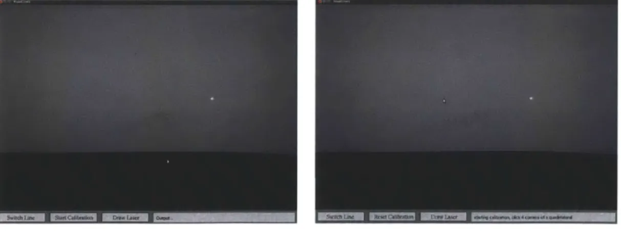
1. First the user clicks on the 'Start Calibration' button in the menu bar.
Direc-tions are displayed in the output section of the menu, which tells the user to
click in a quadrilateral on the road surface to send to the laser.
(a) User clicks on 'Start Calibration'. (b) The system prompts the user to click four corners of a quadrilateral.
Figure 4-8: Step 1.
2. The user clicks on the four corners of a quadrilateral. The system calculates the
corresponding galvanometer command angles, based on its current idea of the
transformation M, which is initially just the identity. The laser points
corre-sponding to the clicked corners then appear on the world surface. Additionally
a plot of the galvanometer command angles appears, as well as a graph of the
clicked points in the laser coordinate system.
Figure 4-9: Step 2. The user clicks a quadrilateral (light blue), which the system
transforms to a series of laser points, as seen to the upper right of the clicks. A plot
of the galvanometer command angles appears in the top left of the screen, and shows
the angles of the two motors, with a green dot that follows the angles being sent by
the software to the laser. In the top right of the screen a plot of the clicks in the laser
coordinate frame appears, with points in blue.
3. The user is prompted to click on the four laser points as they appear on the
screen, in the order corresponding to the order clicked. With each clicked laser
point, the system gets a laser-camera correspondence, as described in the section
on homography. Once the system has four such correspondences, it can perform
the algorithms previously described to calculate the transformation matrix M.
After these four clicks, the system should be fully calibrated. If the calibration
is a little off, then the user can reset the calibration process and start over.
Figure 4-10: Step 3. The user clicks on the laser points corresponding to the corners
of the quadrilateral. These clicks appear in green. Notice the blue points in the laser
frame have changed position, as the transformation matrix M has been updated, and
so the laser frame coordinates of the calibration quadrilateral have shifted.
4. The user can now click on the 'Draw Laser' button to command the laser to
draw out any arbitrary shape. The user clicks on an arbitrary series of points on
the world surface in the image, and the system stores an array of galvanometer
command angles corresponding to these image points.
5. When the user clicks on the 'Send Laser' button, the array of galvanometer
command angles is sent to the laser, and the laser outputs the desired points
on the world surface.
Figure 4-11: Step 4. The user clicks the 'Draw Laser' button, and clicks a series of
points in a pattern on the world surface. Notice the order of the points clicked.
This procedure allows the user to easily calibrate the camera and laser coordinate
systems. A demonstration of the procedure in action is shown in Figure 4-13. This
should only need to be done once for the final product, but depending on how static
all of the parts are, can be done occasionally and very quickly to keep the two systems
calibrated. The laser drawing functionality will allow the officer to design a pattern
of virtual flares on the road surface with a simple series of clicks, saving him or her
time and energy on placing real flares on the road.
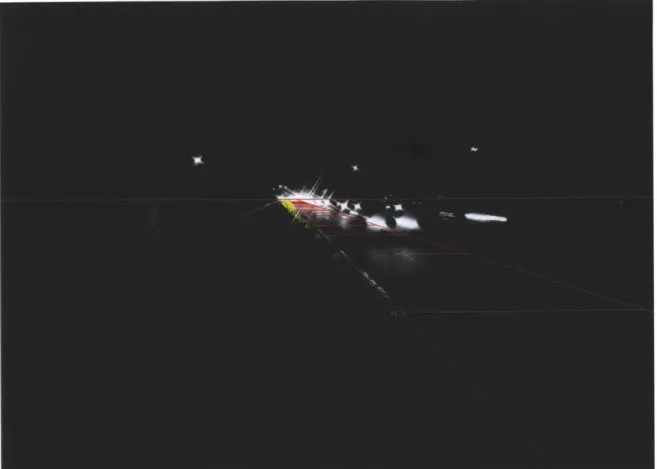
Figure 4-12: Step 5. The user clicks the 'Send Laser' button, and the galvanometer
command angles corresponding to the pattern are sent to the laser. Notice the star
pattern. The laser in its current state moves between laser points slower than the
final laser will, and some intermittent laser points are produced in between each point.
Also notice the curve of the lines between each laser point. This is due to the angular
nature of the galvanometers, and so the shortest path between two mirror positions
does not necessarily translate to the shortest path on the world surface. Finally note
that this example of the system uses a flat vertical wall, instead of a horizontal road.
This should not make any difference, as the system only assumes a flat surface, and
the code has been run on a horizontal surface and works just as well.
(a) A user running the calibration procedure on a laptop.
(b) The lasers projected on a wall.
(c) The laser system. The laser source is on the right, and the laser travels through a series of optical lenses in the middle, then enters the galvanometers on the left and is projected out of the hole on the left facing forward.