HAL Id: hal-02046608
https://hal.archives-ouvertes.fr/hal-02046608
Submitted on 22 Mar 2021
HAL is a multi-disciplinary open access
archive for the deposit and dissemination of
sci-entific research documents, whether they are
pub-lished or not. The documents may come from
teaching and research institutions in France or
abroad, or from public or private research centers.
L’archive ouverte pluridisciplinaire HAL, est
destinée au dépôt et à la diffusion de documents
scientifiques de niveau recherche, publiés ou non,
émanant des établissements d’enseignement et de
recherche français ou étrangers, des laboratoires
publics ou privés.
Mantle dynamics with induced plate tectonics
Y. Ricard, C. Vigny
To cite this version:
Y. Ricard, C. Vigny. Mantle dynamics with induced plate tectonics. Journal of Geophysical Research,
American Geophysical Union, 1989, 94 (B12), pp.17,543-17,559. �hal-02046608�
JOURNAL OF GEOPHYSICAL RESEARCH, VOL. 94, NO. B12, PAGES 17,543-17,559, DECEMBER 10, 1989
MANTLE DYNAMICS WITH INDUCED PLATE TECTONICS
Yanick Ricard and Christophe Vigny
D•partement de G•ologie, Ecole Normale Sup•rieure, Paris
Abstract. Mantle circulation and plate tecto- nics can be described by means of two scalar fields. The poloidal field is related to horizon- tal divergence, i.e., to the vertical mass flux. The toroidal field expresses the shear deforma- tion or the rotations within spherical shells. For the Earth, the surface kinetic energy is known to be equally distributed between the two fields. In recent years the lateral mantle den- sity variations revealed by seismic tomography have been introduced in dynamic mantle models which have predicted the major features of both the geoid and the surface divergence. These models assumed a spherical symmetry of the theo- logical properties of the Earth. However, with this assumption, the Navier-Stokes equation im- plies that mass heterogeneities cannot drive any toroidal motion. This prompted us to develop a new model which takes into account the existence of rigid and independent plates. These plates break the spherical symmetry assumed in all earlier models. They modify the mantle circula- tion and hence the predicted surface observables such as displacement and gravity. In this paper, we first explain by means of a very simple two- plate model, how the poloidal flow caused by mantle heterogeneities can be converted to sur- face toroidal motion. We then apply the model to the real Earth with its major plates and compare our predictions to those deduced from a more classical Earth model having a uniform free slip condition at the surface. Taking the seismic to- mography pattern as a picture of the mantle mass heterogeneities, we achieve a highly satisfactory fit to the observed plate velocities. This new theoretical framework also improves the geoid prediction.
Introduction
In the last few years, the complex relation- ships between deep mass heterogeneities and sur- face observables, such as topography, horizontal surface velocities, and gravity, have been deri- ved by various authors [Kaula, 1975; Hager and 0'Connell, 1979; Ricard et al., 1984; Richards and Hager, 1985; Forte and Peltier, 1987]. In most of these studies the real Earth is modelled as a self-gravitational viscous sphere. The vis- cosity is assumed to be Newtonian and only varies with depth. The lateral density variations within the mantle induce a flow which deflects the various interfaces such as the Earth's surface and the core-mantle boundary. The gravity field depends both on the internal masses and on the shapes of the dynamically perturbed interfaces.
The predictions of these models have been test against observations. Using a realistic mass dis- tribution for slabs and assuming that seismic to- mography reflects the deep mantle structure, sa- tisfactory geoid configuration and surface velo- city divergence have been computed [Hager et al., 1985; Forte and Peltier, 1987; Ricard et al., 1988].
The physical equations which have been widely used to model the large-scale dynamic behavior of the Earth are the Navier-Stokes, Poisson, and mass conservation equations which read
• V V = Up - p VU - 6p g (1) V 2 U = - 4 =G6p (2)
vv= o (3)
In these expressions, the velocity field V is induced by the nonhydrostatic pressure p and by the lateral density variations 6p. The perturbed gravity potential U due to the density variations 6p appears in equation (1) describing the dynamic behaviour because of the self-gravitational ef- fect. The viscosity • and the density p are as- sumed to be uniform, and G is the gravitational
constant. By inspection of equation (3), one sees
that the velocity V is the curl of a vector field and can be written in the most general way on the form:
V = V © Te• + V © V © Se•
(4)The scalar functions S and T are the pol•idal and
toroidal
components
of the flow, and e• is the
unit radial vector. The physical meaning of thesenew fields is easily understood. •t can be shown
that the horizontal divergence V H V, which is the
divergenc•
of
the horizontal
component of the
velocity V is related only to the poloi•al •omp9-
nent,
whereas the radial vorticity
( V © V ) e•
depends only upon the toroidal component. The re- lationships between these fields readr 2 Or
H
( V© V ) e• = -V H
(6) 2 is the horizontal Laplace operator Atwhere V H
.
the Earth's surface, the converging zones of sub- duction or collision and the diverging ridges ex- press the existence of internal poloidal flow. On the other hand, the strike-slip zones reveal the vigor of the toroidal component. Taking the curl
Copyright 1989 by the American Geophysical Union. of the Navier-Stokes equation (1) and expressing
V as a function of S and T following equation
Paper number 89JB01292. (4), one can derive two new equations which de- 0148-0227/89/89JB-01292505.00 couple the poloidal and toroidal fields by
17,544 Ricard and Vigny: Mantle Dynamics With Induced Plate Tectonics
gp g generates surface observables which contains
V q S =
(7)
other wavelengths.
These models
with long-wave-
•
length viscosity variations excite radial vorti-
V 2 T = 0
(8)
city
[Ricard et al.,
1988], but the toroidal en-
ergy remains rather low in comparison with theThus the internal mass heterogeneities induce the poloidal energy. The energy equipartition between poloidal field, but there are no excitation toroidal and poloidal fields seems to indicate sources for the toroidal field. The latter should that viscosity variations occur on a length scale therefore vanish. For the real Earth, this is not smaller than the characteristic plate size. For the case. On the contrary, a quasi-equipartition the real Earth, the sharpest viscosity contrasts of kinetic energy between the two modes is obser- occur, of course, near plate boundaries. In what ved. For whole mantle problems, the global scale follows, we present a model which takes the very of the fields make the spectral representation in existence of plates into account. This model term of spherical harmonics appropriate. The explains the generation of the toroidal flow and power spectra of both the observed poloidal and clearly demonstrates that surface plates strongly
toroidal
surface fields vary like Z -2 [Hager and
affect the whole mantle dynamics.
0'Connell, 1979; Forte and Peltier, 1987]. This striking observation obviously means that the theoretical framework given by equations (1),
(2), and (3} is insufficient. The Physical Model
The only way to generate toroidal motion in a
viscous fluid is to allow the viscosity to vary Our model consists of a spherical self-gravi- laterally. In this case the Navier-stokes equa- tational viscous mantle overlaid by rigid plates
tion (1) is not valid and must be replaced by the
and surrounding an inviscid core. The number and
more general momentum
equation (9) which reads
the shape of plates represent a priori data. In
other words, we do not deal with the problem of
• 2 •
• V
V + 2 • 9 • = 9 p - p 9 U - 6p •
(9)
their creation or evolution. Deep mantle hetero-
geneities produce a circulation which drives the
Here • is the strain rate tensor, and • is the
overlaying plates. There are no direct interac-
viscosity
which can vary spatially
within the
tions
between plates,
but the motion of a given
fluid. plate partly controls the mantle flow and therbyFor simplicity
let
us neglect the Earth's
indirectly
interacts with the others. Mechanical
sphericity and assume
that the gravity g is par-
equilibrium requests
that the torque of all ap-
allel to the vertical unit vector z. To infer the plied forces on each plate be zero [Lliboutry,
generation of toroidal motion, let us again take
1972; Forsyth and Uyeda, 1975]. Our mathematical
the curl of equation (9) and project the resul-
approach consists
in
superposing two subsolu-
ting
equation onto the vertical vector. After a
tions. The first one is excited by imposed inter-
somewhat cumbersome algebra, one finds nal loads with a no-slip condition at the outerspherical surface. The second one has no internal
1 •
M V 2[ + • [ • M = _ _ ( • M © • p ) z (10)
loading and is excited by a horizontal
surface
• velocity field described by an unknown set of rotation vectors. The values of these rotation
where [ = ( 9 © • ) • is the vertical vorticity.
vectors are deduced from the balance of the
This last equation was given incorrectly in a pa- mechanical torques applied on each plate by the per by Kaula [1980] where it appeared without the two subsolutions. For mathematical convenience
term on the right hand-side. It is complex, but
the computation has been done using a generalized
its
physical meaning is clear. To drive the to-
spherical
harmonic representation
truncated for
roidal field, the Earth's dynastic
be•avior, thus
degrees
larger than 15. This formalism
was intro-
needs to produce a nonzero ( V • © V p ) z. In
duced in seismological
theory [Phinney and
other words, lateral
pressure variations must
Burridge,
1973] and can readily be applied to
include
a component orthogonal to lateral varia-
dynamical problems. It
enables one to handle
tions in viscosity.
This also indicates that
simultaneously scalar, vectorial,
and tensorial
radial
viscosity variations are inefficient in
quantities,
and it
provides an elegant way of
exciting
toroidal motions. These conclusions
writing differential
operators like gradient,
remain true for a spherical Earth, but other com-
divergence, or curl.
The indices n, Z, and m
ponents related to [ and its partial derivatives
refer
to a representation on the basis of gener-
appear in equation (10). The steeper the visco-
alized
spherical harmonics. In the mathematical
sity
transitions, the more vigorous the toroidal
appendix, the relationship between the components
v n*m of the surface velocity field and the hot-
motion.
Long-wavelength
viscosity
variations
are known izontal shear
stress components
v nzm
intgenerated
by
to exist within the Earth. Some of them correlate internal loads with a no-slip boundary condition
with tectonic provinces like young oceans and old
at the surface is found to read (see equation
cratons. Their effects on global dynamic
models
(A18})
have already been analyzed
[Ricard et al., 1988].
R
-
More generally lateral variations
'in viscosity
v nz• --G' ( G K G' ) 1G v n'z'•'
= int(11}
within the deep convecting mantle can be related •0 to temperature and thus be associated with den-
sity
variations
[Richards et al.,
1989]. The
Here R is
the Earth's radius, and •0 is the re-
general conclusion of the two papers just quoted ference viscosity. The matrix K describes the is that a mass anomaly with a given wavelength linear relationship between imposed surface velo-Ricard and Vigny: Mantle Dynamics With Induced Plate Tectonics 17,545 1 .I I ! I I i f I I 15.88 18.88 5.88 8.80
•
-5.8•)
- 5.•)0
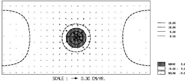
"':::"':'""• BELOI• -5.00 SCALE ' --• 8.38 CM/YR.Fig. 1. Computed geoid and surface velocity fields induced by a circular mantle mass anomaly located at a depth of 300 km and having the shape of a spherical cap of radius 1500 km. The model Earth is mapped through a linear representation of both longitude and latitude. Its interior has a purely spherical symmetry and is made up of three layers: a lithosphere with viscosity 1022 Pa s, an upper mantle with viscosity
102• Pa s , and a stiffer
lower mantle with viscosity 1023 Pa s. The computation was
carried out up to the harmonic degree • = 15. The level lines for the geoid are 5 m apart and the regions above 5 m are shaded. The surface velocity field radially con- verges toward the center of the anomaly and reaches a maximum of 0.3 cm/yr.they generate in the absence of internal loads wavelength of the internal load, it produces a
(see (A8)) velocity field containing all possible wave-
lengths. Nevertheless, numerical experiments have •0
V nZ• = -- K V
n' Z'•'
(12)
ext R
shown that the long-wavelength results are quite insensitive to the short-wavelength components of the loads.
The operator G expresses the coupling between the induced plate kinematics and the internal cir-
culation. In the absence of rigid surface plates,
A Numerical Example
G equals the identity matrix, and (11) readssimply
To get some insight into
the physics of our
R
problem, let us take a very simple Earth model
V
nZ• = --K -1T n'Z'•'
int(13)
where the mantle is overlaid by two hemispheric
•0 shells of thicknesses L = 100 km. The mantle flow is driven by a circular, horizontal mass hetero- The general formalism which enables one to com- geneity of radius R = 1500 km at a depth z =300
pure K and T nzm
int'
was fully described in recent
km. This load is located
just below the great
papers [e.g.,
Ricard et al.,
1984]. It consists
circle
defining
the boundary between the two
in computing Green's excitation functions for plates. It has a prescribed surface density ofeach spherical harmonic degree. A radial convo-
106 kg/m
2 , and therefore would correspond, as-
lution of the Green's functions with the radial suming isostasy, to a surface topography of 350 load distributions is then carried out for every m. The upper mantle viscosity is fixed at degree g and order m. The details for construct- 102• Pa s, whereas three different viscosities,
ing the matrix
G are found in the mathematical
amounting to 102• , 1022 , and 1023 Pa s, are con-
appendix. sidered for the lower mantle. The results of ourOur numerical code thus computes the pole and models are compared to those produced by classi- the rotation velocity of each plate caused by the cal models with a uniform free slip condition at internal load distribution within the mantle. the surface. Both types of models, with and Such a velocity pattern contains both poloidal without plates, have the same internal viscosity and toroidal components. This is due to the im- profile except for the presence of a 100-km-thick
posed rigidity of plates which only allow defor-
lithosphere with viscosity 1022 Pa s in the first
mation near their boundaries. The generation of case.
toroidal motion is the major novelty of this pa- First, we consider a model Earth with a uni- per. The global dynamics is drastically different form free slip condition at the surface and with from that of earlier Earth models with free slip a viscosity increase by a factor 100, 10, or 1 at or no-slip condition on the outer surface. The 650 km depth. Figure 1 depicts the surface velo- predicted topography and geoid will of course be city field and the induced geoid for a viscosity affected by the presence oP plates. In this new ratio of 100. The dense mass sinks within the framework one should notice that whatever the mantle and induces a symmetrically converging
17,546 Ricard and Vigny: Mantle Dynamics With Induced Plate Tectonics 1.0 0.5 0.0 -0.5 -1.8 i i i i l 0 80 120 180 2qO 300 LONGITUOE 360 -18 0 80 120 180 LONGITUDE i I 240 300 360
Fig. 2. Equatorial profiles of the geoid and the velocity. The solid curve corresponds to the sec- tion of Figure 1 where the viscosity of the lower mantle is 100 times that of the upper mantle. Two other computations for a viscosity jump reduced to a factor of 10 and for a uniform mantle led to the dashed and dotted profiles, respectively. For a model Earth with a purely radial viscosity and our chosen circular mass anomaly, the sections are the same across all great circles crossing the center of this mass.
purely poloidal flow. The geoid exhibits a maxi- mum located just above the deep heterogeneity which has the same symmetry as the load. Equato- rial profiles of the velocity and the geoid are displayed in Figure 2 (top and bottom). The solid curves correspond to the equatorial section of the map depicted on Figure 1. The dashed curves stand for a viscosity jump by a factor 10 at 650
km, and the dotted curves correspond to a uniform
mantle. The velocities (Figure 2, top) are anti- symmetrical and reach their extrema above the edge of the deep mass. The undulations are only due to Gibbs' effect related to our truncation degree Z = 15. The maximum velocity value in- creases as the lower mantle viscosity decreases,
and it reaches 0.9 cm/yr for a uniform mantle. The sign of the induced geoid (bottom) changes
according to the value of the viscosity jump at the upper-lower mantle interface. This result is
well known [Ricard et al., 1984; Hager, 1984; Lago and Rabinowicz, 1984]. Indeed, in a mantle with uniform viscosity, the dense mass deflects the lithosphere downward by 332 m, somewhat less than for isostasy. Nevertheless, this surface mass deficiency yields a larger geoid signal than the deep source, and the resulting geoid is a low of 14 m amplitude. A stiffer lower mantle sup- ports the internal load more efficiently, so that
the induced surface topography is smaller and yields a weaker contribution to the total geoid signal. For example, for a viscosity jump of 10, respectively 100, at 650 km depth, the surface depression reduces to 273 m, respectively 167 m. The total geoid is still a low of amplitude 3 m in the first case. It becomes a high of 17 m in the second case.
Second, we consider the same Earth structures but introduce two hemispheric plates. The results are indeed very different. The induced geoid and plate velocities are given in Figure 3 for a mantle viscosity contrast of 100. The convergence is now perpendicular to the ridges and has thus
-,.- --• • -,.-,:..•..'.':.:.?
••,-•.:•.':.:•?:,:..•.
•'-
...
'
:
...
"
:::::::::::::::::::::::::::::::: r ::::::::::::::::::::::::::::::::i::::!:,•i::i::f-•--•
• -'"'
' '•
...
::::::::::::::::::::::
ß ---,a.•,
:::::::::::::::::::::::::::::::::
-
• •.- -•-
_ ...
..,_
..,_ ,,.._
4 3 2.88 1 8 .B8 ... -1.88 ... -2•
-1.88
- 1.08
'x:' '•.,•..::• BELOW -1.88 SCALE : • 0.06 CM/YR.Fig. 3. Computed geoid and velocity fields induced by a circular mantle mass anomaly of radius 1500 km located 300 km below the border of two hemispheric shells. This bor- der runs through the middle of the map from north to south. This figure should be com- pared with Figure 1. The level lines for the geoid are 1 m apart and the regions above 1 m, respectively below -1 m, are shaded in dark, respectively in light. The plate mo- tions correspond to two opposite rotations around the polar axes with an equatorial velocity of 0.06 cm/yr.
Ricard and Vigny: Mantle Dynamics With Induced Plate Tectonics 17,547
lost the symmetry of the load. The velocity is is 4 times lower than that obtained for a free maximum at the equator and vanishes at the poles. slip model. This is because the plate, driven by The geoid is more complex than the one depicted the mantle flow near the load, has to drag the in Figure 1. It superimposes a new effect related underlying mantle over most of the Earth's sur- to the induced plate tectonics on the gravity face. In this simple example, the shape of the signal linked to the deep mass. An overpressure velocity pattern is independent of the viscosity exists underneath the converging zones and a profile which only imposes the overall amplitude. pressure deficit below the diverging zones. This The induced topography is made of a long-wave- horizontal pressure gradient drives the return length component determined by the plate geometry flow which now has a geometry imposed by the and a local component just above the load. The plate configuration. It generates an additional resulting geoid shows these two contributions and geoid high over trenches and a geoid low over again changes sign above the internal load when ridges [Schubert et at., 1978; Ricard et at., the viscosity ratio between upper and lower 1984]. In Figure 3, the surface velocities and mantle varies from 1 to 100. The more the visco- the geoid are symmetrical with respect to the sity stratification confines the return flow, the great circle following the plate boundary. This more the computed geoids with and without plates is, of course, related to the particular location differ.
of the mass, just beneath this circle. The same Let us now turn to the problem of the energy mass, located below the center of one of the distribution between the poloidal and toroidal hemispheric shells, would generate no surface motions. Figure 5 depicts the power spectra of motion and the same geoid signature as if a no- the two components as a function of Z. On top is slip condition was applied. Figure 4 displays the plotted the curve corresponding to the power horizontal velocity and the geoid along the equa- spectrum of the velocity field for the Earth tot, for the three chosen viscosity stratifica- model without plate given in Figure 1. This graph tions. The velocity is quite uniform on each reminds us that no toroidal field can be genera- plate, and it increases again as the lower mantle ted in this kind of model. The increase for viscosity decreases. The absolute value of 0.25 degrees 13-15 is due to side lobes in the power cm/yr is reached for a uniform mantle. This value spectrum linked with the geometry of the deep
1.0 -1.0 0 I I I I 120 180 2'qO 300 360 LONGITUDE 20 10 i.-q r
o
•
/
• -10 \ /: ß -20 I I ', i i 8 60 128 188 248 300 368 LONGITUOEmass heterogeneity. The bottom curves are for an Earth model with plates and are associated with the velocity field depicted in Figure 3. The sym- metries of the pattern requires poloidal, respec- tively toroidal, components of even, respectively odd degrees Z to be zero. Even for this very simple example a comparable energy is found in the two modes. The power spectrum of the polo- idal, respectively toroidal, surface field varies
as 0.02 Z
-•'8
,respectively 0 06 F 2'9 The rota-
ß ,tion of two hemispheric shells toward each other creates a strong vorticity in the vicinity of the two poles.
Does the existence of plates necessarily leads to an equipartition of kinetic energy between poloidal and toroidal components of the velocity field? In the case of two hemispheric plates with rotation poles located at the center of each plate, one would have a situation where only the toroidal field is present. However, this sort of hemispheric twist cannot be excited by internal loads. For a given plate configuration, the dis- tribution of energy is certainly sensitive to the configuration of the rotational poles. In the simple case discussed above, any internal load distribution will locate the rotational axes on the plate boundary and lead to equipartion be- tween the two velocity components at the surface.
Application to the Real Earth
In the previous section, we described the Fig. q. Equatorial profiles of the geoid and the basic physics of global mantle circulation with velocity for a model Earth with two hemispheric induced plate tectonics. In what follows, let us shells. The solid, dashed, and dotted curves cot- apply our code to a realistic Earth model. To run respond to a lower mantle viscosity 100, 10, and our program, we need three different data sets: 1 times that of the upper mantle, respectively. first, the number and the shapes of plates which The upper mantle viscosity remains equal to define the coupling between the surface and the
102• Pa s.
This figure
should be compared with
mantle;
second, the three-dimensional distribu-
Figure 2, where the profiles, drawn at the same tion of internal masses which drive the flow; and scale, were obtained for a model Earth without third, the mechanical structure of the Earth plates. characterized by viscosity and density profiles.17,548 Ricard and Vigny: Mantle Dynamics With Induced Plate Tectonics 1E-el '-,. 1E-½2- c) LLI z 1E-•3 - H LLI m 1E-04 - 1E-El5 WITHOUT PLRTES
F] poloidal
m BEGREE 1 1E-El1 '-,. 1E-82 - c) LLI z 1E-133 - LtJ m 1E-84- 1E-½5 NITH PLRTESFq poloidal
(D tonoidal DEGREE 1Fig. 5.
Power spectra of the velocity fields depicted in Figure 1 (top) and Figure 3
(bottom). The upper graph corresponds to a model Earth with a uniform lithosphere.
This assumption imposes a zero toroidal field.
A lithosphere broken into two plates
excites a toroidal field as seen on the lower graph. In this case, the kinematic en- ergies of both the toroidal (circles) and poloidal (squares) motions are somewhatcomparable.
We have chosen to take 1! main plates into ac-
fined by their
seismicity
[Hager, 1984]. The
count: African, American, Antartic, Arabian, downgoing slabs are assumed to have a surface Caribean, Cocos, Eurasian, Indian, Nazca, Paci- density of 107 kg/m:. This last value can be de- fic, and Philippine. In the lower mantle, the duced from a seafloor bathymetry increase of 4000 mass heterogeneities are supposed to be propor- m between young and old oceans. Other choices of tional to the seismic velocity anomalies revealed this three scaling factors could have been madeby
tomography [Dziewonski,
1984].
A scaling
and will be discussed later. The various compo-
factor 0v./0p = 6 km s-•/g cm
-3 has been chosen.
nents of our mass heterogeneities are expressed
This valu• is in the range of experimental in spherical harmonics
truncated
beyond
Z = 6 for
measurements for
oxides [Sumino and Anderson,
the lower mantle, beyond Z = 8 for the upper
1984] and roughly corresponds
to what has been
mantle, and beyond Z = 15 for the slabs. The
proposed on the basis of
spherically
symmetric
radial
properties of our model Earth are charac-
models fitting the observed geoid [Hager et al.,
terized by a density profile according to the
1985; Ricard et al., 1989]. For the upper mantle
Preliminary
Reference Earth Model (PREM)
we add two different data sets describing mass
[Dziewonski and Anderson, 1981] and a viscosity
heterogeneities.
The first
one is proportional to
increase by a factor 50 at 650 km. A reference
upper mantle seismic tomography [Woodhouse
and
value
for the viscosity is
chosen afterward to
Dziewonski,
1984] with
a conversion factor
match the amplitudes of the predicted surface ve-
0vs/•p = 30 km s-•/g cm
-3. This high value tends
locity field to the observed one.
to damp the contributions of seismic heterogene-
For comparison we carried out two computations
ities
which may, in
part, have a petrological
with
the same mass heterogeneities but different
rather
than thermal origin. The second one de-
lithospheric
layers.
In the first,
the litho-
Ricard and Vigny: Mantle Dynamics With Induced Plate Tectonics 17,549
100 times that of the upper mantle. In the sec- Figure 7 depicts the same correlation curves, ond, we break the lithosphere into 11 rigid but for the model Earth with 11 plates. In compa-
plates.
In
both cases,
we compute the global
rison
to Figure
6 there is a great improvement.
dynamic response of our model Earth and, particu- Both poloidal and toroidal velocity components larly, the three surface observables which are are satisfactorilly predicted; 28 out of 29 coef- the poloidal and toroidal fields and the geoid. ficients are above the 90% confidence level. The As we do not choose any absolute reference frame geoid is also improved but less strikingly. The for the velocity description, our model with correlation breaks for degrees larger than 5, but plates is unable to predict a toroidal motion of the rapid decrease of the geoid spectrum with Z degree Z = 1, which corresponds to a global rota- makes the absolute contributions of these large tion of the Earth. This relative motion between degrees very small. One must also remember that the deep mantle and the plates, however, exists our mass heterogeneity model misses lower mantle [Solomon et al., 1975]. The toroidal field will, contributions for degrees higher than 6 and upper of course, be zero for the model with a uniform mantle contributions related to tomography forlithosphere. degrees higher than 8.
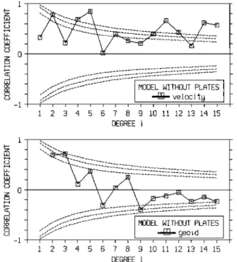
Figure 6 displays the correlation coefficients The power spectra of the computed surface ve- for each degree Z, between predictions and obser- locity field split into its poloidal and toroidal vations, both for the surface horizontal diver- components are depicted at the bottom of Figure gence (top) and the geoid (bottom) in the case of 8. The curves for the observed velocities are the model Earth without plates. For the plate plotted on the top for comparison. The general divergence, the meaningful correlations for de- trend and amplitude of the predicted powers are grees Z = 2, 4, and 5 are mainly related to upper highly satisfactory. We have chosen a reference mantle sources. For the geoid, only the degrees value for the upper mantle viscosity of
Z = 2 and 3 are significantly
correlated.
It is
2.6x10²ø Pa s in order to make the amplitudes of
well known that the lower mantle heterogeneities real and modelled spectra comparable. This yields deduced from seismic tomography explain this last a lower mantle viscosity of 1.3x10²² Pa s. observation. This correlation does not give any Figures 9 and 10 show the comparison between indication about the predicted amplitudes. The the observed (top) and computed (bottom) horizon- term which could induce the appropriate polar tal divergence and vertical vorticity, respect- flattening of the geoid is in fact too weak in ively. The existing plate motions are based on the tomography we used here. Other authors the global tectonics model of Minster and Jordan [Richards and Hager, 1985] using unpublished to-mography data [Clayton and Comer, 1983] found
much better agreement.
Z - Ld •-• _ Lu - LO _ o z co _ <E - Ld _ co - -1 Z - Ld •-• _ Lu - LO _ o z o _ H <]E - Ld _ -1 I I I I I I I I I I I [ I I I 1 2 3 'q 5 6 7 8 9 10 11 12 13 l'q 15 DEGREE 1
...•:f:•.%];]cC
...
ITI po
1
o i dal
-1 I I I I I I [ I [ I I I I I l 1 2 3 q 5 6 7 8 9 10 11 12 13 lq 15 DEGREE 1 Z - Ld • _ L• - LL LO _ o z o _ <E - Ld _ 0 - -1 •ODEL NZTH PLATESm õeo
i d
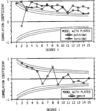
i i i I i ! I I I 7 8 9 10 11 12 13 14 15 DEGREE 1Fig. 7. Correlation coefficients between obser- vations and predictions for the velocity field Fig. 6. Correlation coefficients for each degree (top) and the geoid (bottom) when the 11 tectonic Z between observations and predictions for the plates are taken into account. By comparison with
poloidal
component of
the velocity
field
(top)
Figure 6 one sees the striking
increase of the
and the geoid (bottom). The case shown is for correlations, both for the lower degrees of the purely radial viscosity structure of an Earth geoid (bottom) and for all degrees of the polo- model, which is loaded with density heterogene- idal field (top, squares). Except for degree ities defined by seismic tomography and by slab Z = 2, the prediction of the toroidal field (top, seismicity. The three pairs of dashed curves re- circles) also shows a very good correlation with present confidence levels of 80, 90, and 95%. observations.17,550
Ricard and Vigny: Mantle Dynamics With Induced Plate Tectonics
1E+Ol '-,. 1E+OO-- LLI z 1E-01 - m,m 1E-02 - 1E-03 1E+81 OBSERVEDT ] poloidat
0
tonoidal
B Bmm DEGREE 1 ',. 1E+OO - ILl z 1E-01- H L• 1E-82- 1E-03 COMPUTEDITI poloidal
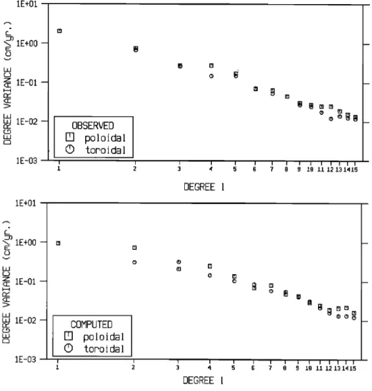
(]]) topo i dal i I 1415 DEGREE 1Fig. 8. The top graph depicts the power
spectra of the Earth's toroidal (circle) and
poloidal
(squares) velocity
fields derived from plate tectonics. This graph illus-
trates
the long recognized quasi-equipartition
of the observed plate motion between
the two modes. The prediction of our model is depicted in the bottom graph in the same
units (cm/¾r). The general trend is satisfactorily predicted. The toroidal components
of degree Z = 1 corresponding to the choice of an absolute reference frame for the velocity description have not been considered.
[1978] and are reconstructed up to degree Z = 15
In the previous figures we have shown
the two
using a previously published spectral decomposi-
components of the surface motion separately in
tion [Forte and Peltier, 1987]. The converging
order to emphasize the role of the existing
zones (Figure 9,
top) around the Pacific and
plates in the generation of toroidal flow. How-
above the Himalayan belt are depicted as light,
ever,
a direct
comparison with the well-known
whereas the fast spreading Nazca and East Indian
observed motions is obviously the best way to ap-
ridges are dark. Our predictions (Figure 9, bot-
preciate
the fit.
This is depicted in Figure 11.
tom} generally agree with observations. Never-
On top, the plate motions with harmonics
larger
theless an excessive opening of the North Indian than 15 removed are described in a reference
and Red Sea ridges is
induced by a very strong
frame where the toroidal motion of degree Z = 1
low-velocity
anomaly given by the upper mantle
is zero. At the bottom, our surface velocity pre-
tomographic model [Woodhouse and Dziewonski, diction is shown. There is a good resemblance be-1984]. Our simulation also underestimates
the
tween the two. The major discrepancy
comes
from
Aleoutian
subduction zone. For the observed vet-
the position of
the Pacific rotation pole which
tical vorticit¾ reconstructed without the degree is predicted too close to California. This misfitZ = 1,
which is
not predictable
by our model
was also revealed by the unrealistic
zero vorti-
(Figure 10, top), the right, respectively left,
city near the San Andreas
fault zone (Figure 10,
lateral
shears are shaded in dark, respectively
bottom).
light. The major shear zone North of Australia is
Let us now turn to the geoid (Figure 12). The
correctly
localized,
but the strike-slip
zone in
location
and amplitude of the main observed non-
California is not found by our prediction (Figure
hydrostatic geoid features (top) are present in
Ricard and Vigny: Mantle Dynamics
With Induced Plate Tectonics
17,551
/
,/
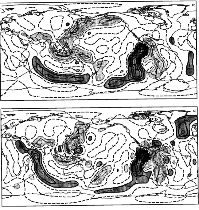
Fig. 9- Observed
(top) and predicted (bottom) divergence
of the surface
velocity
field.
The description is truncated beyond
degree g = 15 of the spherical harmonics.
In both maps, the level lines are 20x109
rad/yr apart. The maxima
are shaded
in dark
and the minima in light.
Despite some discrepancies, the global patterns are very
similar.
existing geoid
maxima
over
Africa, West
Pacific,
degree
and
order
have
a very low amplitude
in the
and Andes. The quality of the fit is comparable
tomographic data
to what has been obtained
for a more
complex
vis-
Another way to depict the fit between
obser-
cosity stratification and appropriate
density vations and
predictions is to plot the harmonic
anomalies but without plates [Ricard et al.,
coefficients of the computed
fields as a function
1989]. In terms of root-mean-square,
we only of the real ones.
This is done
in Figure
13: the
explain 22%
of the observed
signal
for degrees
Z
top for the divergence
and
vorticity together
and
between
2 and 15. The main
shortcomings
are the
the bottom
for the geoid. A perfect prediction
insufficient
polar flattening
and
the presence
of
would correspond
to all the points
lying on the
a strong minimum
over the Nazca
ridge. This diagonal
of each graph.
A reasonable
fit is at-
spurious
geoid
low
over
the East
Pacific
is rela-
tained,
with
noise
of about
74%
of the signal
for
ted to a too stong return flow induced
by the
the velocities
and
78%
for the geoid.
Taking
into
opening
of the ridge. The
polar
flattening
is
account
the simple
assumptions
of the model
and
mainly
described
by the spherical
harmonic
of de-
the uncertainties
that affect the tomography,
gree Z = 2 and order m = 0. Unfortunately,
as
this correlation
test seems
to be fulfilled. Of
17,552
Ricard and Vigny: Mantle Dynamics
With Induced Plate Tectonics
!
\
,,,..
Fig. 10. Same as Figure 9, but for the vorticity. The level lines are again 20x10
•
rad/yr apart. The sinistral shears
are shaded
in dark and the dextral ones
in light.
The amplitude and sign of shears between India-Australia and Pacific or between
Nazca
and Antarctica are well predicted. On the contrary, we miss the San Andreas
shear
zone. Nevertheless, the correlations between
the two maps
are very significant, as was
Ricard and Vigny: Mantle Dynamics With Induced Plate Tectonics
17,553
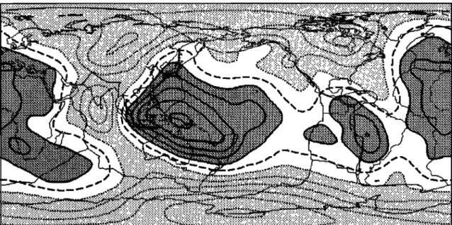
Fig. 11. The map at the top depicts the well-known Earth's plate motion filtered out for degrees Z > 15, the continental shore lines, and the plate boundaries. The map at the bottom is the result of our simulation at the same scale. The horizontal diver- gence and radial vorticity plotted on Figures 8 and 9 are associated with these two maps. In the usual hot spot frame, a rotation component would have been added which would have increased the Pacific motion and reduced the Eurasian and African motions.
17,554 Ricard and Vigny: Mantle Dynamics With Induced Plate Tectonics r.,..?,.• ,.,,'- __ ß q.•.-.'.'.-...:.:...'.-
•
% f..::iii::!:.:...
•.:::::.: ß --• • ",'.:.:.:.:.:.:.:.: ... -:.:-:.:.:.:.:-:-:., \ '•::::::::::::::: .... : .... ::.:... ß ... :..;. .•.,• .% ._•_•.,;.• ,,... •, ,• ß-•*'
•••'
'"••,,"•
•,,.;•J '-'•:"---'""•-'-•;;ii::ii;ii!::i{::".";.":'•i:i•..,....:..:
....:.:.:.:..•---,--...• 7 •"'"'" ',
% •,. •'",
-•
'--,I
===============================,..__•___-.--"
•=======================================================
...'"'•'''
'"'••:..
....•••::::i:::::•..."...-'..'-...'.,:.,.,...:.•-,...'"'"'"'•
""'
ß
========================================="---.•--'•-'---:="•-•-
-J
.,: ... ß ... :::::::::::::::::::::::::::::::::::::::::::: :Fig. 12. Observed (top) and predicted (bottom) geoid. The level lines are 20 m apart. Maxima and minima are again shaded in dark and light. Our model localizes the major features, but the fit is not as good as that for the velocities.