HAL Id: hal-00007490
https://hal.archives-ouvertes.fr/hal-00007490
Preprint submitted on 13 Jul 2005
HAL is a multi-disciplinary open access
archive for the deposit and dissemination of
sci-entific research documents, whether they are
pub-lished or not. The documents may come from
teaching and research institutions in France or
L’archive ouverte pluridisciplinaire HAL, est
destinée au dépôt et à la diffusion de documents
scientifiques de niveau recherche, publiés ou non,
émanant des établissements d’enseignement et de
recherche français ou étrangers, des laboratoires
SnIa Constraints on the event-horizon Thermodynamical
model of Dark Energy
Jérome Gariel, Gérard Le Denmat, Cécile Barbachoux
To cite this version:
Jérome Gariel, Gérard Le Denmat, Cécile Barbachoux. SnIa Constraints on the event-horizon
Ther-modynamical model of Dark Energy. 2005. �hal-00007490�
ccsd-00007490, version 1 - 13 Jul 2005
SnIa Constraints on the event-horizon
Thermodynamical model of Dark Energy
J. Gariel
∗, G. Le Denmat
†and C. Barbachoux
‡LERMA, UMR CNRS 8112
Universit´
e P. et M. Curie ERGA, B.C. 142
3, Rue Galil´
ee, 94 200 Ivry, France
Abstract
We apply the thermodynamical model of the cosmological event hori-zon of the spatially flat FLRW metrics to the study of the recent acceler-ated expansion phase and to the coincidence problem. This model, called “ehT model” hereafter, led to a dark energy (DE) density Λ varying as r−2, where r is the proper radius of the event horizon. Recently, an-other model motivated by the holographic principle gave an independent justification of the same relation between Λ and r. We probe the theoret-ical results of the ehT model with respect to the SnIa observations and we compare it to the model deduced from the holographic principle, which we call ”LHG model” in the following.Our results are in excellent agreement with the observations for H0 = 64kms−1M pc−1, and Ω0Λ = 0.63+0.1−0.01,
which leads to q0= −0.445 and zT ≃ 0.965.
Keywords: dark energy theory, supernova type Ia
1
Introduction.
Since the discovery of the presently accelereted expansion of the universe from supernovae observations [1][2], evidences for such an accelerated phase are in-creasing. The simplest theoretical candidate to explain this acceleration is a cosmological constant Λ. Anything producing sufficient negative pressure - for instance a scalar field [3] or a bulk viscosity [4] - could also be valid.
Before the discovery of this acceleration, phenomenological ansatze with a variable Λ(t) were tentatively proposed as solutions of the cosmological
“con-stant” problem. For instance, laws such as Λ(t) ∼ t−2 [5], Λ(t) ∼ a−2(t) [6][7],
where a(t) is the scale factor of the FLRW space-time, Λ(t) ∼ H2(t)[8] or
Λ(t) ∼ βH2(t) + (1 − β)H3(t)H−1
I [9], where H(t) is the Hubble parameter and
∗gariel@ccr.jussieu.fr †gele@ccr.jussieu.fr ‡barba@ccr.jussieu.fr
HI is its exponential inflation value, were suggested. Other proposals [10][11]
can also be quoted.
From a different point of view, the generalization [12] [13] of the black hole and of the de Sitter event-horizon Thermodynamics [14, 15] to the FLRW
space-time has led to the relation Λ(t) ∼ r−2(t) [16] where r denotes the event-horizon
in the FLRW model of the universe.
Recently, this last form for Λ(t), or, equivalently, for the dark energy
den-sity ρΛ(t) through ρΛ(t) = χ−1Λ(t) (with χ = 8πGc−4), has received further
confirmations based on the holographic principle [17, 18].
Let us remind of the approach which can been followed to produce a model with a time-dependent cosmological constant. We start with a type-like perfect fluid energy-momentum tensor
Tαβ= ρ
totuαuβ− Ptot∆αβ , ∆αβ= gαβ− uαuβ, (1)
where uα is the 4-velocity common to all the components of the energy
density ρtot. We consider two components such as ρtot = ρ + ρΛ and Ptot =
P + PΛ. The component (ρ, P ) is the matter with the barotropic state equation
P = (γ − 1)ρ where γ is a constant (for instance, γ = 1 for dust). The second
component is the Dark Energy (DE) with ρΛ, the vacuum energy density, and
PΛ the (negative) pressure satisfying the state equation
PΛ= −ρΛ. (2)
Relation (2) leads to the two following alternatives:
i) Each component is conserved separately and, of course, Λ has to be con-stant.
ii) Both of the components are conserved together, Λ = Λ(t) is then possible. The event-horizon Thermodynamics (ehT) model is derived on the basis of point ii) by assuming an interaction between the matter and the Dark Energy (DE hereafter). Let us remark that we write “matter” for any sort of matter except DE. Today, the matter is the dust, the largest part of which is the Dark Matter (DM). For sake of simplicity, we use DM to denote the dust, encompassing the baryonic matter. In the same vein, other models assuming an interaction between the DE and DM components of the cosmic fluid were studied, e.g. [19].
A model such that Λ ∼ r−2for the DE density can be used in different ways
and different contexts. For instance, in a precedent paper [16] in order to address the problem of the exit of inflation in the early universe, we imposed as second component a perfect fluid of strings (γ = 2/3). The model led then to Λ = 3..a
a, which was independently considered as an ans¨atz derived by dimensional
considerations by some authors [20] [21] [22]. An equivalence can be found
between the previous relation Λ ∼ ¨a
a and the forms Λ ∼ a−2 and Λ ∼ ρ under
In the present paper, in order to settle some issues on the coincidence and the recent decceleration-acceleration transition problems, we assume for the second component a cold dark matter (P = 0). In section 2 we review some basic equations and relations common to the ehT and LHG models. The ehT model is developed in section 3, particularly for the z ≤ 2 epoch. In section 4, in order to probe the DE assumption in this range of z, we discuss how our model fits in with the type Ia supernovae observations [24]. We deduce then the most likely
values for the H0 and Ω0Λ parameters, as well as the decceleration parameter q0
and the decceleration-acceleration transition redshift zT. Finally, sections 5 and
6 contain comments and a brief comparative discussion concerning the results obtained by the two models.
2
Model for
Λ and Field equations.
In order to set the notations, we introduce some basic equations of the two component models. The spatially flat FLRW space-time has the metric
ds2= c2dt2− a2(t)[dR2+ R2(dθ2+ sin2θdφ2)] (3)
where the scale factor a(t) is a monotonic increasing function of the cosmic time t.
We assume an universe filled by two interacting type-like perfect fluids, namely dust (ordinary and dark matter) and Dark Energy (DE). The dust and
DE energy densities are ρ and ρΛ = χ−1Λ respectively, and their
correspond-ing pressures are P and PΛ. The two state equations are P = (γ − 1)ρ with
γ = const, 0 < γ ≤ 2 , and PΛ= ωρΛ, where ω can be variable.
We recall the field equations for the spatially flat case
3H2= χc2(ρ + ρΛ) (4) 2 .. a a+ H 2 = −χc2(P + PΛ) , (5) where H ≡ a.
a is the Hubble parameter, c the velocity of the light and the dot
stands for the time derivative.
Combining these two equations leads to ˙
(H−1) =3
2(γ + (1 + ω − γ)ΩΛ) , (6)
where the dimensionless density parameter ΩΛ≡ Λc2/3H2has been introduced.
The equation (6) is always valid provided the DE is a perfect fluid.
We consider now Λ as a vacuum energy density associated to the FLRW event-horizon such as
Λ = 3α
2
where r is the proper radius of the event-horizon, and α is a dimensionless constant parameter. This form of Λ was previously obtained by [16] and [17] when α = 1, and by [18] when α 6= 1.
Using the quantity ΩΛ, relation (7) becomes
pΩΛ=
αc
rH . (8)
The proper radius of the flat FLRW event-horizon is r(t) = a(t)
Z ∞
t
c dt′
a(t′), (9)
The derivative of (9) with respect to time gives H − · r r = c r . (10)
For convenience, we introduce the variable x ≡ ln a(t) such as x = 0 today. Relation (10) becomes then
1 −r ′ r = c rH = √ ΩΛ α , (r ′ ≡ dr dx), (11)
where the prime means the derivative with respect to x. In the same manner, we can rewrite relation (6)
(H1)′
(H1) = 3
2(γ + (1 + ω − γ)ΩΛ). (12)
Finally, by combining equations (11) and (12) with the derivative of equation (8), one obtains
Ω′Λ= ΩΛ{3[γ + (1 + ω − γ)ΩΛ] − 2[1 −
√
ΩΛ
α ]} . (13)
Let us emphasize that this equation is valid for any values of γ (constant) and ω (constant or variable), independently of the fact that the two components ρ
and ρΛ are interacting or not.
It is useful to derive from the field equations (4) and (5) the decceleration parameter q q ≡ − ·· a aH2 = 1 2[(3γ − 2) + 3(ω + 1 − γ)ΩΛ]. (14)
which is valid in the two models.
In the following, we assume that the “matter” component ρ is dust (γ = 1), so that (13) and (14) become
Ω′Λ= ΩΛ(1 + 2
√
ΩΛ
q = 1
2(1 + 3ωΩΛ). (16)
The relations (3)-(16) are valid in the two models under consideration, which we denote Λ(t)CDM models hereafter.
From now on, the assumptions of the ehTmodel will be different from the LHG model’s ones.
3
Model with interacting components.
We assume that the DE component satisfies thermodynamical state equations, i.e. relations between its thermodynamical variables which are valid in any space-time. Therefore, any thermodynamical state equation valid in the de
Sitter’s space-time [15][25] - for instance, PΛ = −ρΛ and ρΛ = 12π2TΛ2 (TΛ
the temperature ) - remains valid in the FLRW space-time. Thus, if the DE is an actual cosmological component, its thermodynamical state equations will stay the same, independently on the choice of the space-time as well as for any other component. This suggests to retain the relation (7) which is valid in the de Sitter’s space-time when α = 1. In section 5, some consequences of the presence of the parameter α in the ehT and LHG models are discussed. Using the holographic principle can lead also to choose the relation (7) [17], [18]. These references assume a variable state equation (ω = ω(x)) for the DE, and independent energy conservation laws for the matter and DE components. Conversely, the present model assumes ω = −1 (vacuum), and that the energy conservation is only valid for the two components considered together.
Equation (15) can be rewritten Ω′
Λ= 3ΩΛ(β2−pΩΛ)(β1+pΩΛ) (17)
where the constants β1and β2 are given by
β1≡ 1 3α( p 1 + 3α2− 1) , β 2≡ 1 3α( p 1 + 3α2+ 1), β 1, β2> 0. (18)
By setting α = 1, Equation (17) becomes Ω′
Λ= ΩΛ(1 −pΩΛ)(3pΩΛ+ 1), (19)
which differs from Equation (8) in [19]. Nevertheless a straightforward
calcula-tion (using (12),(15) and the derivative of the definicalcula-tion of ΩΛ) gives
Λ′= 2Λ(pΩ
Λ− 1) , (20)
which is common to the two models. As Λ′ is always negative, Λ is decreasing
with time. Observational evidences provide a very small present value for ρΛ
Introducing the function y(x) ≡√ΩΛ, Relation (17) becomes
2y′ = 3y(β
2− y)(β1+ y). (21)
Its solution is (in the only case considered here where y < β2)
K1a = y2 (β2− y) α β2√1+3α2(β 1+ y) α β1√1+3α2 . (22)
K1 is a constant of integration which can be related to the initial condition
y0=pΩ0Λ.
We derive now the expression of r = r(y). Using Equations (11) and (21) yields
d(ln r) = dx −3α(β 2dy
2− y)(β1+ y)
. (23)
After integration, one obtains
K2r = a(β2− y β1+ y) 1 √ 1+3α2 (24) or equivalently Kr = y 2 (β2− y) α−β2 β2√1+3α2(β 1+ y) α+β1 β1√1+3α2 , K ≡ K1K2. (25)
K2is a second constant of integration which depends on y0and r0= αc(y0H0)−1.
The expressions of K1 and K2 depend explicitly on the two priors Ω0Λ and H0.
The current values of Ω0
Λ and H0 are Ω0Λ = 0.7 and H0 = 72 km.s−1.M pc−1
[26]. With these two numerical values, it is interesting to deal with the case
where α = 1 for which β1=13 and β2= 1. One obtains
K1a = y2 (1 − y)12(1 3+ y) 3 2 , K1= y2 0 (1 − y0) 1 2(1 3+ y0) 3 2 = 1.3686 (26) K2r = a(1 − y1 3+ y )12 , or Kr ≡ ( y 1 3+ y )2, r0= c H0y0 = 4980.12M pc (27) K2 = 1 r0 (1 − y1 0 3+ y0 )12 = 7.50265 × 10⁻⁵M pc−1, K = 1.02681 × 10⁻⁴M pc−1.
However the previous values of H0 and Ω0Λ are model-dependent. They were
obtained in the framework of the ΛCDM model. We shall see that starting with the same observational SnIa data, the best fit to the Λ(t)CDM models
4
SnIa constraints on the ehT model
In order to compare these theoretical results with the observations of the SnIa
magnitudes, the luminosity distance dL has to be expressed with respect to the
redshift z = a−1− 1. In the ehT model, it yields
dL= (1 + z)[(1 + z)r − r0] = c(1 + z) y0H0 [(1 + z)r r0 − 1], (28) where the expression of r depends on z. As before, we only consider the case α = 1. Both Equations (22) et (25) give a parametric representation (via the “parameter” y) of r as function of z. Indeed, (22) yields immediately z = z(y)
(with a = (1 + z)−1).
The set of the theoretical curves “distance moduli” µ versus the redshift z,
µ ≡ m − M = 25 + 5 log10(dL) , with dL in Mpc, (29)
predicted by the model parametrized by the two cosmological parameters y0=
pΩ0
Λ et H0, can be plotted. For the two parameters Ω0Λ and H0 free, the best
fit to the magnitude observational data of the 157 SnIa “Gold sample” [24]
can be determined by minimizing the function χ2 = P(µ(z)−µi(zi)
σi )
2, where
µi(zi) denotes the values of the magnitude for the observational data, σi the
corresponding error and the summation is taken over any of the 157 data of
the sample. The corresponding values of Ω0
Λ and H0 are derived by numerical
computation. More precisely, Equation (21) is integrated by the method of Runge-Kutta of order 4, and the expression of z(y) is deduced by use of (22). With the help of Equations (28) and (29), the values of µ(z) for z ranging
from 0 to 100 are then obtained. After a simple numerical evaluation of χ2for
Ω0
Λ ranging from 0 to 1 and H0 from 50 to 100, the best fit corresponding to
χ2= 178, 7 is obtained for
H0= 64+7−4km.s−1.M pc−1, Ω0Λ= 0.63+0.1−0.01, (30)
The function µ(z) is plotted in figure 1 for z ranging from 0 to 2.
The likelihood function L(Ω0
Λ) (see figure 2) is derived by marginalization of
H0 and furnishes the same value of the parameter Ω0Λ.
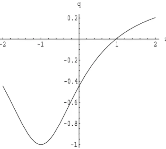
Finally, the decceleration parameter q can be expressed as a function of y in the ehT model ( for α = 1) from equation (16) ( with ω = −1)
q = 1
2(1 − 3y
2). (31)
In figure 3 the curve q(z) of the ehT model is plotted. Today the
decceler-ation is q0= −0.445 , and the decceleration-acceleration transition occured at
30 35 40 45 50 0 0.5 1 1.5 2 MU z
Figure 1: The “distance moduli” µ(z) of the ehT model
5
The event horizon and the parameter α.
We examine here the influence of the parameter α on the limits of the proper radius r of the event horizon (eh) in the two models. First, let us consider the LHG model.
By comparison with the relations (22) and (25) of the ehT model, the LHG model would lead to the relations ( a is given by (9) of [18] and r, not explicitly given, can be deduced from their eqs. (6) and (9)):
Y0a = y2(1 + y) α 2−α (1 − y)2+αα (α + 2y) 8 4−α2 , α 6= 2 , Y0= y2 0(1 + y0) α 2−α (1 − y0) α 2+α(α + 2y0) 8 4−α2 , (32) r = α Y 3 2 0 H0p1 − Ω0Λ y2(1 + y)1+α2−α(1 − y)1−α2+α (α + 2y)4−α212 . (33)
For α = 2, the LHG model requires to start again the calculation from the differential equation (15) which becomes:
2y′= y(1 − y)(1 + y)2. (34)
Its integration yields
a =(1 − y0) 4 3(1 + y0) 2 3 y2 0 y2 (1 − y)43(1 + y) 2 3 exp(8 3( 1 1 + y − 1 1 + y0)). (35) Then, r = 2c(1 − y0) 2(1 + y 0) H0p1 − Ω0Λy03
y2exp(1+y4 −1+y40)
(1 − y)32(1 + y) 1 2
0 0.2 0.4 0.6 0.8 1 0 0.2 0.4 0.6 0.8 1
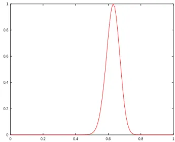
Figure 2: The likelihood function L(Ω0
Λ) of the ehTmodel
We can see from (33) or (36) that a tends to infinity when y tends to 1, for any values of α (positive, see (8)). But the behaviour of r differs because it depends on the parameter α, as it can be seen from (32) and (35). Three cases can be distinguished for the behaviour of r in the limit y → 1:
r → 0 if α < 1 (37) r → ∞ if α > 1 (38) r → ri= cst = ( 2 9) 2 c H0p1 − Ω0ΛY 3 2 0 = r0(2 9 (1 + 2y0)2 (1 + y0)y0) 2 ≡Hc i if α = 1. (39) The first two cases ( i.e. r → 0 and r → ∞ ) disagree with the holographic point of view, because they would prevent any cut-off (IR and UV respectively). In particular, the case α < 1 seems to be proscribed because it could not prevent the singularity formation and would correspond to the absence of black hole formation .
The third case only (α = 1) corresponds to a de Sitter asymptotic limit. In Equation (39), the index i of H means exponential “inflation”. Note that the limit ri
r0 depends only on y0, and its value is :
ri
r0 = 1.06813 if we take y0=
√ 0.7.
As r0 = H0cy0 = 4980.12M pc, ri is equal to 5319.42M pc. The expression of r0
is formally the same in the two models and depends only on the choice of the
observationnal priors H0et y0. However, each model leading to slightly different
-2 -1 1 2 z -1 -0.8 -0.6 -0.4 -0.2 0.2 q
Figure 3: The decceleration parameter q(z) of the ehTmodel
In the case of the ehT model, for any arbitrary α, the same phenomenon appears and the value α = 2 does not necessitate a special study. In the limit y → 1, Equations (26) and (27) give
a → ∞ and r → 0 if α < 1 (equivalently, β2 > 1)
a → ∞ and r → cst = K1 (3
4)
2= 5478.13M pc if α = 1 (equivalently, β
2= 1)
When α > 1, β2< 1, then y → β2before reaching 1, and a → ∞ , while r → ∞
for this asymptotical limit β2 of y. From the today observational evaluations,
β2 has to be >
√
0.63 = 0.79, and so α < 3×O.63−12√0.63 = 1.78. In the future, α
range from 1 to 1.78 will become more and more narrow, tending to 1, as long
as the equation (17) of the model, indicating a growth of ΩΛ, remains valid.
Thus, the case α = 1 appears to us as the most attractive. The corresponding
de Sitter’s limit is ri = 5478.13M pc. It is a little greater than the limit of the
LHG model (5319.42M pc), which means a little weaker exponential inflation.
6
Conclusion.
We have seen that the form Λ ∼ r−2, clearly supported by the holographic
principle, leads, in our study, to two somewhat different models, owing to the chosen energy conservation equation. In the ehT model, α = 1 and the best fit (χ2
ν = 1.14) to the SnIa’s data from the “gold” sample [24] gives us H0 = 64
km.M pc−1.s−1 and Ω0
Λ = 0.63. If α 6= 1 (as in the LHG model) it is worth
observing that the α < 1 values are not very attractive because they lead to the
singularity r → 0 when ΩΛ→ 1.
For the decceleration-acceleration transition epoch we find a redshift zT =
0.72)[18] [24] and very sensitive to the Ω0
Λ value. Comparing the values of
the cosmological parameters in various models requires to discuss not only the choice of the parameter α but also the forms or relations taken for q(z) (for
instance, q(z) = q0+ q1z valid when z ≪ 1), for ω(z), or for dL(z). Besides, in a
given model, one has to take into account the energy conservation laws for DM and DE. In most cases, the authors assume an energy conservation law for each component separately. Here we have considered the more general situation of a global conservation of the whole energy and, necessarily, an interaction between DM and DE. Such an interaction could induce higher values for the transition
redshift zT, as noted by Amendola et al. for models with coupling [27, 28].
Fu-ture observations in the high redshift range could allow to discriminate between theories with coupled components and theories with distinct conservation laws.
References
[1] A.G. Riess, Astron. J.116 (1998) 1009. [2] S. Perlmutter et al., Nature 391 (1998) 51.
[3] B. Ratra and P.J.E. Peebles, Phys. Rev. D 37 (1988) 3406. [4] G.L. Murphy, Phys. Rev. D 8 (1973) 4231.
[5] K. Freese, F.C. Adams and J.A. Frieman, Nucl. Phys. B 287 (1987) 797.
[6] M. ¨Ozer and M.O. Taha, Nucl. Phys. B 287 (1987) 776.
[7] W. Chen and Y.S. Wu, Phys. Rev.D 41 (1990) 695.
[8] J.C. Carvalho, J.A.S. Lima and I. Waga, Phys. Rev. D 46 (1992) 2404. [9] J.A.S. Lima, J.M.F. Maia, Phys. Rev. D 49 (1994) 5597.
[10] E. Gunzig, R. Maartens and A. Nesteruk, Class. Quantum Grav. 15 (1998) 923.
[11] I. Prigogine, J. Geheniau, E. Gunzig and P. Nardone, Gen. Rel. Grav. 21 (1989) 767.
[12] P.C.W. Davies, Class. Quantum Grav. 5 (1988) 1341
[13] M.D. Pollock and T.P. Singh, Class. Quantum Grav.6 (1989) 901. [14] J.D. Bekenstein, Phys. Rev. D 7 (1973) 2333.
[15] G. Gibbons and S.W. Hawking, Phys. Rev. D 15 (1977) 2738. [16] J. Gariel and G. Le Denmat, Class. Quantum Grav.16 (1999) 149. [17] M. Li, Phys Lett B (2004) 603.
[18] Q.G. Huang and Y. Gong, J. Cosmol. Astropart. Phys. JCAP 08 (2004) 006.
[19] D. Pavon, S. Sen and W. Zimdhal, Preprint [astro-ph/0402067] (2004). Olivares G, Atrio-Barandela F and Pavon D, Preprint [astro-ph/0503242] (2005).
[20] J.M. Overduin and F.I. Cooperstock, Phys. Rev. D 58 (1998) 043506. [21] A. Pradhan, G.S. Khaledar and D. Srivastava, Preprint gr-qc/056112
(2005).
[22] A.I. Arbab, J. Cosmol. Astropart. Phys. JCAP 05 (2003) 008. [23] S. Ray and U. Mukhopadhyay, Preprint [astro-ph/0407295] (2004). [24] A.G. Riess et al., Preprint [astro-ph/0402512] (2004).
[25] M. Gasperini, Class. Quantum Grav. 5 (1988) 521. [26] D.N. Spergel et al., Preprint [astro-ph/0302209] (2003). [27] L. Amendola, MNRAS 32 (2003) 221.
[28] L. Amendola, M. Gasperini and F. Piazza, Preprint [astro-ph/0407573] (2004).