Damage detection in civil and aerospace structures with fiber optic sensors

(1)

Damage Detection in Civil and Aerospace Structures with.

Fiber Optic Sensors

by

Niell Glen Elvin

Bsc. Engineering, University of the Witwatersrand Johannesburg, South Africa (1994)

Submitted in partial fulfillment of the requirements for the degrees of Master of Science in Civil and Environmental Engineering

and

Master of Science in Aeronautics and Astronautics at the

MASSACHUSETTS INSTITUTE OF TECHNOLOGY

September 1995

A uthor ... - = . .. ...

Department of Civil and Environmental Engineering

and. Department of Aeronautics and Astronautics

August 11, 1995

Certified by ... ... ,.. ... . ... ... ... ... Assistant Professor Christopher K. Y. Leung

, /- /Thesis Supervisor

Certified by...

. ...

...

Professor Paul A. Lagace

Thesis Supervisor

A ccepted by ... ... . ... . ...

S/ Professor Harold Y. Wachman

Chairman. Department Graduate Committee

- ,, DiD rtent of Aeronautics and Astronautics

A ccepted by ... ... ...

Professor Joseph Sussman Chairman. Department Committee on Graduate Students Department of Civil and Environmental Engineering .. A.AC-•US- fT'S INS' 'i' (L

OF TECHNOLOGY

OCT

25 1995

(2)

Damage Detection in Civil and Aerospace Structures with

Fiber Optic Sensors

by

Niell Glen Elvin

Submitted to the Department of Civil and Environmental Engineering and

Department of Aeronautical and Astronautical Engineering on August 11, 1995, in partial fulfillment of the

requirements for the degrees of

Master of Science in Civil and Environmental Engineering and

Master of Science in Aeronautical and Astronautical Engineering

Abstract

The objective of this research is to investigate the performance of fiber optic sensing schemes that can accurately and reliably monitor the integrity and state of dam-age in civil and aerospace structures. The work presented in this thesis focuses on developing the combined electromagnetic and mechanical analysis required to study the behaviour of fiber optic sensing for two specific applications: (1) locating and monitoring tension cracks in concrete structures, and (2) detection of delamination cracks in composite and concrete structures.

Microbend fiber sensors that bridge the faces of tension cracks in concrete are studied as a possible means of determining the existence and extent of common damage in concrete structures. Delamination damage characterization by birefringent and in-terferometric sensors positioned parallel to delamination damage in typical aerospace composites and concrete structures is also investigated.

(3)

The microbend tension crack sensor was found to be able to detect cracks in the 0.01 mm crack opening range which makes them ideal for inspection of concrete struc-tures. The study of delamination damage sensors showed the ability of these sensors to detect delamination crack lengths in the 1 mm rang making them suitable for monitoring delaminations in advanced composite flexural members. The delamina-tion sensors investigated in this research have also shown potential use for structural integrity monitoring in reinforced concrete structures with 0.1 meter delamination lengths being detectable.

Thesis Supervisor: Christopher K. Y. Leung

Title: Assistant Professor of Civil and Environmental Engineering Thesis Supervisor: Paul A. Lagace

(4)

Acknowledgments

This thesis is a tribute to all those who on hearing that I was doing a joint degree in civil and aerospace engineering remarked : 'What do you do, design runways ?' To my knowledge this is the first attempt (at least at MIT) of doing a joint degree in two such diverse branches of engineering. I hope that my effort warrants interest from others since I beleive that there are important lessons to be learned from both sides.

For the opportunity of working in two departments, their interest, opinions and unique perspectives of the civil and aerospace industries I thank my supervisors Chris Leung and Paul Lagace.

I am as always grateful to the continued support of my parents through my long acedemic career. My brother deserves special thanks for being both a good friend and for providing invaluable advice. I recognize that without my family's help this thesis would not appear in its present form if at all.

(5)

List of Figures

2-1 Geometric propagation of EM waves along a curved optic wave guide. 37 2-2 Physical model of a slab waveguide. ... . . . . 37 2-3 An array of lenses equivalent to the beam propagation expressed in

Equation (2.32

).

. . . .

. . . .. .

38

2-4 Refractive index profile and normalized input electric field for a mono-mode step index slab wave guide ... 38 2-5 Electric field attenuation at discrete distances for a constant curvature

wave guide. Radius of curvature is 8 mm... 39 2-6 Electric field attenuation for various constant radii of curvature.

Prop-agation length = 5 mm ... 39 2-7 Rate of power attenuation for various constant radii of curvature. . . 40 2-8 Comparison of theoretical solution obtained by Marcuse and BPM

re-su lts . . . . 40 2-9 Rate of power attenuation through S - curve of various radii... 41 3-1 Physical model of oblique fiber bridging Mode I crack. . ... 53 3-2 Equivalent physical model showing prescribed transverse and

longitu-dinal displacements. ... ... . 53 3-3 Finite element model of fiber bridging crack faces ... . . . 54 3-4 Detail of finite element mesh at the fiber matrix connection. ... 55 3-5 In-plane, a, and ay, stresses in a jacketed fiber at one fiber diameter

from the crack face ... 55 3-6 In-plane, a, and ay, stresses in a fiber without jacket. . ... 56

(9)

3-7 Comparison of deflected shape between fiber center-line, outer radius

and jacket matrix interface. ... .. 56

3-8 Fiber Deflected shape for the case of jacket free fiber. . ... . 57

3-9 In-plane, a, and ay, stresses in a jacketed fiber at two fiber diameters from the crack face ... ... 57

3-10 Stress concentration at the debonded zone . ... 58

3-11 Radius of curvature along fiber center-line. . ... . . 58

3-12 Beam on elastic foundation model of an embedded fiber in an elastic m atrix .. . . . .. . . . ... 59

3-13 Beam on elastic foundation model for an oblique embedded fiber in an elastic m atrix . . . . 59

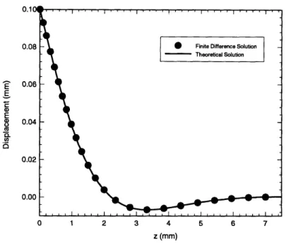
3-14 Comparison of Finite Difference and theoretical solution for beam on a linearly varying foundation stiffness, 3. . ... 60

3-15 Comparison of Finite Element and Finite Difference results for the center-line deflection of the fiber with various assumed stiffnesses, P. . 60 4-1 Effect of Crack Opening Displacement and fiber orientation on electric power attenuation by the finite element method (FEM) and the finite difference method (FD) ... ... 69

4-2 Effect of Jacket Elastic Modulus on electric power attenuation... 69

4-3 Effect of Cut-off Frequency on electric power attenuation... . 70

6-1 Physical elasticity model of weakened cantilever beam. . ... . 109

6-2 Comparison of derived theoretical solution with Savin's solution for the normalized tangential Stress _QhJ on the hole edge. . . . .2 109 6-3 Boundary Element Model of weakened cantilever beam ... 110

6-4 Comparison of BEM and theoretical solutions (a,) at various distances from the elliptic hole ... ... 111

6-5 Comparison of BEM and theoretical solutions (ay) at various distances from the elliptic hole .. .... ... ... ... .. ... .. 112

(10)

6-6 Comparison of BEM and theoretical solutions (a,,) at various distances

from the elliptic hole... 113

6-7 Rotation of Birefringent axes due to applied stress. . ... 114

6-8 x, Sensitivity map at sensor position f/h = 0.1 . ... 115

6-9 e~ Sensitivity map at sensor position f/h = 0.1 . ... 115

6-10 E,, Sensitivity map at sensor position f/h = 0.1 . ... 115

6-11 Effect of sensor position on theoretical sensor reliability. ... 116

6-12 Effect of finite beam depth on Ex sensor reliability. ... . . 116

6-13 Effect of finite beam depth on eY sensor reliability. . ... 117

6-14 Effect of finite beam depth on E,, sensor reliability. . ... 117

6-15 Effect of crack length (2a) on sensor reliability. Normalizing parameter is the maximum shear sensitivity component ... 118

6-16 Schematic layout of laminated cantilever beam. . ... 119

6-17 Allowable applied load of [Om/ ± 45,/90k]s laminate. k = 100-m-2n . 119 6-18 Engineering elastic modulus of [Om/ ± 45,/90k]s laminate. k = 100-m-2n120 6-19 Load to elastic modulus ratio for all n of [Om/ ± 45,/90k], laminate. k = 100-m -2n . . . 120

6-20 Effect of crack length (a) on the strain difference (6E) for delaminated beam. Crack position at beam mid-point c = 62.5 mm and d = 0. Fiber position at f = 0.8 h = 10 mm. ... 121

6-21 Effect of crack length (a) on the strain difference (fEy) for delaminated beam. Crack position at beam mid-point c = 62.5 mm and d = 0. Fiber position at f = 0.8h = 10 mm. . ... 121

6-22 Influence line for normalized sensitivity (6cy). Crack Length a = 1 mm. Crack Position c = 62.5mm. Fiber position at f = 22.5 mm. Normalizing sensitivity given by Calero sensor of 5uE over 152 mm. . 122 6-23 Normalized stresses under point load acting on unweakened beam. Normalizing factor taken as the maximum stress. . ... . . 123

(11)

6-24 Normalized stress difference between cracked and uncracked beam sub-jected to point load. Normalizing factor equal to maximum stress

dif-ference. ... 124

6-25 Influence lines for normalized sensitivity (&6y) for various crack heights d/h. Beam height h = 25 mm. Crack Length a = 1 mm. Normalizing sensitivity given by Calero sensor of 5pE over 152 mm. . ... 125

6-26 Influence lines for normalized sensitivity for various crack lengths a. Crack position c = 62.5 mm. Crack depth d = 0 mm. Normalizing sensitivity given by Calero sensor of 5pe over 152 mm. . ... 125

6-27 Influence lines for normalized sensitivity (~y) for two cracks. Crack positions at cl = 31.25mm and c₂= 93.75mm. Crack depths at d = Omm. Crack lengths a = 1mm. Normalizing sensitivity given by Calero sensor of 5pe over 152 mm .... ... . . . 126

6-28 Schematic representation of a moving load test for an aircraft component.126 6-29 Reinforced concrete cross section. . ... . 127

6-30 Reinforced concrete beam and sensor layout. . ... 127

6-31 Effect of crack length (a) on the strain difference (6E) for delaminated concrete beam. Crack position at c = 2 m and d = 0.165 m . Fiber position at f = 0.8 h = 0.152 m... .. 128

6-32 Effect of crack length (a) on the strain difference (6,y) for delaminated concrete beam. Crack position at c = 2 m and d = 0.165 m . Fiber position at f = 0.8 h = 0.152 m... ... 128

6-33 Influence lines for normalized sensitivity (6cy) for a simply supported beam. Crack position at c = 2m. Crack depths at d = 0.165 m. Fiber position at f = 0.8 h = 0.152 m. Normalizing sensitivity given by Calero sensor of 5pc over 152 mm... 129

A-1 Input fundamental mode for a straight slab waveguide. . ... 137

A-2 Input and transformed waveguide index. . ... . 137

(12)

A-4 Ouput electric field after propagation of 3 mm in a 5 mm radius of curvature fiber. ... 138

(13)

Notation

-

Electromagnetic analysis

a Radius of optical fiber core. c Speed of light in vacuum. B Magnetic flux density vector. D Electric flux density vector.

E Electric field intensity vector.

Ei Electric field intensity vector component in i direction. EM Electromagnetic.

H Magnetic field intensity vector. J Current density vector.

ki Wavenumber in medium i, i = 0 corresponds to vacuum. NA Numerical aperature.

ni Refractive index of medium i, i = 0 corresponds to vacuum.

P Poynting vector.

r Axial distance from core center. TE Transverse Electric Waves.

u Eigenvalue of slab waveguide core. v Normalized (or cut-off) frequency. w Eigenvalue of slab waveguide cladding. a Power attenuation loss.

P Propagation constant.

Ei Magnetic permittivity of material i, i = 0 corresponds to vacuum. A Wavelength.

Ao Magnetic permeability of free space.

0a Magnetic conductivity of material i, i = 0 corresponds to vacuum.

(D Time invariant electric field intensity vector. Direction invariant electric field intensity.

w Wave frequency.

(14)

Notation - Mechanical analysis

If Fiber free length. R Fiber radius.

t Fiber jacket thickness. u Crack opening displacement.

/~ equivalent foundation modulus.

6 Fiber-tip displacement.

(15)

Notation

-

Delamination Analysis

a Major ellipse half axis. b Minor ellipse half axis.

c Crack position coordinate (x-direction). d Crack position coordinate (y-direction).

E Young's modulus.

f Fiber sensing position (y-coordinate). FPF First Ply Failure Load.

h Half beam depth.

J Second moment of area of the beam.

k Number of 900 plies in [Om/ ± 45,/90k], laminate. 1 Beam length.

m Number of 0O plies in [Om/ ± 45n/90k], laminate.

n Number of ±45' plies in [Om/ ± 45,/90k], laminate.

Q Total applied tip force. U Airy stress function.

Uo Airy stress function for uncracked member.

6E Strain difference between cracked and uncracked member.

AE Absolute integral of weakened to unweakened strain difference.

Ei Strain component in the i-direction.

V) Complex analytical stress function.

X Complex analytical stress function.

v Poisson's ratio.

(16)

Chapter 1 Introduction

In the U.S alone, billions of dollars per year are spent on the inspection and repair of existing structural components. In concrete structures, the high cost of structural repair is due partly to the cost of manual inspection and the lack of reliable techniques for detection of damage at an early age. In advanced composites, the non-destructive evaluation techniques which are used for damage monitoring tend to be expensive and unreliable. Fiber optic sensors can potentially offer a solution to existing structural integrity monitoring problems due to their high sensitivity, low weight, immunity to electromagnetic interference such as lightning, continuous monitoring capabilities, their ability to detect distributed strains and their relatively cheap price. Another advantage of fiber optic sensors is the relative ease with which they can be embedded into curing materials such as reinforced concrete and advanced composites, which makes them ideal for integrity monitoring in civil and aerospace structures.

Previous work in structural damage sensor assessment has concentrated on exper-imental determination of sensor reliability under conditions in which the position and extent of damage is known. In practice, the location and extent of the damage is un-known and can greatly influence the ability of previously proposed sensing schemes to detect the damaged zone. This work focuses on theoretical and numerical electro-mechanical analysis to provide guidlines for the design and placement of fiber optic sensors. The factors effecting fiber optic system design are (a) crack length (or

(17)

open-ing), (b) relative position of the fiber sensor to the crack, (c) orientation of the fiber relative to the damaged zone, (d) mechanical properties of the fiber and structural material and (e) optical properties of the fiber.

The sensing of two typical failure modes in civil and aerospace structures are studied in this work. In particular, the feasibility of using fiber optic sensors to detect (a) ten-sion cracks in concrete structures, (b) delamination damage in advanced composites and in reinforced concrete structures.

The first four chapters of this work deal with the evaluation of the combined electro-magnetic and mechanical behaviour of micro-bend fiber optic sensors used for tension damage detection. The key parameters required for successful optic sensor design are identified and their effects on sensor performance are investigated. Chapter 2 explains the electromagnetic concepts required for the investigation of light wave propagation through optical waveguides and presents the Beam Propagation Method which allows the modelling of wave propagation through arbitrary sensor geometry. Chapter 3 fo-cuses on presenting the mechanics of crack bridging fibers using three-dimensional finite element analysis and beam on elastic foundation models. Chapter 4 and 5 com-bines the electromagnetic and mechanical analysis to investigate the effects of various material and geometric parameters on crack sensor performance. Chapter 6 concludes the section on tension crack detection by explaining the parameters required for suc-cessful fiber optic sensor design.

Chapter 7 focuses on the feasibility of using fiber optic strain sensors for delami-nation detection by monitoring changes in strain caused by delamidelami-nation, formation and growth. Effects of various parameters on crack detectability are investigated in this section. Two case studies are presented to show the applicability of fiber sensors in delamination detection for advanced aerospace composites and similar debonding damage in reinforced concrete structures.

(18)

The conclusion of the thesis outlines the research undertaken and presents the aims of future research.

(19)

Chapter

Electromagnetic Wave

Propagation

2.1 Optical Wave guide Basics

2.1.1 Basic Electromagnetic Definitions

This section develops some of the basic electromagnetic concepts used further in this thesis.

An electromagnetic wave traveling in medium i, has speed, ci given by :

A2w

= 27r

The frequency of propagation is related to the wave number k by :

k =

-CO

The refractive index of a material is given by the ratio of light velocities :

CO ni - --ci

(2.1)

(2.2)

(2.3)

(20)

where co is the velocity of light in vacuum and is given by :

1

2 = (2.4)

The light velocity in a non-magnetic medium is given by :

c =

i _-LO-

(2.5)

Using equations (2.3) to (2.6) it can be shown that :

Eo i (2.6)

ni

Substituting equations (2.3) and (2.5) into equation (2.2) and squaring gives :

k2 = W J (2.7)

ni

2.1.2 Wave Guide Definition

Any optical device which is able to guide electromagnetic energy in the optical fre-quencies along a well-defined path is known as an optical wave guide.

Essentially any medium consisting of a transparent dielectric material of low opti-cal loss can serve as a transmission medium for guided optiopti-cal waves if the refractive index of the material on the outside of the wave guide is less than the refractive index on the inside.

2.1.3 Wave Guide Characterization

Commercially available optical wave guides consist of a central core made of glass or plastic dielectric through which most of the electromagnetic energy is transmitted. The core is surrounded by a different dielectric material whose refractive index is slightly (less than 0.5%) lower than that of the core. The little electromagnetic field which is carried in the cladding decays rapidly to zero with distance from the core.

(21)

Figure (2-1) shows the geometric representation of a mono-mode EM wave propa-gating in a bent step refractive index optic wave guide. Note that electro-magnetic energy is lost through the cladding in the bend.

In Figure (2-1), the following symbols are used :

ni Refractive index at fiber center.

n2 Refractive index of cladding.

a Diameter of core.

2.2 Analysis of EM Transmission in a Slab Wave

Guide

This section describes the analysis of a straight slab wave guide. Circular fiber trans-mission is not considered since as shown in section (2.6), circular fiber behaviour is computationally and mathematically more difficult to model than slab wave guide behaviour but can be approximately modelled by changing the material characteris-tic in the slab wave guide analysis. [6]

EM wave guide propagation theory has its roots in Maxwell's equations:

aB

OH

V x E =--=

o

(2.8)

at

aD

dE V x H = + J = Ei + aiE (2.9)

at

The magnetic field vector, H, can be eliminated from these two equations by taking the curl of equation (2.8), to give :

X V

(22)

Expanding the left hand side of equation (2.10) with standard vector calculus tech-niques and substituting equation (2.9) into the right hand side leads to :

02E

OE

V(V * E) - V2E = -0Ei _at22 - P0o

a

at

(2.11)

In the case of propagation through an homogeneous, isotropic medium with no free charge, V * E = 0, the wave equation can be rewritten as :

a2E OE

VWE = Ioi--

W atd

+ 0o t (2.12)

Equation (2.12) is solved by assuming harmonic wave propagation in the z -direction. Hence every component of the electric and magnetic field is then given by :

5 = E(x, y, z)eiwt

(2.13)

Assuming that the medium is into equation (2.12) gives :

lossless gives oi = 0 and substituting equation (2.7)

(V 2 _{+ k2n}_{)l = 0} (2.14)

In the case of an electric field Maxwell's Equation reduces to

propagating along one direction, say the z direction, the Helmholtz equation.

(V2 + k2n)(Dz = 0

(2.15)

In general the Helmholtz Equation needs to be solved to find the the electric field distribution in 3 dimensions in an optical wave guide. The next section deals with solving the Helmholtz equation.

(23)

2.3 Solution of the Helmholtz Equation by the

Beam Propagation Method

A general algebraic solution of the Helmholtz equation is not possible. Various nu-merical tools including, finite-difference [14], effective-index [7], Rayleigh-Ritz [15] and hybrid methods have been proposed. Lately the Beam Propagation Method (BPM) has had increasing success with more than 20 articles being written on the subject in 1994 alone. The BPM was first proposed by Fleck et al. (1976) [4] for the solution of high energy laser beam propagation but has since been extended to the solution of propagation of EM waves in any medium with small variations in refractive index. The traditional BPM relies on two assumptions :

(1) The field propagates along only one direction, the z axis with no backward trav-eling field.

(2) The field can be considered paraxial, that is the optical rays essentially propagate along the central axis of the wave guide. This condition is realized when there are no abrupt changes in wave guide geometry, wave guide indices or wave guide curvature.

Under these conditions, the stationary electric field IP is given by :

I(x,

y,

z)

=

/(x,

y,

z)e

- j o_knaz,

_(2.16)

The Helmholtz equation (2.15) can be rewritten as a parabolic equation in q :

ao

₌- _j.VT + k2(n2 - n )

n (x, y, z) _(2.17)

az 2nak

where VT + 2 and the term _ is ignored due to the Fresnel assumption of

no rapid fluctuations in electric field. The Fresnel assumption is valid when there are no abrupt changes in fiber geometry.

Since no more power than the input power can be carried in the waveguide, the boundary condition is :

(24)

= 0 as r = x2 +y -400

2.3.1 Formulation of the Beam Propagation Method

Various solution techniques have been proposed to solve equation (2.17) including Fast - Fourier transform techniques (FFT) [3] and Rayleigh-Ritz methods. [16] Vassallo [14] proposed a finite difference technique which has the added advantages that it is potentially faster than the FFT method and can be extended to take into account the backward propagating field. This section summarizes both the FFT BPM and Vasallo's finite difference BPM.

2.3.2 The Vassallo Finite Difference Beam Propagation Method

In general the sensing of the backward propagating field is difficult since the electrical energy associated with this type of propagation is small and in practice extremely accurate equipment is needed for backward field detection. Vassallo has analysed the effect of ignoring the backward propagating field and has shown that for paraxial wave propagation, the effect of neglecting the backward propagating field is negligible and hence only the forward propagating field is considered here. Ignoring the backward propagating field means that equation (2.17) can be used directly. Using the standard Crank-Nicholson finite difference algorithm [10] in the z direction at any point zm =

mAz, equation (2.17) can be rewritten as :

Om+1 -Om

mo

Az = jMb m+ l _(2.18) where:

VT+

k2(n

2

-M = 2 n•k (2.19) 2nlak

Equation (2.19) can be evaluated by a standard central finite difference scheme, and

(25)

dis-cretization points. Simplifying equation (2.18) gives : 2 2

(M + 2 ) m+_{1 = (2} _- _M)Wm _(2.20)

where 0o is the initial field input into the system.

The energy flow carried by the electromagnetic wave in any direction is calculated by the Poynting vector :

P=Ex H (2.21)

H is the electromagnetic field vector which can be calculated using equations (2.10) and (2.14), giving :

H = 1V x E (2.22)

jWItLO

The power carried in the z-direction at position zm is given by evaluating the time averaged Poynting vector in the z - direction over the cross sectional area of the waveguide:

Pz =

-

¢(x, y, zm)H(x, y, zm)dA (2.23)

2 A

The attenuation (or loss) of signal is given as :

Pin

a = 10 logo₁₀, _(2.24)

where Pin is the input power and Pot is the measured power at the propagation distance of interest.

2.3.3 The FFT Beam Propagation Method

The FFT BPM is derived for the one-dimensional wave propagation equation in which case equation (2.17) becomes :

q _ -- + k2(n? - n,)

=2 -j 2(x, z) (2.25)

(26)

Expressing q(x, z) as a Fourier series having a finite number of terms gives :

N/2

(x, z) = E

n=-N/2+1

On(z) exp(jk•,z) (2.26)

where kxn denotes the discrete transverse wavenumbers defined by :

2T"

kxn = n

L (2.27)

where L is the width of the computational area.

The actual computation of equation (2.26) can be performed using the widely avail-able Fast-Fourier transform (FFT) algorithm. Substituting (2.26) into (2.25) gives

¢

(j

2k

Oz

=

2nok

(k

+ k2(n - n)2

(2.28)

Solving equation (2.28) by assuming :

On(z) = Onlej- lz (2.29)

where / is the propagation constant and is assumed constant over a small distance in the z-direction (Az).

Substituting (2.29) into (2.28) and solving for P gives:

k2

_n=

_{- k}

2 2(nn2

- _ _(2.30)

2nak

Substituting the expression for

/

into (2.28) and allowing for small step lengths (Az) in the z-direction gives :

k2

-

k2

(n2 -

n~

Cn(z + Az) = exp(jAz k2(n )(n(z)

(27)

(2.31) is usually written in the form :

Az k

k(n? - n )

Az k

2

n(z + Az) = exp(j "n ) x exp(-jAz n 7, - a ) x exp(j " ),n (2.32)

2 2nzk 2na 2 2nak

Taking the inverse FFT of equation (2.32) recovers the solution ¢ of the Fresnel Equa-tion (2.17).

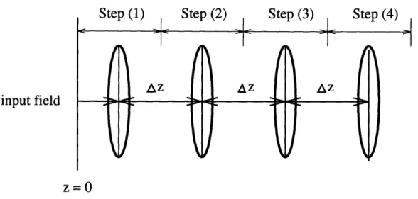
Equation (2.32) can be interpreted as the propagation of the electric wave through a series of equivalent lenses as shown in Figure (2-3).

The first term on the right hand side of (2.32) represents the propagation of the wave through an homogeneous medium with an effective index of n, and length Az/2. The second term of equation (2.32) corresponds to a phase shift associated with propaga-tion through a thin lens and the third term corresponds once again to propagapropaga-tion through an homogeneous medium of length Az/2.

2.4 Solution of the Helmholtz equation for a

Sym-metric Slab Wave Guide

The objective of this section is to find the first fundamental mode of a straight slab wave as shown in figure (2-2). In the case of no change of electric field in the z-direction and y-z-direction and using equation (2.16), equation (2.15) can be simplified to :

-a2 + k2(n 2 - n )0 = 0 _(2.33)

To allow for guided modes in the core : In medium 2 we have na > n2 for Ix J> a

In medium 1 we have nl > na for Ix J< a

(28)

01 = A, cos(k nl - n2x) + B₁ sin(krni - n2x) (2.34)

For the symmetric mode B1 = 0.

Equation (2.33) is solved for the first symmetric mode (TEo) in medium 2 by assuming

2 = A2e-k - + B2ek -x (2.35)

The boundary condition ¢ = 0 when x = 0o gives B₂= 0.

From equation (2.22), the magnetic field in the z-direction is given by :

Hz = 1 (2.36)

3wAo az

Hence the magnetic field in medium 1 is given by :

Hzi = n A sin(k n - nx) (2.37)

and in medium 2 by :

Hz2 = k n - n A2e-k Vn22 (2.38)

jWILo

On the interface between the different media O, and Hz must be continuous. The continuity for ,y gives :

cos(kn -n a)

A2 = A- (2.39)

-kn- 2-n2a

The continuity condition for Hz leads to :

1rni - na tan(kan - n) = _{n - n-} _(2.40)

Equation (2.40) can be rewritten as :

(29)

where:

u = kn - nia (2.42)

w= kina -2 n2a (2.43)

and

v2 = u2 + w2 _(2.44)

It can be shown [13] that for the propagation of a single eigenmode v < i/2 the fiber has mono-mode propagation.

Solving equation (2.40) for nr gives the full solution to the electromagnetic wave equation.

2.5 Solution of the BPM for a curved slab wave

guide

Hocker and Burns (1977) [6] showed that a circular fiber optic can be reduced to a, slab wave guide by using the effective wave guide method. This method replaces a circular wave guide by a slab wave guide by changing the refractive index of the cladding material. The advantage of the effective index method is that it reduces the two-dimensional BPM problem to a one-dimensional problem and hence the number of computations can be reduced by approximately N operations (where N is the num-ber of sample points taken in the one-dimensional case). Typical numnum-ber of step per BPM analysis is 2500 steps (where the step length Az is taken to be equal to 2 pm and the propagation length is 5 mm). Danielson (1984) [2] has reported computa-tional time savings in the order of 100 when the effective index method is used.

Hocker and Burns (1977) [6] also compared the effective-index solution for a two dimensional square waveguide and found that the difference between the effective-index solution and a more rigorous three dimensional solution was a maximum of 10 percent for all values of the cut-off frequency (v). Ramaswamy (1974) [11] found

(30)

similar accuracies to Hocker and Burns (1977) [6] in experimental studies. A fur-ther geometric assumption in the effective index method presented here, is that the power loss in a circular fiber can be approximated by calculating the power loss in a slab waveguide. The validity of the geometric approximation can be deduced from the comparison of slab (without the effective index approximation) and circular step-index guides presented by Love and Winkler (1978) [8] who found that for small radii of curvatures (which dominate power loss in a generally curved waveguide), the slab waveguide give approximately the same results (to within 20 percent) of the circular waveguide. The results presented by Love and Winkler (1978) were also found by Snyder et al (1975) [12]. Preliminary calculations using the step-index method show that for small curvatures, the geometric approximation of the rectangular waveguide to the circular waveguide can give accurate solutions to within 10 percent.

In the case of a slab wave guide, the numerical finite difference evaluation of M in the left hand side of equation (2.19) is :

+ k2 (2.45

Mo = ax2 (2.45)

2nak

M =

p-k

1 +

[

k2(n n )

-

2]

p +

,

+

(2.46)

where m indicates the x position of the finite difference grid, such that x = mAx. In matrix form M can be rewritten as :

Ax2 0 1 22 _{+ k}2_(n?- _n2₎ 1 ₀ AX Ax2 + z a Ax2 0 _Ax1 2 2 + _-ra

...

A0 Ax2 . . . . 1 M=I 2nak 0

(31)

1 0

Ax2

1 2 2 2(

(2.47)

1

The left hand side is seen to be tridiagonal and efficient sparse matrix methods can be used to solve the linear system of equations.

In order to satisfy the curvature paraxiality condition, the curved wave guide can be conformally mapped into an equivalent straight wave guide with refractive index

:[5, 1]

new old (1 + (2.48)

The input electric field at z = 0 is taken to be the first fundamental mode devel-oped in the previous section so that no attenuation occurs due to mode dispersion when propagation occurs through a straight fiber. The input electric field is normal-ized to unity by taking A1 = 1 in equations (2.37) to (2.39).

The BPM analysis for various radii of curvature is performed on a standard mono-mode lossy fiber in order to check whether existing manufactured optic fibers can be used in future sensing applications. The optical characteristics of the fiber are :

* Core diameter : 6pm.

* Core refractive index : 1.4613. * Cladding refractive index : 1.458. * Light wavelength : 1.3pm.

* Propagation step : Az = 2pm. * Propagation distance : 5 mm.

(32)

* Grid spacing : Ax = 0.5p~m.

* Grid length: 128pm.

The refractive index profile and input electric field is given in Figure (2-4).

In order to check the numerical accuracy the of the BPM, fundamental mode propa-gation and power attenuation through a straight fiber is studied. Attenuation losses of -0.009 dB is caused by numerical inaccuracies as a consequence of the finite differ-ence discritization in the x and z directions.

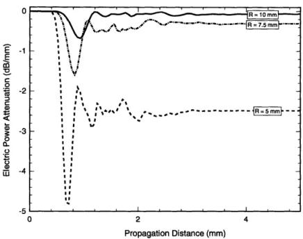
The effect of electromagnetic field propagation along a curve of constant radius is shown in Figure (2-5). The downward movement in peak value of the propagated wave and the carrying of energy in the outer radius cladding shows the typical curva-ture attenuation of the electric field by energy loss through the cladding. Appendix A shows an example calculation of the BPM algorithm for a constant radius curve.

Figure (2-6) shows the power attenuation through curves of various radii. Radii of less than 8 mm show significant power loss while radii greater than 12 mm show insignificant loss. Total power loss is dependent both on radius of curvature and dis-tance of propagation along the curve.

Figure (2-7) shows the rate of power loss with distance occurring in the fibers for various radii of curvature. The large power loss occurring at the beginning of the curve is due to transition losses. During the transition porition of the propagation, the input straight slab fundamental mode changes to the curved waveguide funda-mental mode as shown in Figure (2-5). Transition loss occurs due to the dispersion of energy within the transition length as the input fundamental mode changes to the curved fundumental mode.

(33)

loss. Marcuse (1971) [9] obtained an approximate closed form solution for the steady state bend loss of constant curvature wave guides given by :

2w3 R +wa

WU2e n2k2-u 2

a = 4.34 in dB/unit length (2.49)

v2 nik 2 2

()

The comparison of the theoretical solution and numerical solution is shown in Figure

(2-8).

The relative contribution to total power loss of the steady state propagation and transition loss in an arbitrarily curved wave guide is dependent on :

* Propagation distance - steady state propagation loss dominant. * Radius of curvature - both losses dominant.

* Changes in curvature - transition loss dominant.

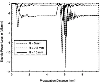
For small distance propagation along a curvature changing fiber, the transition loss is dominant. This effect can be studied by calculating the curvature loss in a constant radius "S" curve. An "S" curve has the characteristics of having two transition losses. The rate of attenuation with distance in a "S" curve is shown in Figure (2-9). The large transition losses occur near propagation distances of 0 and 5 mm corresponding to the position of abrupt curvature change.

The abrupt decrease in attenuation loss at propagation distances of 5 mm (just be-fore the large transition losses) shown in Figure (2-9) corresponds to break down in the BPM paraxial assumption. The abrupt change in curvature at this distance re-quires the propagating fundamental electric field to change abruptly which violates the paraxial assumption. Since the constant bend radius loss is re-established after approximately 8 mm, it can be noted that after the break down in paraxial assump-tions which occur over a short distance (between approximately 5 and 5.5 mm) the field eventually behaves consistently with the paraxial assumptions. It must be noted that the BPM results give no indication whether the transition losses after the abrupt

(34)

curvature change are accurately calculated. It can be concluded that the break down in paraxial assumptions lead to small inaccuracies with respect to total power losses provided that the BPM assumptions are not violated frequently and thus make up only a small percentage of the total power loss.

2.6 Wave Guides used for Sensing

It is suggested here that fiber optic sensors relying on detection of host material dam-age by curvature change, should be step-indexed mono-mode cylindrical fibers. This type of fiber has the advantage of being more sensitive to curvature loss than other fibers since slight deviations from straight transmission causes electromagnetic loss into the cladding and the fiber. In sensing applications where the inclusion of the sensing element causes strength loss in the host material (such as in strain sensing of composites), the mono-mode fiber has the added advantages of having a smaller diameter.

The success of the fiber optic sensor is dependent both on the sensitivity of the sensing and detection device. Though the production cost of fibers are essentially independent of sensitivity, the cost of detection equipment is strongly dependent on sensitivity. Expensive detection equipment is capable of detecting losses in the 0.01 dB range while relatively inexpensive detection equipment operates in the 5 dB sens-ing range. Hence, it is advisable to design the fiber with optimal sensitivity so as to reduce the detection equipment cost and at the same time avoid excessive power loss at each crack (otherwise onlt a small number of cracks can be detected with each fiber).

For desirable fiber sensor design, a theoretical model relating crack opening to the optimal power loss needs to be developed. This is the focus of the next 3 chapters of the present thesis.

(35)

Bibliography

[1] R. Baets and P.E. Lagasse. Loss calculations and design of arbitrary curved

integrated-optic waveguides. J. Opt. Soc. Am. 73. 177-182 (1983)

[2] P. Danielson. Two-dimensional propagating beam analysis of an electrooptic

waveguide modulator. IEEE J. Quantum Electron. 20. 1093-1097 (1984)

[3] M. D. Feit and J. A. Fleck. Computation of mode properties in optical fiber

waveguides by a propagating beam method. Appl. Opt. 19. 1154-1164 (1980)

[4] J. A. Fleck, J. R. Morris and M. D. Feit. Time dependent propagation of high

energy laser beams through the the atmosphere. Appl. Phys. 10 129-160 (1976).

[5] M. Heiblum and J. Harris. Analysis of curved optic waveguides by conformal

transformation. IEEE J. Quantum Electron. 11. 75-83 (1975)

[6] G. B. Hocker and W.K. Burns. Mode dispersion in diffused channel waveguides

by the effective index method. Appl. Opt. 16. 113-118 (1977)

[7] R.M. Knox and P.P. Toulios. Integrated circuits for the millimeter through

opti-cal frequency range. Proceedings of M.R.I. Symposium on Submillimeter Waves.

J.Fox ed. (Polytechnic,Brooklyn). 99-107 (1970)

[8] J.D. Love and C. Winkler. Power attenuation in bent multimode step-index slab

and fibre waveguides. Electron. Lett. 14. 32-34. (1978)

[9] D. Marcuse. Bending Loss of the assymetric slab waveguide. Bell Sys. Tech. J.

(36)

[10] W.H. Press et al. Numerical recipes in FORTRAN: the art of scientific

comput-ing. (Cambridge University Press, Cambridge). (1992)

[11] V. Ramaswamy. Strip Loaded Film Waveguide. Bell Sys. Tech. J. 53. 697-704 (1974)

[12] A.W. Snyder, I. White and D.J. Mitchell. Radiation from bent optical wavegiudes. Electron. Lett. 11. 332-333. (1975)

[13] W. van Etten. Fundamentals of Optical Fiber Communication. (Prentice Hall, New York). (1991)

[14] C. Vassallo. Reformulation of the beam-propagation method. J. Opt. Soc. Am. A 10. 2208-2216 (1993)

[15] R.G. Walker. The design of ring resonators for integrated optics using silver

ion-exchange waveguide. Ph.D. dissertation (Glasgow University, Glasgow). (1981)

[16] D. Yevick and B. Hermansson. New formulation of the matrix beam propagation

(37)

ouput light field

Figure 2-1: Geometric propagation of EM waves along a curved optic wave guide.

a---a

(38)

input field

5Ctnn (((

z=0

Figure 2-3: An array of lenses equivalent to the beam propagation expressed in Equa-tion (2.32). 0.0 -60 -40 -20 0 20 40 60 1.4620 1.4610 1.4600 1.4590 .* 1.4580 1.4570 1 4560R x (lm)

Figure 2-4: Refractive index profile and normalized input electric field for a mono-mode step index slab wave guide.

(39)

0.4

0.2

0n

-60 -40 -20

Figure 2-5: Electric field attenuation at wave guide. Radius of curvature is 8 mm.

Co

S

_c) o 0 L aw 0 0e₀ 0 20 40 60 x (gpm)

discrete distances for a constant curvature

4 6 8 10 12 14

Radius of Curvature (mm)

Figure 2-6: Electric field

gation length = 5 mm

(40)

Propa-Propagation Distance (mm)

Figure 2-7: Rate of power attenuation for various constant radii of curvature.

5 7 9 11

Radius of Curvature (mm)

Figure 2-8: Comparison of theoretical solution obtained by Marcuse and BPM results.

' - ' - 'lR = 10 mm . S • --- I _I?I I _i. M !? i ill ! i rl -I I I I III5; t b• i I I 1 I I I I I I S III S II I I I I - I II II S IIII_II

(41)

-2 E -4 0 _tr-6 -8 o o. o -10 U -12 -4 ii - i " ... -J . i I il --- R=7.5mm = 10mI i-i . _iI. i r. 1 1 1 1 1 . 1 1 1 1 1 1 . I l~~ r r I l l s I 0 2 4 6 8 Propagation Distance (mm)

Figure 2-9: Rate of power attenuation through S - curve of various radii.

(42)

Chapter 3 Mechanical Behaviour of an Optic

Fiber Under Bending

3.1 Introduction

Chapter 2 has shown that electric field attenuation in an optic waveguide is strongly dependent on the axial curvature distribution of the fiber. This section deals with the numerical modelling of the mechanical behaviour of an optic fiber sensor in a matrix material.

The mechanical behaviour of reinforcing fibers in cracked matrix material have been investigated by several authors. The mechanical model proposed by Leung [1] ana-lyzed the behaviour of a steel fiber embedded in an elastic matrix by assuming that the continuum interaction of a fiber bearing on the matrix could be modelled as a beam on an elastic foundation. Stang and Shah [3] proposed a theoretical model of a fiber subjected to pullout with debonding. Previous models have the problems of either assuming the fiber to act in plane strain or subject to pure Mode I crack opening. The model proposed in this section is an extension of Leung [1] beam on elastic foundation model with the equivalent matrix stiffness being calculated by a three dimensional finite element analysis. The effect on the equivalent foundation stiffness of a soft bedding layer such as a fiber jacket is also included in this section.

(43)

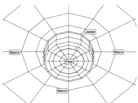
3.2 Physical Model of Fiber Matrix Interaction

A crack occurring in a material can propagate under three modes (labelled I, II and III). The analysis presented herein only considers the in-plane propagation modes (I and II) caused by tension and shear action in one plane. General out of plane crack propagation is ignored in the analysis since electromagnetic tools for analysing generally curved three dimensional waveguides have not yet been developed and it is unlikely that the paraxial assumption of mode propagation used in the BPM is valid.

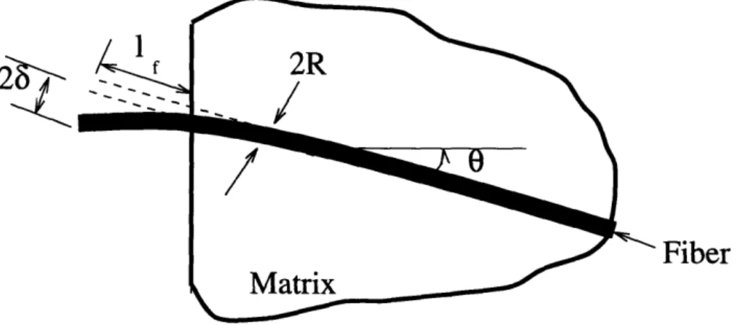
Only analysing in-plane crack propagation means that the assumed physical model is as shown in Figure (3-1). Figure (2.1) shows a generally oriented fiber in the crack plane, bridging an opening crack. Due to the orientation of the fiber to the crack face, far field applied tension will cause coupled shear, bending and extension in the fiber. This work focuses on Mode I (tension) crack propogation, though the work can readily be extended to Mode II (shear) crack action by varying the prescribed displacements on the fiber.

Morton and Groves [2] have shown that for a fiber crossing the crack faces, the phys-ical model shown in Figure (3-1) above can be reduced to the one shown in Figure (3-2). The assumption in Figure (3-2) is that the fiber is located at such a distance from the crack tip that the rigid body crack face movements can be considered par-allel. This assumption allows for the modelling of half the fiber and corresponding matrix due to symmetry.

Figure (3-2) shows the geometric changes in the fiber undergoing a crack opening, u has two components given by :

6 = u sin 0 (3.1)

(44)

The dimensions of a standard mono-mode optic fiber typically used for fiber optic sensing are :

* Fiber radius : R = 62.5 pm.

* Fiber jacket thickness : t = 37.5 pm

3.3 The Finite Element Model

The physical model given in Section (3.2) above can be further simplified by assuming a fixed far boundary at a distance of 5 fiber diameters from the fiber center which by Saint Venant's principle should allow for complete stress homogenization mean-ing that there is no variation in stresses along the far boundary. Figure (3-3) shows the mathematical model derived from the physical model with the far boundary as-sumption. The materials in the model are assumed isotropic and linearly elastic with material constants :

* Glass fiber : Young's Modulus 70 GPa. Poisson Ratio 0.2. * Plastic jacket : Young's Modulus 3 GPa. Poisson Ratio 0.2. * Cement Matrix : Young's Modulus 20 GPa. Poisson Ratio 0.2. The assumptions behind the Finite Element Scheme are :

Separation between fiber and matrix on the tension zone is allowed for by leav-ing a thin zone free of elements at the fiber-matrix interface. The length of the separated zone is taken to be one fiber diameter which approximately cor-responds to the length of the tensile zone. It must be noted that the effect of various assumed material properties in the separated zone (E varying from zero for complete fiber-matrix separation to E equal to matrix stiffness for no seperation) only effects the center line deflection by approximately 5% which is considered to be adequately accurate for this analysis.

(45)

* Loading corresponding to the prescribed deflections are governed by Mode I and Mode II crack movements.

Eight node linear brick elements with various meshing schemes were used to compare mesh sensitivity. The mesh shown in Figure (3-4) was chosen since it was found to optimize both accuracy and computational time. The final finite element model has the following characteristics.

* Number of elements 2460. * Number of nodes 2736.

* Radial far boundary at 5 fiber diameters. * Axial far boundary at 12 fiber diameters.

3.4 Finite Element Results

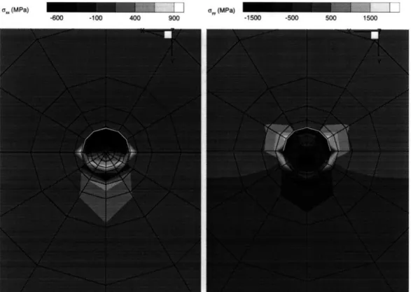
The effects of varying fiber-matrix incidence angle and crack opening displacement is presented elsewhere. The results of simulations on a fiber with incidence angle of 30' with crack opening of 0.2pm is presented in this section in order to clarify some key features in the finite element model for a typical fiber orientation and crack opening displacement.

The band plots presented in Figures (3-5 a) and (3-5 b) show the in-plane stress distributions at a distance of one fiber diameter from the crack face for a fiber with a soft jacket coating. Figures (3-6 a) and 3-6(b) show the in-plane stress plots for a fiber with no jacketing material. Comparing Figures (3-5) and (3-6) shows that for the jacketed fiber, the jacket material carries most of the stresses and only relatively small stresses are transferred to the matrix. The stresses at the far boundary are found to be homogeneous thus validating the far boundary assumption.

(46)

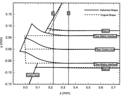
line, the fiber outer radius and jacket-matrix boundary. The relatively small differ-ence in deflected shape between the fiber center line and fiber outer radius implies that the fiber center-line remains almost parallel to the outer radius. The relatively large difference in deflection between the fiber center line and jacket interface implies that most of the deflection occurs within the jacket and hence most stress transferal occurs within the jacket region. The difference in deflected shapes of the fiber and jacket can be seen by comparing the deflections at the crack face and along the line marked A. The matrix-jacket interface has essentially zero deflection past the crack face while the glass fiber has deflections past line A. The fiber enters the matrix at the crack face, thus the deflections of the jacket to the left of the crack face are due to the free applied fiber deflections, while deflection to the right of the crack face include the effect to matrix jacket interaction. Figure (3-8) shows the deflected shape of the fiber with no jacketing material. Notice that there are substantial deflections in the matrix past the crack faces. Hence it can be concluded that the presence of a jacket help to reduce the deflections (and the stresses) in the matrix.

Figures (3-5) and (3-7) show that most stress transferal occurs within the jacket. Figures (3-9) show the in-plane stress distribution at two fiber diameters from the crack face in a jacketed fiber. Comparing Figures (3-9) and (3-5) it can be seen that the stresses in the matrix at a distance of two fiber diameters is substantially less than the stresses at one fiber diameter. Spalling of the matrix is associated with micro-cracks and defects occurring within the material. Due to the rapid decay of stresses in the matrix and the associated small stresses transferral from fiber to matrix, it is unlikely that the matrix will spall or crush and the linear elastic assumption for the matrix behaviour is valid.

The apparently anamolous phenomena of tensile stresses (ay,) above the debonded zone in Figure (3-9) are due to the large tensile stresses associated with the end of the debonded zone. Figure (3-10) shows the relatively large (aY,) stresses at the end of the debonded zone. Similarly zones of stress concentrations occur in the x-y plane where the debonded zone ends as shown in Figures (3-5). By filling the debonded

(47)

gap with low stiffness material it was found that the magnitude of the stress concen-trations could be reduced, and the effect of the material had no significant effect on changing the deflected shape of the fiber center-line.

Figure (3-11) shows the small radius of curvature in the fiber associated with the 0.2 mm crack opening.

3.5 Beam on Elastic Foundation Analysis of Fiber

Behaviour

Leung [1] showed that the action of an embedded fiber in a matrix material subjected to bending deflection can be modelled as a beam on an elastic foundation provided that the shear stiffness of the matrix material is much smaller than the in-plane stiff-ness of the fiber.

The equivalent stiffness of the three dimensional behaviour is studied in the following way.

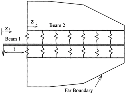
Consider an elastic beam on a soft founding material as shown in Figure (3-12).

The response of this beam can be analyzed by solving the following differential equa-tions : For Beam 1 : d4yl_d4_Y ₌₀ _(3.3)

dz1

For Beam 2: d4y2 dzY = 4044y2 (3.4) where:

(48)

z is the distance along the beam.

8 is the relative stiffness term = k/EI. k is the stiffness of the foundation.

E is the Modulus of Elasticity of the beam. I is the Moment of Inertia.

The boundary conditions are :

y₁= u at z₁= 0.

y, = 0 at zl = 0 (Zero Moment Condition).

The kinematic and static equivalence at the beam-matrix connection gives :

Y1 = Y2 at 1 = l vy' = y at zl=l

Y1 = Y2 at z =l

Y1 = Y2 at z1= 1

The zero deflection and slope conditions at the far boundary gives :

Y2 = 0 _at _Z

2 = 00

y =O0 at z2 = 00

(3.11) (3.12) Here a prime denotes a differentiation with respect to axial distance z.

The solution of this differential equation is :

For z1 < 1 :

(3.5)

(3.6)

(3.7)

(3.8)

(3.9) (3.10)

(49)

z3/3 - 3zfP(1 2_/32 ₊_21±_{+ 1)}

213/3 +612P2+610+3

For Z₂> 0

3e(-z2) [(1• + 1)cos(zil) - l/sin(/zi)] (314)

2133 + 612/2 + 610 + 3

The schematic representation in Figure (3-13) shows that in general the stiffness of the equivalent foundation can be taken as a monotonically increasing function with length of fiber embedded in the matrix. This is due to the fact that at the crack face, the bearing matrix area is negligible.

The generalized differential equation for a straight fiber with arbitrary founding stiff-ness properties can be expressed by :

d4y

dz4 4_(z)y _(3.15)

dz4

It must be noted that equation (3.15) is still linear even though the relative stiffness term 0 is any function of z.

In this case the variation in stiffness is assumed linear and the governing equation becomes:

dz4

dz4

__

4zy

(3.16)

The boundary conditions are the same as in equations (3.5) to (3.12).

The standard method of solution of this type of non-homogeneous differential equa-tion is by substituting y = Eaizi. The substitution gives the following solution :

Damage detection in civil and aerospace structures with fiber optic sensors

Damage Detection in Civil and Aerospace Structures with.

Fiber Optic Sensors

Niell Glen Elvin

. ...

...

OCT

25 1995

Damage Detection in Civil and Aerospace Structures with

Fiber Optic Sensors

by

Niell Glen Elvin

Abstract

Acknowledgments

Contents

List of Figures

Equation (2.32

).

. . . .

. . . .. .

38

Notation

-

Electromagnetic analysis

Notation - Mechanical analysis

Notation

-

Delamination Analysis

Chapter 1

Introduction

Chapter

Electromagnetic Wave

Propagation

2.1

Optical Wave guide Basics

2.1.1

Basic Electromagnetic Definitions

(2.1)

(2.2)

(2.3)

c =

(2.5)

2.1.2

Wave Guide Definition

2.1.3

Wave Guide Characterization

2.2

Analysis of EM Transmission in a Slab Wave

Guide

aB

OH

V x E =--=

o

(2.8)

at

at

aD

at

at

OE

a

at

W atd

(2.13)

(2.15)

2.3

Solution of the Helmholtz Equation by the

Beam Propagation Method

I(x,

y,

z)

=

/(x,

y,

z)e

(2.16)

ao

2.3.1

Formulation of the Beam Propagation Method

2.3.2

_(2.16)

_{- k}